Integrating Transformer and GCN for COVID-19 Forecasting

Abstract

The spread of corona virus disease 2019 (COVID-19) has coincided with the rise of Transformer and graph neural networks, leading several studies to propose using them to better predict the evolution of a pandemic. The inconveniences of infectious diseases make it important to predict their spread. However, the single deep learning (DL) model has the problems of unstable prediction effect and poor convergence. When calculating the relationship between different positions within a sequence, Transformer does not consider the local context in which each position is located, which can make the prediction vulnerable to outliers, so the integration of the graph convolutional network (GCN) to capture local information is considered. In this paper, we use Transformer to encode the time sequence information of COVID-19 and GCN to decode the time sequence information with graph structure, so that Transformer and GCN are perfectly combined and spatial information is used to further study the integration of these two methods. In addition, we improve the traditional positional encoding structure and propose a dynamic positional encoding technique to extract dynamic temporal information effectively, which is proved to be the key to capture spatial and temporal patterns in data. To make our predictions more useful, we only focused on three states in the United States, covering one of the most affected states, one of the least affected states, and one intermediate state. We used mean absolute percentage error and mean square error as evaluation indexes. Experimental results show that the proposed time series model has better predictive performance than the current DL models. Moreover, the convergence of our model is also better than the current DL models, providing a more accurate reference for the prevention of epidemics.

1. Introduction

The Corona Virus Disease 2019 (COVID-19) epidemic struck the globe at the start of 2020, with death tolls rising all around the globe. Different regions experienced differing degrees of economic, social, and political disruption as a result of the public health emergency [1]. To reduce the epidemic’s negative impact, contain the virus source’s spread before the epidemic develops, evacuate and control the surrounding people who may be exposed to the virus source, and prevent a second outbreak of the epidemic, act quickly to contain the virus source’s spread before the epidemic develops [2]. For the time being, this exposes the world to a serious public health issue that we must address in terms of controlling developing infectious illnesses. Understanding future trends is also a key aspect of preparedness measures as the number of confirmed COVID-19 cases continues to rise [3]. Because the epidemic has not been adequately managed in some countries, forecasting COVID-19 developments has been a prominent research topic. With the shift and evolution of COVID-19 around the world, effective models have been proposed and successfully used to epidemic prevention and control techniques in some locations, which is critical to the COVID-19 pandemic’s suppression. Simultaneously, the regularly employed assessment indicators and representative trend prediction models in this sector have significant relevance as a reference for future epidemic management [4].

The conventional epidemic prediction model is currently the most common traditional trend forecast tool. However, the traditional infectious illness trend forecast method does not take into account the current state of infectious disease preventive and control methods, and the model is not ideal. While COVID-19 is extensively contagious, and the route of transmission of COVID-19 may be determined using different infection instances in all other infectious diseases, the SIR model is the most classical model in the prediction of infectious disease models. However, compared with the traditional SIR model, due to the particularity of COVID-19, such as there being no closed case, an open system is considered; patients will be isolated immediately after diagnosis, so as not to be a new source of infection [5,6]. The SIR model needs to be appropriately modified to consider more factors, and then parameters of the model can be obtained through real-time data fitting, so as to achieve the effect of predicting epidemic trend changes at different stages. Traditional methods rely on a large amount of expert experience and knowledge, and it is difficult to make accurate prediction for dynamic factors and timing information in complex environments. With the increasing data scale, it is difficult for existing models to make accurate prediction [7,8].

With the advent of Deep Learning (DL), researchers at home and abroad have built COVID-19 trend prediction models based on DL. These models have effectively assisted medical experts and scientific research institutions to efficiently predict COVID-19. Many scholars use the theory of DL to build models to analyze different situations and predict the development trend of the epidemic [9,10]. DL is a deep nonlinear network composed of multiple hidden layers that allows machine systems to learn to analyze like humans by abstracting features into more abstract features or higher categories [11]. In recent years, it has made unprecedented achievements in classification, detection, recognition, prediction and other tasks, and has attracted wide attention from all walks of life. In the process of DL, we can solve the problems that are difficult to be solved by traditional machine learning such as high dimension and complexity in massive data [12,13]. Therefore, in the context of the outbreak of the global epidemic crisis, DL is widely used to help us quickly and accurately predict the probability of critical illness of COVID-19 patients, carry out dynamic monitoring of the epidemic and predict the future development trend of the epidemic. The key reason for the good effect of DL in prediction is that artificial neural networks imitate human brain to do similar work by connecting weight structure and activation function, and its application in the prediction of infectious diseases is more and more extensive [14].

Specifically, Transformer architecture and graph convolution network (GCN) have achieved good results in the field of DL. The encoder encodes the input data, which is then decoded by the decoder network to produce the desired output based on the encoded input. Because these networks have a better understanding of context, they provide better performance. However, the overall performance of the model in the prediction problem still has a lot of room for improvement, and the way of encoding and decoding still needs to be improved [15,16].

Transformer does not take into account the local environment of each location when calculating the relationships between different locations within a sequence, which can make predictions susceptible to outliers. Therefore, we propose a hybrid encoder-decoder architecture, which encodes the timing information through the Transformer and decodes the feature engineering vector with timing information through the GCN, so as to obtain the accurate prediction of COVID-19 diagnosis rate and mortality. Secondly, we improve the traditional position encoding technology and propose a Dynamic Positional Encoding (DPE) technology to effectively extract the dynamic timing information and enhance the performance of neural network. The experimental results show that the prediction performance and the convergence of the proposed model is better than the existing DL models and provides an effective model for complex time series prediction.

This paper is structured as follows. Section 2 reviews the prediction model of COVID-19 development trend based on DL. Section 3 describes the data characteristics and data sources. Section 4describes data preprocessing, COVID-19 model, training data, and prediction accuracy measurement. The performance of the model is compared and analyzed. Experimental results are given in Section 5. Section 6 concludes this paper.

2. Literature Reviews

There are various prediction approaches for sexually transmitted diseases in the field of DL, which may be split into qualitative and quantitative prediction based on the hypotheses of each method. Some methods, of course, combine the two processes for a more thorough prediction. Rahimi et al. [17] reviewed and briefly analyzed the most important machine learning prediction models for COVID-19.

When analyzing the influence of imported cases on national epidemic prevention and control, Kim et al. [18] proposed that the number of imported cases in a country is directly proportionate to the number of inbound passengers and confirmed cases in the country. This complicated spatio-temporal link is incorporated into the COVID-19 predictive model, which successfully uses the power of a deep neural network to assess the influx of COVID-19 cases from abroad, based on epidemic trends and the risk of infection abroad. Restrictive policies can harm the economy, but a flexible attitude can put a big portion of the population at danger. Miralles-pechuan et al. [19] developed the SEIR epidemiological model and used a combination of deep Q learning and a genetic algorithm to forecast COVID-19 viral evolution in the community. The survey by Shorten et al. [20] looks into how DL might help tackle the COVID-19 pandemic and offers recommendations for future research. The current state of DL is assessed first, followed by a summary of the major constraints of DL in the implementation of COVID-19. In the above work, COVID-19 was mainly predicted by using a DL model combined with a traditional model. The prediction accuracy was improved to some extent, but the generalization performance of the model was not improved and the optimization performance under different data sets could not be guaranteed. Therefore, this paper considers the DL approach and discards the use of traditional models.

Farsani et al. [21] suggested a new time series prediction approach that can generate more accurate predictions in a longer interval than previous methods. The Transformer neural network based on self-attention is very good at predicting time series problems, and the model’s performance is equivalent to that of other tools. Based on static and dynamic site features, La et al. [22] introduced a new machine learn-based framework capable of predicting parameters of any epidemiological model, such as exposure and recovery rates. A spectral temporal graph neural network was proposed by Cao et al. [23] (StemGNN). In the spectral domain, StemGNN captures intersequence and temporal correlation. The spectrum representation displays unambiguous patterns after passing through graphical Fourier transform and discrete Fourier transform, which may be efficiently predicted by convolution and sequence learning modules. Advanced neural networks, such as Transformer and graph neural networks, were mainly used in the above work to predict epidemics. However, previous work has not fully considered the merits of different advanced models. Therefore, this paper integrates the advantages of efficient DL prediction models to further accurately predict key indicators such as the number of infections, deaths, and vaccinations for COVID-19 by designing a network architecture for a hybrid prediction model.

3. Data Reduction

To make our predictions more meaningful, we just focused on three states of the United States (US) that is to cover two of the highest affected states, the lowest affected states, and one intermediate state. The three states are New York (NY), Virginia (VA), and California (CA). We have focused mainly on the forecasting of the number of confirmed cases, deaths, and vaccines. Two datasets are considered for our work. The first is cases and deaths and the second is vaccines.

3.1. Confirmed Cased and Deaths Datasets

We use a dataset from the New York Times [24]. This is a 16-month data series that is updated daily and spans the months of January 2020 to 5 May 2021. Additionally, since 22 April 2021, the index stands at around 418 data points. This dataset contains information related to the following the US:

• Date: Observation date in mm/dd/yyyy
• State: State of the USA
• Cases: Cumulative counts of coronavirus cases till that date
• Deaths: Cumulative counts of coronavirus deaths till that date

In

Table 1. The structure of the cases and deaths dataset.

Date	State	Cases	Deaths
22 April 2021	Texas	2,868,207	49,984
22 April 2021	Utah	394,398	2178
22 April 2021	Vermont	22,325	243
22 April 2021	Virgin Islands	3068	27
22 April 2021	Virginia	650,981	10,653
22 April 2021	Washington	393,514	5472
22 April 2021	West Virginia	150,288	2808
22 April 2021	Wisconsin	654,681	7438
22 April 2021	Wyoming	57,613	705

, we can see an example of the dataset. There is a similar dataset [25], but it is only updated until February 2021 and is not continuously updated. We chose this option because of this. After conversion to sliding window blocks, the New York Times maintains this dataset. In an 80:20 ratio, we divide the dataset into two parts: training and testing. The first 80% of the data is used for training, while the remaining 20% is used for evaluation.

3.2. Vaccinations Dataset

We use the dataset provided by our world in data [26] as state level data vaccination. This time series data starts on 13 January 2021 and runs until 5 May 2021. It is updated daily and contains the following features:

• Date
• State Name
• Daily count of vaccinations

This dataset is quite small, as it only contains three months’ worth of data. We decide to reduce the size of the slider window to increase the number of samples and split the dataset into 80:20 training and test datasets to ensure that we had enough days to evaluate it.

4. Architecture Design for Hybrid Models

4.1. Data Preprocessing

To begin, data for COVID-19 are obtained from an open-source dataset. Second, we perform data pre-processing operations on the number of infections data, such as outlier processing and null processing, to obtain standard time-series data. The sample data are taken from the first month of a single data sample, and the remaining data are used as the label data. Finally, these data samples are fed into a training model that can predict data for the remaining time behind based on the first 80% of the data for the purpose of predicting future data based on the first 80% of the data. Figure 1 depicts a global visualization of the number of confirmed cases in the US.

4.2. Model Theory

In this paper, we propose a hybrid model based on the Transformer [27] and GCN [28], creativity will be a combination of these, and put forward a kind of DPE structure, efficient trap decoding topological structure of the information and the potential relationship between point and point, promote the overall performance of the model. The framework of our model to deal with COVID-19 is shown in Figure 2, where the encoder takes the time series data as input and the decoder part predicts the future values in an autoregressive manner. The decoder is connected to the encoder using Multi Head attention (MHA). In this way, the decoder learns to “focus” on the most useful parts of the time series history before making predictions, and the decoder uses the convolution operation of GCN to capture local information and improve the overall prediction of the model. The following article introduces related concepts and basic knowledge.

4.2.1. Encoder Structure

$DPE$ can encode the embedding of the initial starting information in a cyclic and dynamic manner, overcoming the classic position coding operation’s limitation of only being applicable to linear sequences and effectively retrieving the position information of dynamic nodes. Here, $DPE$ is defined as [29]:

$$DP{E}_{t,i}=\{\begin{array}{l}\sin \left(2\pi f_{i}t+\frac{2\pi }{{\omega }_{d}i}\right),\begin{array}{ccc}i& is& odd\end{array}\\ \cos \left(2\pi f_{i}t+\frac{2\pi }{{\omega }_{d}i}\right),\begin{array}{ccc}i& is& even\end{array}\end{array}$$

(1)

where

$$f_i=\frac{{10000}^{\frac{d}{2i}}}{2\pi }$$

(2)

$${\omega }_d=\{\begin{array}{cc}\frac{3\left[d/3\right]+1}{d}\left(N-N^{\frac{1}{\left[d/2\right]}}\right)+\frac{1}{\left[d/2\right]},& \begin{array}{cc}if& d<\left[\frac{d}{2}\right]\end{array}\\ N& ,otherwise\end{array}$$

(3)

$DP{E}_{t,i}\in R^d$, $t$ is the location of node and $d=128$ is the embedding dimension, $i\in \left\{1,2,\dots ,n\right\}$, the angular frequency ${\omega }_d$ is decreasing along the dimension to make the wavelength longer within the range $N$.

After the initial information is processed by the $DPE$ layer, the incoming graph is embedded into the network layer ($n$ = 3, updated three times). For each network layer, there are two sub-layers: MHA and Feed Forward (FF). Similar to literature [27], $MHA$ is used to extract node information of different types. Sub-layers $l\in \{1,\dots N\}$ and $h_i^l$ are defined as point embedding of each node, and the output $\{h_0^{(l-1)},\dots ,h_n^{(l-1)}\}$ of $l-1$ layer is the input of $l$ layer. MHA of each layer can be expressed as follows:

$$q_{im}^l=W_m^Q{h}_i^{l-1},k_{im}^l=W_m^K{h}_i^{l-1},v_{im}^l=W_m^V{h}_i^{l-1}$$

(4)

$$u_{ijm}^l={(q_{im}^l+DP{E}_{im})}^T{k}_{jm}^l$$

(5)

$$a_{ijm}^l=e^{u_{ijm}^l}/{\displaystyle {\sum }_{j=0}^n{u}_{ijm}^l}$$

(6)

$${h^{\prime }}_{im}^l={\displaystyle \sum _{j=0}^n{a}_{ijm}^l{v}_{jm}^l}$$

(7)

$$MH{A}_i^l(h_0^l,\dots ,h_n^l)={\displaystyle \sum _{m=1}^M{W}_m^O}{h^{\prime }}_{im}^l$$

(8)

where the head of attention $M=8$, $m\in \{1,\dots ,M\}$, query vector $q_{im}^l\in R^{d_k}$, key vector $k_{im}^l\in R^{d_k}$ and value vector $v_{im}^l\in R^{d_v}$ are calculated by trainable parameters $W_m^Q\in R^{d_k\times d_h}$, $W_m^K\in R^{d_k\times d_h}$ and $W_m^V\in R^{d_v\times d_h}$ respectively. The final vector is evaluated by $W_m^O\in R^{d_h\times d_v}$ ($d_k=d_v=d_h/M=16$).

After MHA processing, deep node information is captured, with vector $h_i^l$ passing in Batch Normalization (BN) [30] and FF layer [31], where each node $i$ is calculated as follows:

$${\widehat{h}}_i^l=\tanh (h_i^l+MH{A}_i^l(h_0^{l-1},\dots ,h_n^{l-1}))$$

(9)

$$FF({\widehat{h}}_i^l)=W_1^F\mathrm{Re}Lu(W_0^F{\widehat{h}}_i^l+b_0^F)+b_1^F$$

(10)

$$h_i^l=\tanh ({\widehat{h}}_i^l+FF({\widehat{h}}_i^l))$$

(11)

where $h_i^l$ is computed by the trainable parameter $W_0^F\in R^{d_F\times d_h}$, $W_1^F\in R^{d_F\times d_h}$, $b_0^F\in R^{d_F}$, $b_1^F\in R^{d_h}(d_F=4\times d_h)$.

4.2.2. Decoder Structure

Let $x_i^l$ indicate the feature vector at layer $l$ associated with node $i$ in the GCN network ConvNet. Applying a non-linear transformation to the feature vectors $x_j^l$ for all nodes $j$ in the neighborhood node $i$ yields the activation $x_i^{l+1}$ at the following layer. Thus, the most generic version of a feature vector $x_i^{l+1}$ at vertex $i$ in a graph ConvNet is [28]:

$$x_i^{l+1}=f(x_i^l,\{x_i^l:j~i\})$$

(12)

where $\{j~i\}$ denotes the set of neighboring nodes centered at node $i$. In other words, a graph ConvNet is defined by a mapping f taking as input a vector $x_i^l$ as well as an un-ordered set of vectors $\left\{x_j^l\right\}$. The arbitrary choice of the mapping f defines an instantiation of a class of graph neural networks such as [32].

In this work, we leverage the graph ConvNet architecture introduced in [28] by defining node features $x_i^{l+1}$ and edge features $e_{ij}^{l+1}$ as follows:

$$x_i^{l+1}=x_i^l+\mathrm{Re}LU(BN(W_1^l{x}_i^l+{\displaystyle \sum _{j~i}{\eta }_{ij}^l}\odot W_2^l{x}_j^l)) with {\eta }_{ij}^l=\frac{\sigma (e_{ij}^l)}{{\displaystyle {\sum }_{j^{\prime }~i}\sigma (e_{i{j}^{\prime }}^l)+\epsilon }}$$

(13)

$$e_{ij}^{l+1}=e_{ij}^l+\mathrm{Re}LU(BN(W_3^l{e}_{ij}^l+W_4^l{x}_i^l+W_5^l{x}_i^l))$$

(14)

where $W\in R^{h\times h}$, $\sigma$ is the sigmoid function, $\epsilon$ is a small value, $\mathrm{Re}LU$ is the rectified linear unit, and $BN$ stands for batch normalization. At the input layer, we have $x_i^{l=0}={\alpha }_i$ and $e_{ij}^{l=0}={\beta }_{ij}$.

4.3. Training Schemes

Based on the Pytorch-1. 7. 0 deep learning platform, a single Nvidia RTX 1650 GPU was used to run our model and the compared DL models on Windows 10 OS. The original COVID-19 data are separated into two sets in 8:2 ratio: a training set and a test set. The validation set is generally used to identify the model’s network structure and change the hyperparameters. The training set is mostly used to train the model and decide the weight model, and the validation set is primarily used to assess the model’s generalization capacity. The head of the MHA in encoding $H$ = 8, the dimensionality of both the $FF$ input and output layers is 512 dimensions, and the GCN decoding of the implicit layer vector using $l=3$. The learning rate of the Adam optimizer is $\eta ={10}^{-3}$ and the decay rate of the weights is $w={10}^{-6}$. We provide the optimization metrics Mean Absolute Percentage Error (MAPE) and Mean Square Error (MSE) of the model on the three COVID-19 datasets in our experiments, and also provide comparative plots of the convergence and fit of the model.

4.4. Prediction Accuracy Measurement

MSE, root mean square error, mean absolute error, and MAPE are four commonly used indicators in regression prediction tasks. The square of the difference between the estimated and true value of a parameter is referred to as MSE. MSE can determine how much data has changed. Because finding the derivative by square is simple, it is frequently used as the loss function in linear regression. The MSE value is a measure of how well a prediction model can describe experimental data.

MAPE is calculated by summing the normalized absolute differences between actual and anticipated values and dividing them by total values. Because of its extremely obvious interpretation in terms of relative error, MAPE is also employed as a loss function for regression issues and model evaluation. The smaller the MAPE, the better the model. Its value is shown to be between 0 and 1, with 0 MAPE being the optimal model. MSE is calculated by summing the squared differences between actual and anticipated values and dividing by total values. Therefore, MSE and MAPE are used as model evaluation indices in this paper. The following formulas are used to calculate each indicator:

$$MSE=\frac{1}{n}{\displaystyle \sum _{i=1}^n{(actual(i)-forecast(i))}^2}$$

(15)

$$MAPE=\frac{1}{n}{\displaystyle \sum _{i=1}^n|\frac{actual(i)-forecast(t)}{actual(i)}|\times }100\%$$

(16)

Therefore, the loss function for model training in this paper can be defined using MSE and MAPE, which are denoted as:

$$Los{s}_1=1/n{\displaystyle \sum _{i=1}^n{({\widehat{y}}_i-y_i)}^2}$$

(17)

$$Los{s}_2={\displaystyle \sum _{i=1}^n|\frac{{\widehat{y}}_i-y_i}{{\widehat{y}}_i}|}\frac{100\%}{n}$$

(18)

where, $n$ is the number of samples, ${\widehat{y}}_i$ is the true value of the $ith$ sample, and $y_i$ is the predicted value of the $ith$ sample. $Los{s}_1$ is $MSE$, which can well describe the deviation between the predicted value and the real value. $Los{s}_2$ is $MAPE$, and the absolute percentage error is calculated to express the prediction effect.

5. Results and Discussion

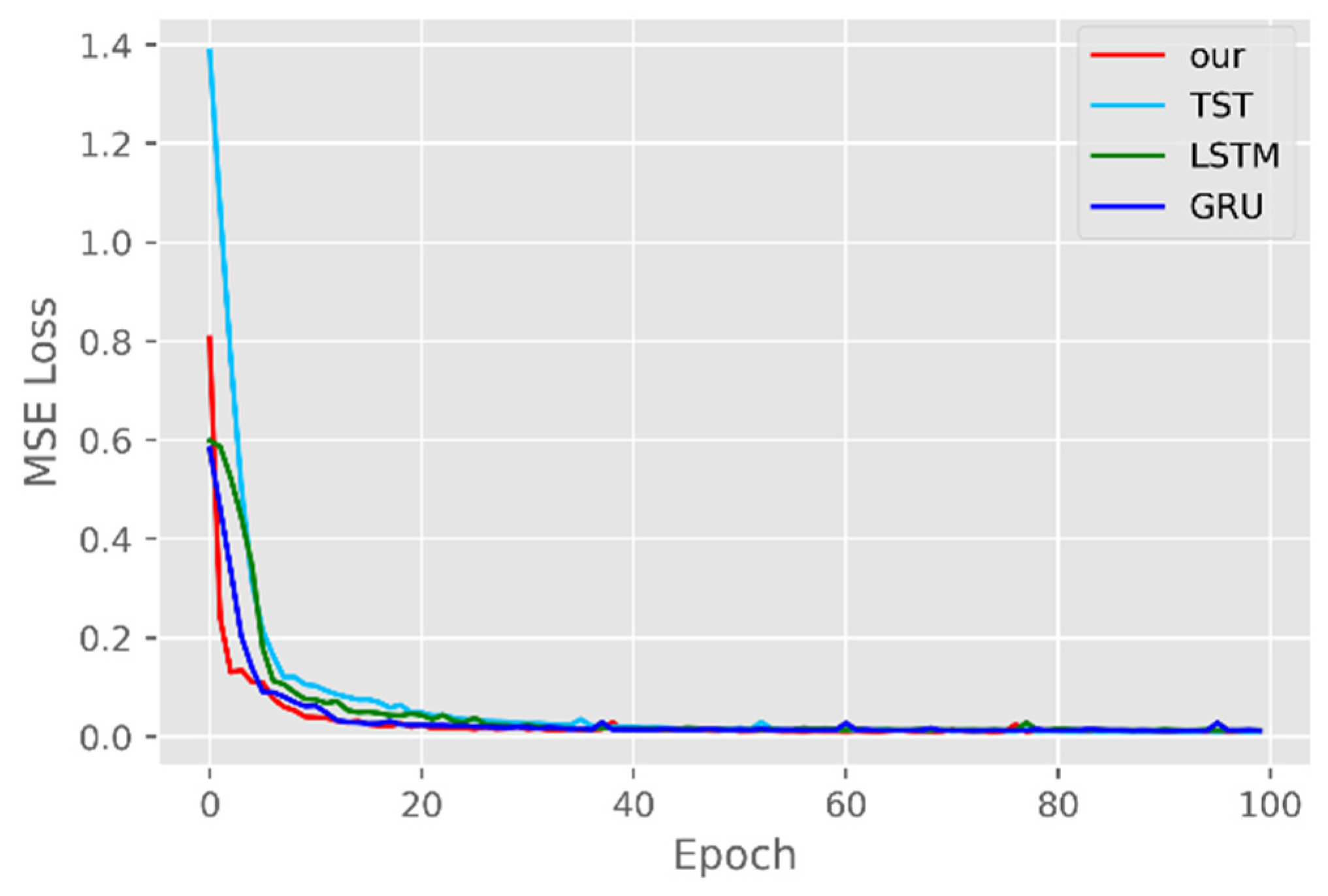
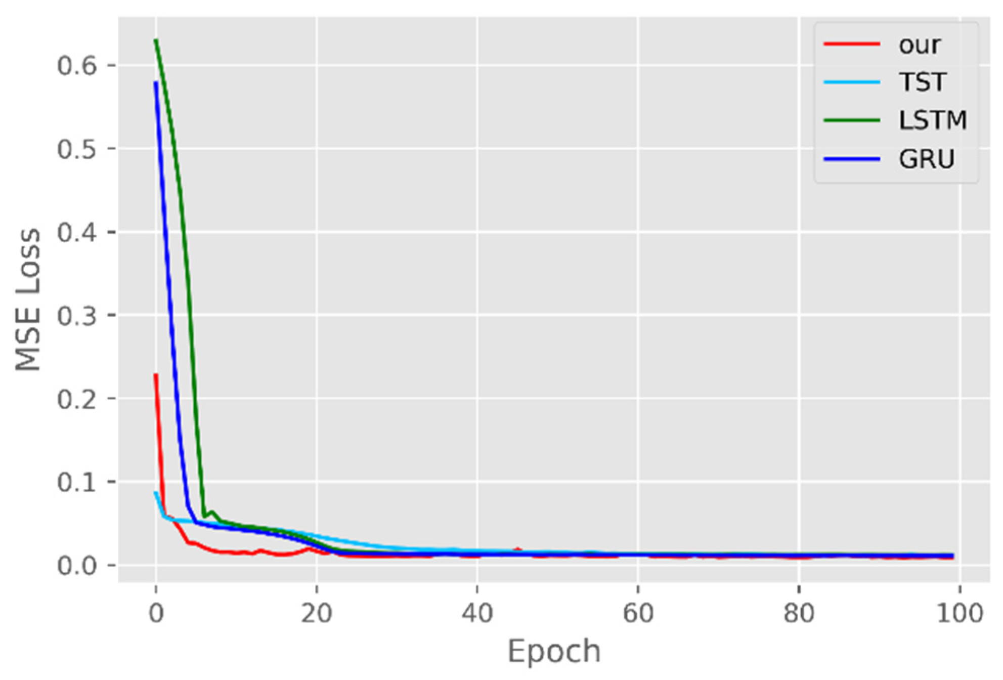
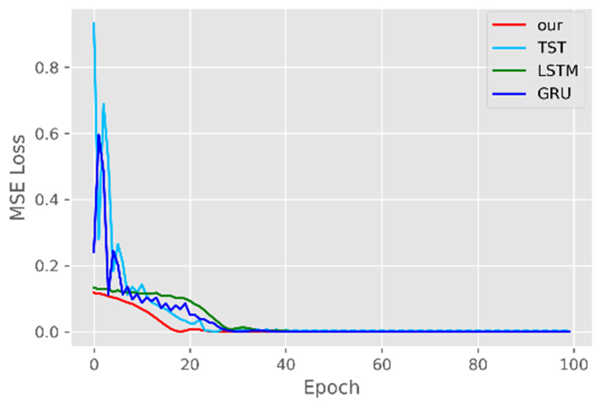
5.1. Comparison of Accuracy and Convergence of Models

We compare with three frontier DL models. We compare our findings to three states by analyzing the last 20% or 30% of days using $MAPE$ and $MSE$ score metrics. In graphs, we also explain how each model fits the observations differently. Due to an existing temporal correlation throughout the days, training converges and trains quickly in high population states such as NY, VA, and CA. However, not all models appear to completely reflect the pattern for states such as NY and VA. Only three states’ baseline data were compared, and then DL models are chosen to predict the remaining states’ outcomes.

The comparison of four models for CA cases, deaths and Vaccines is shown in Figure 3. Time-Series Transformer (TST), Long Short-Term Memory (LSTM), and Gated Recurrent Unit (GRU) all have higher MAPE and MSE ratings than our model. The model is better if the MAPE score is low. Specifically, our model has 20%, 16.6%, and 50% lower MAPE value drop in the prediction of the number of confirmations, deaths, and vaccinations, respectively, compared with the best TST model. Additionally, our model will have a 12.5% and 30% lower MSE value drop in the prediction of the number of confirmed diagnoses and deaths, and the number of vaccinations, respectively, compared to the best TST model.

Figure 4 shows a comparison of four models for NY cases, deaths, and vaccines. The MAPE and MSE ratings of TST, LSTM, and GRU are all higher than our model. If the MAPE score is low, the model is better. When compared to the best TST model, our model has a 10%, 33.33%, and 75% smaller MAPE value drop in predicting the number of confirmations, deaths, and vaccines, respectively. In addition, when compared to the best TST model, our model will have a 14.3% and 66.7% MSE value drop in the prediction of the number of verified diagnoses and deaths, as well as the number of vaccines.

Figure 5 compares four models for NY cases, deaths and vaccines. The MAPE and MSE values of TST, LSTM, and GRU are all superior to our model. If the MAPE score is low, the model is better. When compared to the best TST model, our model has an 8%, 16.7%, and 44.4% smaller MAPE value drop in the prediction of the number of confirmations, fatalities, and vaccines, respectively. In addition, when compared to the best TST model, our model will have a 2.5% and 12.5% lower MSE value drop in the prediction of the number of verified diagnoses and deaths, as well as the number of vaccines.

To further evaluate the predictive ability of our model for different data, the model training losses were compared. Figure 6, Figure 7, Figure 8, Figure 9, Figure 10 and Figure 11 show that our model has good convergence in the training process, and the overall performance is superior to TST, LSTM, and GRU models. The experimental results show that the model in this paper has good convergence for both metrics on all three data sets. Specifically, the overall stability of our model during training is high, and there are no large fluctuations in the later stages of training compared with the remaining three DL models. The stable training effect provides a guarantee for the improvement of prediction accuracy.

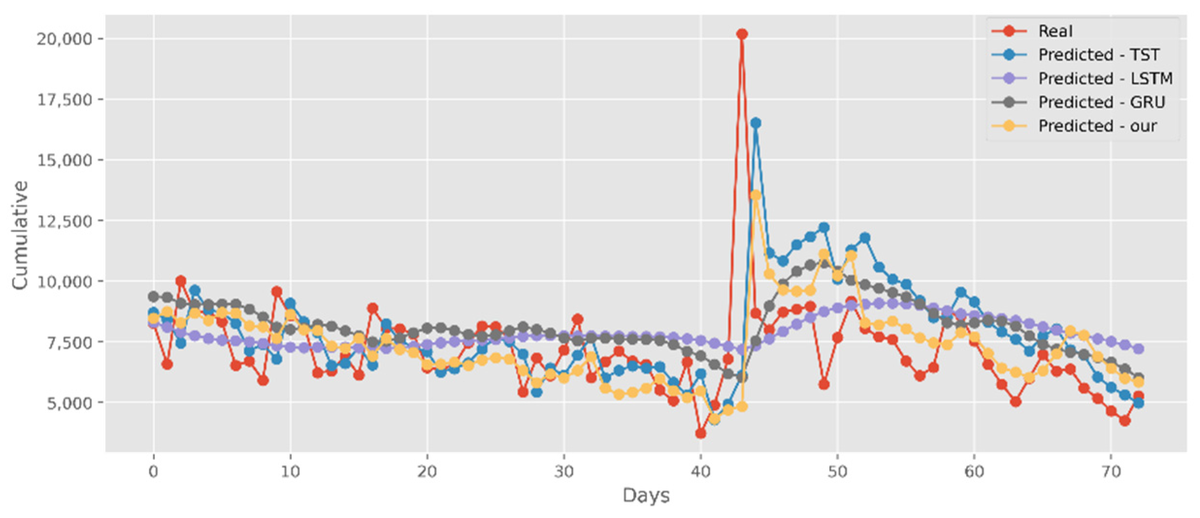
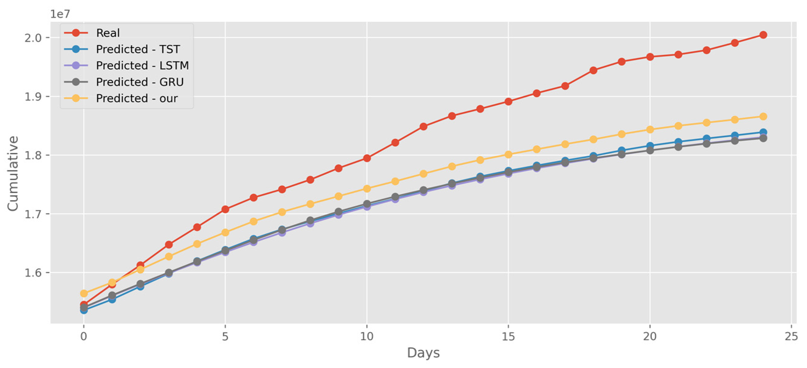
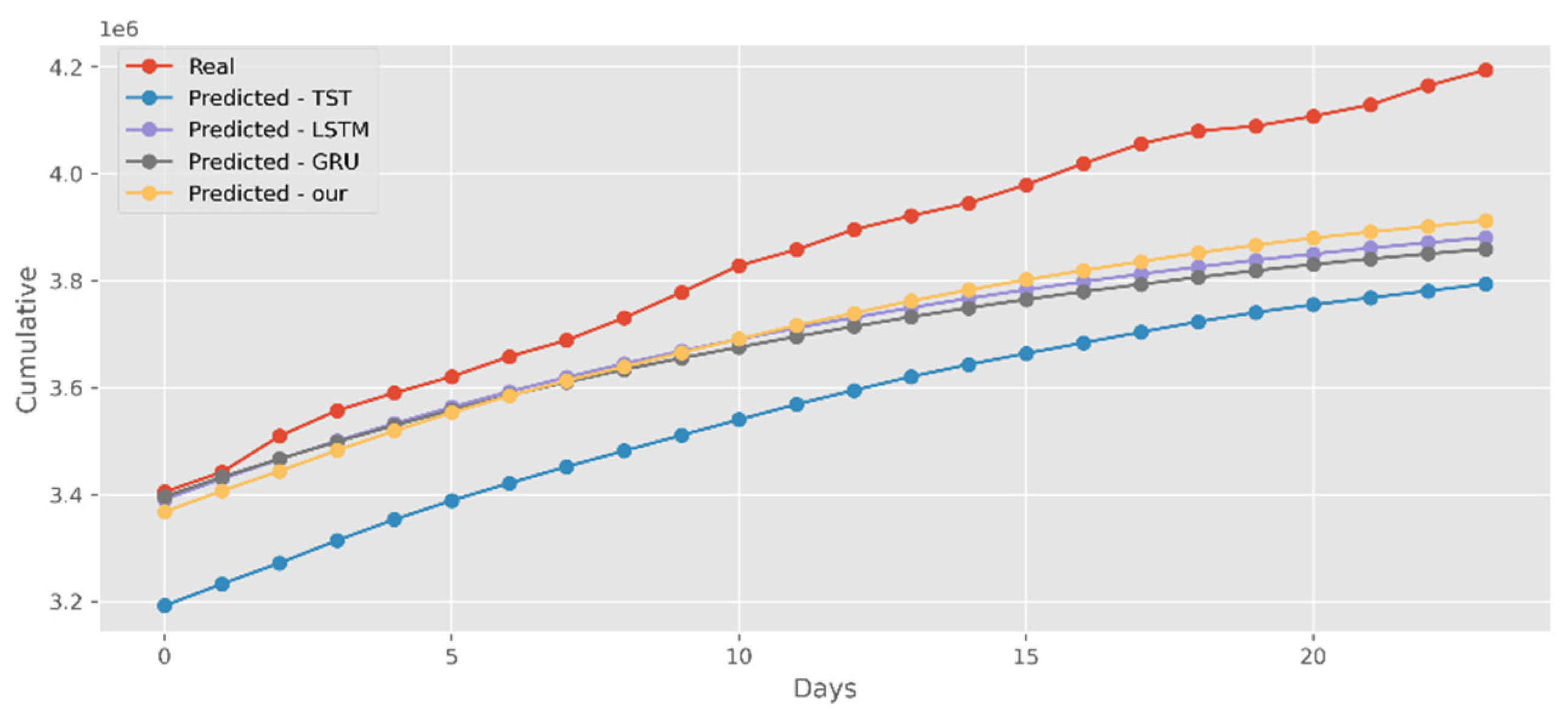
5.2. Forecasting the Number of Confirmed Cases

Figure 12 shows the predictions using three DL algorithms with respect to the actual test data set. The Y-axis in this graph shows the cumulative cases in CA. The X-axis shows the last two months: March and April 2021. Figure 13 also compares four algorithms by forecasting date ranges on NY test data sets. The Y-axis shows the daily cases of NY. Figure 14 also compares three algorithms by forecasting the date ranges in the VA test datasets. The Y-axis shows the daily cases of VA. Our model is the best option here as it also tried to capture the peaks, which is crucial in COVID-19 forecasting. It can be seen that the curve predicted by our model has a good fitting degree with the real data, and the overall deviation is small, which achieves the basic effect of prediction.

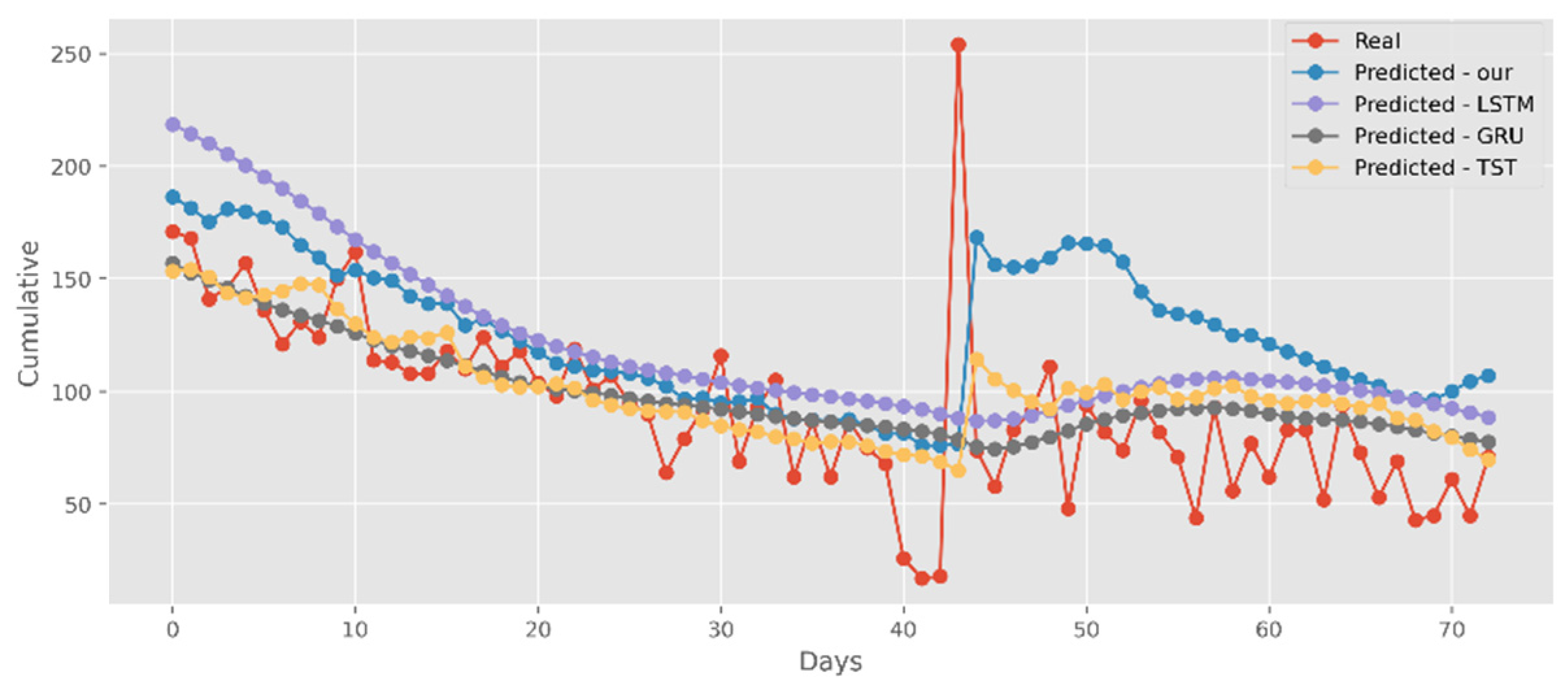
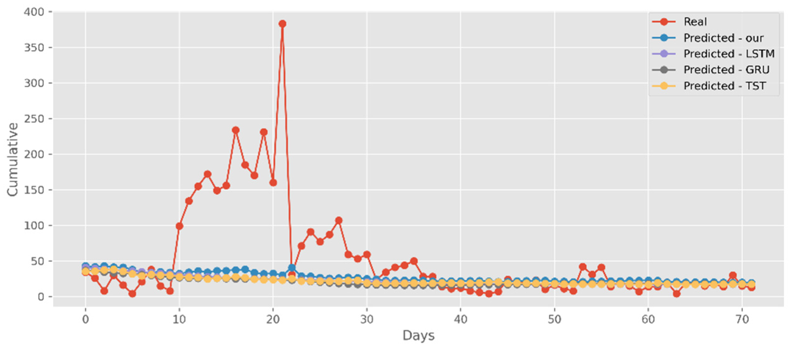
5.3. Forecasting the Number of Deaths

Figure 15 compares the predictions of three DL algorithms to the real-world test dataset of deaths. The Y-axis in this graph depicts the number of deaths every day in California. The X-axis represents the last two months of 2021: March and April. In addition, Figure 16 compares three methods by forecasting date ranges using NY’s test dataset. The Y-axis depicts the number of deaths in NY on a daily basis. By forecasting on VA’s test dataset date ranges, Figure 17 compares three algorithms. The Y-axis depicts the total number of VA deaths. Our model is unquestionably the best option here, as it attempted to capture the peaks, which is critical in COVID-19 predictions. It can be seen that the curve predicted by our model has a good fitting degree with the real data, and the overall deviation is minor, achieving the basic effect of prediction.

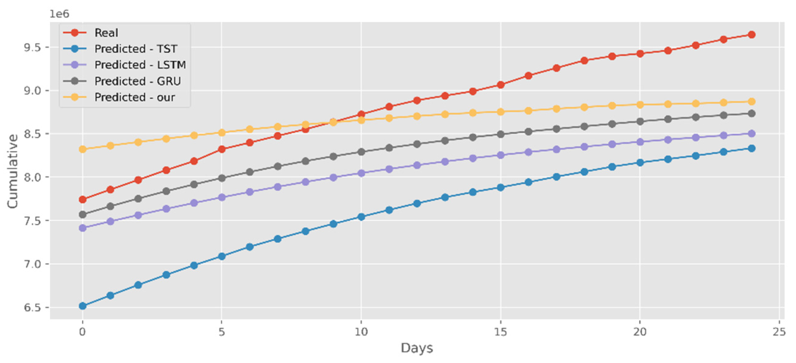
5.4. Forecasting the Number of Administrated Vaccine Doses

Figure 18 shows estimates using three different DL algorithms in relation to a real-world vaccination dataset. The y-axis of the graph depicts the cumulative vaccines in CA. On the X-axis, the latest 25 days are displayed. In addition, using NY’s test dataset, Figure 19 compares three techniques by forecasting date ranges. On the Y-axis, the cumulative immunizations of NY are displayed. In Figure 20, the date ranges of the VA test dataset are used to compare three algorithms. On the Y-axis are the VA vaccines. Because our model and Transformer are the most comparable to the real-world test dataset, they are the best choices. It can be seen that the curve predicted by our model fits the real data well, and the overall variance is tiny, achieving the basic impact of prediction.

6. Conclusions

In this work, we study and analyze COVID-19 data from three US states, including predicting the number of confirmed cases, deaths, and vaccinations in the future. To address the problems of low prediction accuracy and poor stability of existing DL models, we propose a hybrid model based on Transformer and GCN and compare it with DL models frequently used in time series prediction. In addition, we add the PDE technique to Transformer to improve the quality of the model when extracting time series information. The experimental results show that our proposed hybrid model outperforms frontier DL models such as TST, LSTM, and GRU in terms of model convergence and prediction effect. Compared with the powerful TST model, it has greater improvement in all indexes of MAPE and MSE, which provides better reference value for the prevention of infectious diseases.

References

1. Chan, J.F.W.; Yuan, S.; Kok, K.H.; To, K.K.W.; Chu, H.; Yang, J.; Xing, F.; Liu, J.; Yip, C.C.Y.; Poon, R.W.S.; et al. A familial cluster of pneumonia associated with the 2019 novel coronavirus indicating person-to-person transmission: A study of a family cluster. Lancet 2020, 395, 514–523. [Google Scholar] [CrossRef] [Green Version]
2. Roda, W.C.; Varughese, M.B.; Han, D.; Li, M.Y. Why is it difficult to accurately predict the COVID-19 epidemic? Infect. Dis. Model. 2020, 5, 271–281. [Google Scholar] [CrossRef] [PubMed]
3. Zhan, Z.; Dong, W.; Lu, Y.; Yang, P.; Wang, Q.; Jia, P. Real-time forecasting of hand-foot-and-mouth disease outbreaks using the integrating compartment model and assimilation filtering. Sci. Rep. 2019, 9, 2661. [Google Scholar] [CrossRef]
4. Scarpino, S.V.; Petri, G. On the predictability of infectious disease outbreaks. Nat. Commun. 2019, 10, 898. [Google Scholar] [CrossRef] [PubMed] [Green Version]
5. Miller, J.C. Mathematical models of SIR disease spread with combined non-sexual and sexual transmission routes. Infect. Dis. Model. 2017, 2, 35–55. [Google Scholar] [CrossRef] [PubMed]
6. Werkman, M.; Green, D.M.; Murray, A.G.; Turnbull, J.F. The effectiveness of fallowing strategies in disease control in salmon aquaculture assessed with an SIS model. Prev. Vet. Med. 2011, 98, 64–73. [Google Scholar] [CrossRef] [Green Version]
7. Fast, S.M.; Kim, L.; Cohn, E.L.; Mekaru, S.R.; Brownstein, J.S.; Markuzon, N. Predicting social response to infectious disease outbreaks from internet-based news streams. Ann. Oper. Res. 2018, 263, 551–564. [Google Scholar] [CrossRef] [PubMed]
8. Kim, T.H.; Hong, K.J.; Do Shin, S.; Park, G.J.; Kim, S.; Hong, N. Forecasting respiratory infectious outbreaks using ED-based syndromic surveillance for febrile ED visits in a Metropolitan City. Am. J. Emerg. Med. 2019, 37, 183–188. [Google Scholar] [CrossRef] [Green Version]
9. Rahimi, I.; Gandomi, A.H.; Asteris, P.G.; Chen, F. Analysis and Prediction of COVID-19 Using SIR, SEIQR, and Machine Learning Models: Australia, Italy, and UK Cases. Information 2021, 12, 109. [Google Scholar] [CrossRef]
10. Çolak, A.B. Prediction of infection and death ratio of CoVID-19 virus in Turkey by using artificial neural network (ANN). Coronaviruses 2021, 2, 106–112. [Google Scholar] [CrossRef]
11. Chimmula, V.K.R.; Zhang, L. Time series forecasting of COVID-19 transmission in Canada using LSTM networks. Chaos Solitons Fractals 2020, 135, 109864. [Google Scholar] [CrossRef]
12. Da Silva, D.B.; Schmidt, D.; da Costa, C.A.; Da Rosa Righi, R.; Eskofier, B. DeepSigns: A predictive model based on Deep Learning for the early detection of patient health deterioration. Expert Syst. Appl. 2021, 165, 113905. [Google Scholar] [CrossRef]
13. Çolak, A.B. An experimental study on the comparative analysis of the effect of the number of data on the error rates of artificial neural networks. Int. J. Energy Res. 2021, 45, 478–500. [Google Scholar] [CrossRef]
14. Torres, J.F.; Hadjout, D.; Sebaa, A.; Martínez-Álvarez, F.; Troncoso, A. Deep learning for time series forecasting: A survey. Big Data 2021, 9, 3–21. [Google Scholar] [CrossRef]
15. Shafiq, A.; Çolak, A.B.; Sindhu, T.N.; Lone, S.A.; Alsubie, A.; Jarad, F. Comparative Study of Artificial Neural Network versus Parametric Method in COVID-19 data Analysis. Results Phys. 2022, 38, 105613. [Google Scholar] [CrossRef]
16. Alali, Y.; Harrou, F.; Sun, Y. A proficient approach to forecast COVID-19 spread via optimized dynamic machine learning models. Sci. Rep. 2022, 12, 2467. [Google Scholar] [CrossRef] [PubMed]
17. Rahimi, I.; Chen, F.; Gandomi, A.H. A review on COVID-19 forecasting models. Neural Comput. Appl. 2021, 1–11. [Google Scholar] [CrossRef]
18. Kim, M.; Kang, J.; Kim, D.; Song, H.; Min, H.; Nam, Y.; Park, D.; Lee, J.G. Hi-covidnet: Deep learning approach to predict inbound COVID-19 patients and case study in South Korea. In Proceedings of the 26th ACM SIGKDD International Conference on Knowledge Discovery & Data Mining, Virtual Event, CA, USA, 6–10 July 2020; pp. 3466–3473. [Google Scholar]
19. Miralles-Pechuán, L.; Jiménez, F.; Ponce, H.; Martínez-Villaseñor, L. A methodology based on deep q-learning/genetic algorithms for optimizing COVID-19 pandemic government actions. In Proceedings of the 29th ACM International Conference on Information & Knowledge Management, Virtual Event, Ireland, 19–23 October 2020; pp. 1135–1144. [Google Scholar]
20. Shorten, C.; Khoshgoftaar, T.M.; Furht, B. Deep Learning applications for COVID-19. J. Big Data 2021, 8, 18. [Google Scholar] [CrossRef] [PubMed]
21. Farsani, R.M.; Pazouki, E. A transformer self-attention model for time series forecasting. J. Electr. Comput. Eng. Innov. 2021, 9, 1–10. [Google Scholar]
22. La Gatta, V.; Moscato, V.; Postiglione, M.; Sperli, G. An epidemiological neural network exploiting dynamic graph structured data applied to the COVID-19 outbreak. IEEE Trans. Big Data 2021, 7, 45–55. [Google Scholar] [CrossRef]
23. Cao, D.; Wang, Y.; Duan, J.; Zhang, C.; Zhu, X.; Huang, C.; Tong, Y.; Xu, B.; Bai, J.; Tong, J.; et al. Spectral temporal graph neural network for multivariate time-series forecasting. arXiv 2021, arXiv:2103.07719. [Google Scholar]
24. Nytimes. Coronavirus (COVID-19) Data in the United States. 2021. Available online: https://github.com/nytimes/covid-19-data (accessed on 8 June 2022).
25. Srk. Novel Corona Virus 2019 Dataset. 2021. Available online: https://www.kaggle.com/sudalairajkumar/novel-corona-virus-2019-dataset (accessed on 8 June 2022).
26. Edouard, M. State-By-State Data on COVID-19 Vaccinations in the United States. 2021. Available online: https://ourworldindata.org/us-states-vaccinations (accessed on 8 June 2022).
27. Vaswani, A.; Shazeer, N.; Parmar, N.; Uszkoreit, J.; Jones, L.; Gomez, A.N.; Kaiser, Ł.; Polosukhin, I. Attention is all you need. arXiv 2017, arXiv:1706.03762. [Google Scholar]
28. Bresson, X.; Laurent, T. Residual gated graph convnets. arXiv 2017, arXiv:1711.07553. [Google Scholar]
29. Wang, Y.; Chen, Z.B. Dynamic graph Conv-LSTM model with dynamic positional encoding for the large-scale traveling salesman problem. Math. Biosci. Eng. 2022, 19, 9730–9748. [Google Scholar] [CrossRef]
30. Ioffe, S.; Szegedy, C. Batch normalization: Accelerating deep network training by reducing internal covariate shift. In Proceedings of the International Conference on Machine Learning (ICML), Lille, France, 6–11 July 2015; pp. 448–456. [Google Scholar]
31. He, K.; Zhang, X.; Ren, S.; Sun, J. Deep residual learning for image recognition. In Proceedings of the IEEE Conference on Computer Vision and Pattern Recognition 2016, Las Vegas, NV, USA, 27–30 June 2016; pp. 770–778. [Google Scholar]
32. Hamilton, W.; Ying, Z.; Leskovec, J. Inductive representation learning on large graphs. Presented at Advances in Neural Information Processing Systems 30: Annual Conference on Neural Information Processing Systems 2017, Long Beach, CA, USA, 4–9 December 2017; pp. 1024–1034. [Google Scholar]
Figure 1. COVID-19 confirmed cases in the US.
Sustainability 14 10393 g001
Figure 2. Framework of model.
Sustainability 14 10393 g002
Figure 3. Comparison of MAPE and MSE score for CA cases, deaths and vaccines.
Sustainability 14 10393 g003
Figure 4. Comparison of MAPE and MSE score for NY cases, deaths and vaccines.
Sustainability 14 10393 g004
Figure 5. Comparison of MAPE and MSE score for VA vases, deaths and vaccines.
Sustainability 14 10393 g005
Figure 6. Comparison of training loss for CA cases and deaths.
Sustainability 14 10393 g006
Figure 7. Comparison of training loss for CA vaccines.
Sustainability 14 10393 g007
Figure 8. Comparison of training loss for NY cases and deaths.
Sustainability 14 10393 g008
Figure 9. Comparison of training loss for NY vaccines.
Sustainability 14 10393 g009
Figure 10. Comparison of training loss for VA cases and deaths.
Sustainability 14 10393 g010
Figure 11. Comparison of training loss for VA vaccines.
Sustainability 14 10393 g011
Figure 12. Comparison of COVID-19 prediction models of cases in CA.
Sustainability 14 10393 g012
Figure 13. Comparison of COVID-19 prediction models of cases in NY.
Sustainability 14 10393 g013
Figure 14. Comparison of COVID-19 prediction models of cases in VA.
Sustainability 14 10393 g014
Figure 15. Comparison of COVID-19 prediction models of deaths in CA.
Sustainability 14 10393 g015
Figure 16. Comparison of COVID-19 prediction models of deaths in NY.
Sustainability 14 10393 g016
Figure 17. Comparison of COVID-19 prediction models of deaths in VA.
Sustainability 14 10393 g017
Figure 18. Comparison of COVID-19 prediction models of vaccinated in CA.
Sustainability 14 10393 g018
Figure 19. Comparison of COVID-19 prediction models of vaccinated in NY.
Sustainability 14 10393 g019
Figure 20. Comparison of COVID-19 prediction models of vaccinated in VA.
Sustainability 14 10393 g020