
Fault Identification of Electric Submersible Pumps Based on Unsupervised and Multi-Source Transfer Learning Integration


Abstract
:1. Introduction
- (1)
- Combining multiple unsupervised learning methods to extract the anomaly scores (AS) generated by the unsupervised anomaly detection function as a richer representation of the data.
- (2)
- The source domain of multiple samples was obtained by random sampling while ensuring that a minority of faulty samples were adequately selected, thus guaranteeing that a smaller number of samples could be adequately trained to improve the perception and weight of faulty samples. Then, combining the source domain training set and the target domain test set, a weak classifier based on the conditional distribution probability distribution is built for obtaining the classification results of the respective samples.
- (3)
- The set of multiple weak classifiers is used to become a strong classifier to complete the classification recognition task.
2. Related Work
2.1. Unsupervised Feature Learning Methods
2.2. Transfer Learning Method
2.3. Weighted Balanced Distribution Adaptation Algorithm
2.4. Data Analysis
3. Algorithm Design
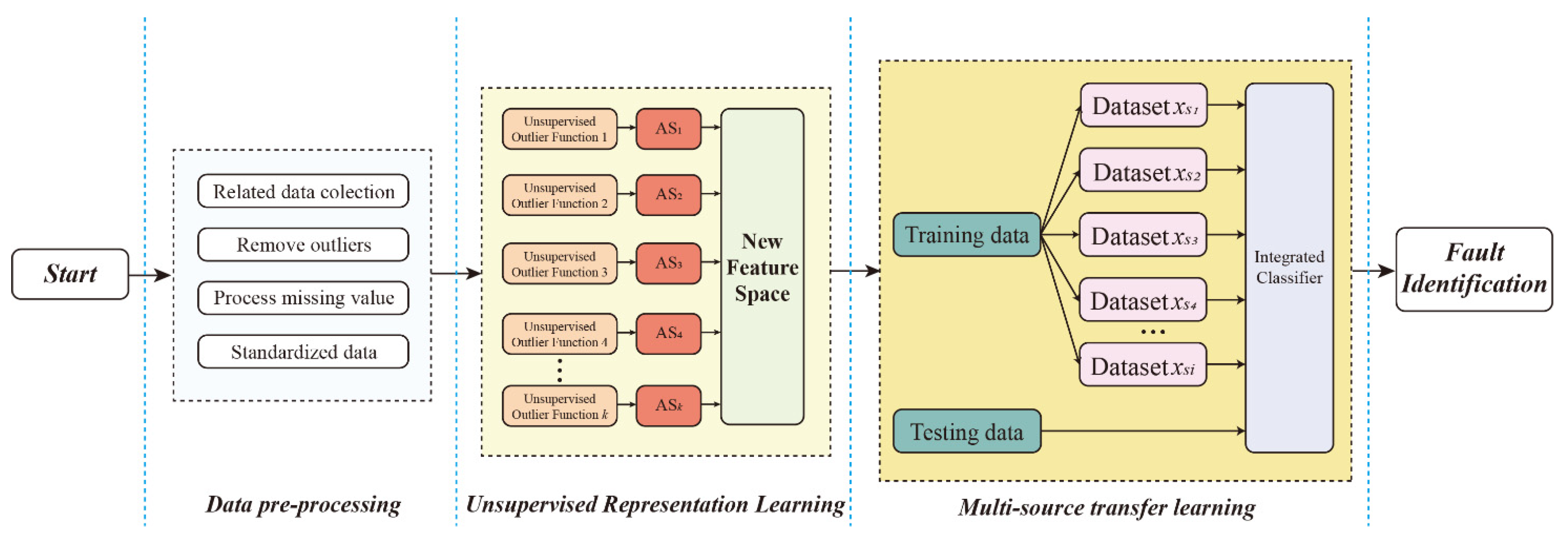
3.1. Method Flow
- Step 1: Data pre-processing of the collected data, including data cleaning, missing value filling, outlier processing, normalization, etc.
- Step 2: Inputting data into multiple unsupervised methods to construct a new feature space and enhance the information representative of a minority of fault samples.
- Step 3: Unduplicated random sampling of the training data while ensuring that a minority of faulty samples are adequately sampled.
- Step 4: Multiple training to obtain reliable base classifiers.
- Step 5: Multiple recognition results are integrated through multiple base classifiers to obtain the final recognition results.
3.2. Phase I: Data Pre-Processing
3.3. Phase 2: Unsupervised Representation Learning
3.4. Phase 3: Multi-Source Transfer Learning
4. Classifier Performance Evaluation Method
5. Experimental Analysis
5.1. Comparison of Classification Effects with and without Extraction of New Features
5.2. Effect of the Learning Framework
6. Discussion
7. Conclusions
Author Contributions
Funding
Institutional Review Board Statement
Informed Consent Statement
Data Availability Statement
Conflicts of Interest
References
- Langbauer, C.; Pratscher, H.P.; Ciufu, A.C.; Hoy, M.; Marschall, C.; Pongratz, R. Electric submersible pump behavior for pumping non-Newtonian fluids. J. Pet. Sci. Eng. 2020, 195, 107910. [Google Scholar] [CrossRef]
- Zhang, W.; Li, C.H.; Peng, G.L.; Chen, Y.H.; Zhang, Z.J. A deep convolutional neural network with new training methods for bearing fault diagnosis under noisy environment and different working load. Mech. Syst. Signal. Processing 2018, 100, 439–453. [Google Scholar] [CrossRef]
- Shen, L.; Chen, H.L.; Yu, Z.; Kang, W.C.; Zhang, B.Y.; Li, H.Z.; Yang, B.; Liu, D.Y. Evolving support vector machines using fruit fly optimization for medical data classification. Knowl. Based. Syst. 2016, 96, 61–75. [Google Scholar] [CrossRef]
- Ranawat, N.S.; Kankar, P.K.; Miglani, A. Fault Diagnosis in Centrifugal Pump using Support Vector Machine and Artificial Neural Network. J. Eng. Res. 2021, 9, 99–111. [Google Scholar] [CrossRef]
- Du, Y.C.; Du, D.P. Fault detection and diagnosis using empirical mode decomposition based principal component analysis. Comput. Chem. Eng. 2018, 115, 1–21. [Google Scholar] [CrossRef]
- Liu, J.Z.; Feng, J.; Gao, X.W. Fault Diagnosis of Rod Pumping Wells Based on Support Vector Machine Optimized by Improved Chicken Swarm Optimization. IEEE Access 2019, 7, 171598–171608. [Google Scholar] [CrossRef]
- Chen, Y.F.; Yuan, J.P.; Luo, Y.; Zhang, W.Q. Fault Prediction of Centrifugal Pump Based on Improved KNN. Shock Vib. 2022, 2021, 7306131. [Google Scholar] [CrossRef]
- Marins, M.A.; Barros, B.D.; Santos, I.H.; Barrionuevo, D.C.; Vargas, R.E.V.; Prego, T.D.; de Lima, A.A.; de Campos, M.L.R.; da Silva, E.A.B.; Netto, S.L. Fault detection and classification in oil wells and production/service lines using random forest. J. Pet. Sci. Eng. 2021, 197, 107879. [Google Scholar] [CrossRef]
- Chen, L.; Gao, X.W.; Li, X.Y. Using the motor power and XGBoost to diagnose working states of a sucker rod pump. J. Pet. Sci. Eng. 2021, 199, 108329. [Google Scholar] [CrossRef]
- Ji, S.X.; Pan, S.R.; Cambria, E.; Marttinen, P.; Yu, P.S. A Survey on Knowledge Graphs: Representation, Acquisition, and Applications. IEEE. Trans. Neur. Net. Lear. 2022, 33, 494–514. [Google Scholar] [CrossRef]
- Zhang, W.Y.; Yang, D.Q.; Zhang, S. A new hybrid ensemble model with voting-based outlier detection and balanced sampling for credit scoring. Expert. Syst. Appl. 2021, 174, 114744. [Google Scholar] [CrossRef]
- Sun, Y.T.; Ding, S.F.; Zhang, Z.C.; Zhang, C.L. Hypergraph based semi-supervised support vector machine for binary and multi-category classifications. Int. J. Mach. Learn. Cybern. 2022, 13, 1369–1386. [Google Scholar] [CrossRef]
- Solorio-Fernandez, S.; Carrasco-Ochoa, J.A.; Martinez-Trinidad, J.F. A review of unsupervised feature selection methods. Artif. Intell. Rev. 2020, 53, 907–948. [Google Scholar] [CrossRef]
- Kim, J.; Bukhari, W.; Lee, M. Feature Analysis of Unsupervised Learning for Multi-task Classification Using Convolutional Neural Network. Neural. Process. Lett. 2018, 47, 783–797. [Google Scholar] [CrossRef]
- Yepmo, V.; Smits, G.; Pivert, O. Anomaly explanation: A review. Data. Knowl. Eng. 2022, 137, 101946. [Google Scholar] [CrossRef]
- Pan, S.J.; Yang, Q.A. A Survey on Transfer Learning. IEEE. Trans. Knowl. Data. Eng. 2010, 22, 1345–1359. [Google Scholar] [CrossRef]
- Zhu, L.; Yang, J.T.; Ding, W.P.; Zhu, J.P.; Xu, P.; Ying, N.J.; Zhang, J.H. Multi-Source Fusion Domain Adaptation Using Resting-State Knowledge for Motor Imagery Classification Tasks. IEEE. Sens. J. 2021, 21, 21772–21781. [Google Scholar] [CrossRef]
- Gao, J.; Huang, R.; Li, H.X. Sub-domain adaptation learning methodology. Inf. Sci. 2015, 298, 237–256. [Google Scholar] [CrossRef]
- Jetti, H.V.; Ferrero, A.; Salicone, S. A modified Bayes’ theorem for reliable conformity assessment in industrial metrology. Measurement 2021, 184, 109967. [Google Scholar] [CrossRef]
- Jiang, K.; Jiang, Z.H.; Xie, Y.F.; Pan, D.; Gui, W.H. Abnormality Monitoring in the Blast Furnace Ironmaking Process Based on Stacked Dynamic Target-Driven Denoising Autoencoders. IEEE. Trans. Ind. Inform. 2021, 18, 1854–1863. [Google Scholar] [CrossRef]
- Villa-Perez, M.E.; Alvarez-Carmona, M.A.; Loyola-Gonzalez, O.; Medina-Perez, M.A.; Velazco-Rossell, J.C.; Choo, K.K.R. Semi-supervised anomaly detection algorithms: A comparative summary and future research directions. Knowl. Based. Syst. 2021, 218, 106878. [Google Scholar] [CrossRef]
- Kang, S.K. k-Nearest Neighbor Learning with Graph Neural Networks. Mathematics 2021, 9, 830. [Google Scholar] [CrossRef]
- Degirmenci, A.; Karal, O. Robust Incremental Outlier Detection Approach Based on a New Metric in Data Streams. IEEE. Access 2021, 9, 160347–160360. [Google Scholar] [CrossRef]
- Hu, Z.W.; Hu, Z.L.; Du, X.P. One-class support vector machines with a bias constraint and its application in system reliability prediction. AI. Edam. 2019, 33, 346–358. [Google Scholar] [CrossRef]
- Hariri, S.; Kind, M.C.; Brunner, R.J. Extended Isolation Forest. IEEE. Trans. Knowl. Data. Eng. 2021, 33, 1479–1489. [Google Scholar] [CrossRef] [Green Version]
- Shao, H.D.; Jiang, H.K.; Zhao, H.W.; Wang, F.A. A novel deep autoencoder feature learning method for rotating machinery fault diagnosis. Mech. Syst. Signal. Processing 2017, 95, 187–204. [Google Scholar] [CrossRef]
- Liberti, L.; Lavor, C.; Maculan, N.; Mucherino, A. Euclidean Distance Geometry and Applications. SIAM. Rev. 2014, 56, 3–69. [Google Scholar] [CrossRef]
- Jiang, H.; He, Z.; Ye, G.; Zhang, H.Y. Network Intrusion Detection Based on PSO-Xgboost Model. IEEE Access 2020, 8, 58392–58401. [Google Scholar] [CrossRef]
- Krishnakumari, K.; Sivasankar, E.; Radhakrishnan, S. Hyperparameter tuning in convolutional neural networks for domain adaptation in sentiment classification (HTCNN-DASC). Soft. Comput. 2020, 24, 3511–3527. [Google Scholar] [CrossRef]
- Han, S.; Choi, H.J.; Choi, S.K.; Oh, J.S. Fault Diagnosis of Planetary Gear Carrier Packs: A Class Imbalance and Multiclass Classification Problem. Int. J. Precis. Eng. Man. 2019, 20, 167–179. [Google Scholar] [CrossRef]
- Zhang, X.C.; Jiang, D.X.; Long, Q.; Han, T. Rotating machinery fault diagnosis for imbalanced data based on decision tree and fast clustering algorithm. J. Vibroeng. 2017, 19, 4247–4259. [Google Scholar] [CrossRef]
- Joshuva, A.; Kumar, R.S.; Sivakumar, S.; Deenadayalan, G.; Vishnuvardhan, R. An insight on VMD for diagnosing wind turbine blade faults using C4.5 as feature selection and discriminating through multilayer perceptron. Alexandria. Eng. J. 2020, 59, 3863–3879. [Google Scholar] [CrossRef]
- Kesemen, O.; Tiryaki, B.K.; Tezel, O.; Ozkul, E.; Naz, E. Random sampling with fuzzy replacement. Expert. Syst. Appl. 2021, 185, 115602. [Google Scholar] [CrossRef]
- Feng, S.; Keung, J.; Yu, X.; Xiao, Y.; Zhang, M. Investigation on the stability of SMOTE-based oversampling techniques in software defect prediction. Inform. Softw. Technol. 2021, 139, 106662. [Google Scholar] [CrossRef]
- Hassan, M.M.; Eesa, A.S.; Mohammed, A.J.; Arabo, W.K. Oversampling Method Based on Gaussian Distribution and K-Means Clustering. Cmc-Comput. Mater. Con. 2021, 69, 451–469. [Google Scholar] [CrossRef]
- Chen, Y.Y.; Zheng, W.Z.; Li, W.B.; Huang, Y.M. Large group activity security risk assessment and risk early warning based on random forest algorithm. Pattern. Recogn. Lett. 2021, 144, 1–5. [Google Scholar] [CrossRef]
- Xiang, C.; Ren, Z.J.; Shi, P.F.; Zhao, H.G. Data-Driven Fault Diagnosis for Rolling Bearing Based on DIT-FFT and XGBoost. Complexity 2021, 2021, 4941966. [Google Scholar] [CrossRef]
- Yan, C.; Li, M.X.; Liu, W. Transformer Fault Diagnosis Based on BP-Adaboost and PNN Series Connection. Math. Probl. Eng. 2019, 2019, 1019845. [Google Scholar] [CrossRef] [Green Version]
- Niu, K.; Zhang, Z.M.; Liu, Y.; Li, R.F. Resampling ensemble model based on data distribution for imbalanced credit risk evaluation in P2P lending. Inf. Sci. 2020, 536, 120–134. [Google Scholar] [CrossRef]
- Wang, W.P.; Wang, C.Y.; Wang, Z.; Yuan, M.M.; Luo, X.; Kurths, J.; Gao, Y. Abnormal detection technology of industrial control system based on transfer learning. Appl. Math. Comput. 2022, 412, 126539. [Google Scholar] [CrossRef]


| No. | Symbol | Variable Name (Unit) | No. | Symbol | Variable Name (Unit) |
|---|---|---|---|---|---|
| 1 | DLP | Daily liquid production (m3/day) | 9 | TLV | Test liquid volume (t) |
| 2 | WT | Wellhead temperature (°C) | 10 | DWP | Daily water production (m3/day) |
| 3 | TWV | Test water volume (m3/day) | 11 | DGP | Daily gas production (m3/day) |
| 4 | WGR | Water gas ratio (%) | 12 | DOP | Daily oil production (m3/day) |
| 5 | PC | Pump current (A) | 13 | WC | Water content (wt%) |
| 6 | PV | Pump voltage (V) | 14 | TOV | Test oil volume (t) |
| 7 | OP | Oil pressure (kPa) | 15 | GOR | Gas-oil ratio (%) |
| 8 | OGR | Oil gas ratio (%) | |||
| Working Conditions | Working Status | ||||
| Column leakage (1) | Lines break, disconnect, wear, and corrode, resulting in leaks. | ||||
| Overload pump stopping (2) | Overload current setting is not reasonable, the motor is impaired, the pump is mixed with impurities, etc. Overload shutdown occurs. | ||||
| Underload pump stopping (3) | Underload current setting is not reasonable, pump or separator shaft is broken due to insufficient fluid supply from the ground. | ||||
| Predicted for Positive Class | Forecast for Negative Class | |
|---|---|---|
| True for positive class | TP | FN |
| True for negative class | FP | TN |
| Classifier without Sampling | SVM_R_W: SVM with Gaussian function and imbalance weight |
| DT: Decision Trees [31] | |
| MLP: Multi-Layer perceptron [32] | |
| Classifiers with Sampling | R + SVM_R_W: Random sampling [33] + SVM_R_W |
| S + SVM_R_W: SMOTE [34] + SVM_R_W | |
| G + SVM_R_W: Gaussian Oversampling [35] + SVM_R_W | |
| Integrated Classification without Sampling | RF: Random Forest [36] |
| XGB: XGBoost [37] | |
| ADA: ADAboost [38] | |
| Integrated Classification with Sampling | R + XGB |
| REMDD |
| Methods | 1:1 | 1:2 | 1:5 | 1:10 | 1:15 | 1:20 | 1:30 | 1:50 | 1:100 | 1:200 |
|---|---|---|---|---|---|---|---|---|---|---|
| SVM_R_W | 0.9190 ± 0.03 | 0.9025 ± 0.01 | 0.8576 ± 0.00 | 0.8027 ± 0.01 | 0.6771 ± 0.00 | 0.6355 ± 0.00 | 0.5691 ± 0.01 | 0.5013 ± 0.20 | 0.3781 ± 0.01 | 0.1341 ± 0.00 |
| DT | 0.9201 ± 0.00 | 0.9165 ± 0.00 | 0.8211 ± 0.00 | 0.7557 ± 0.00 | 0.6013 ± 0.00 | 0.5261 ± 0.04 | 0.4971 ± 0.00 | 0.4043 ± 0.00 | 0.2239 ± 0.01 | 0.0963 ± 0.00 |
| MLP | 0.9284 ± 0.01 | 0.8433 ± 0.01 | 0.7287 ± 0.02 | 0.6562 ± 0.02 | 0.4870 ± 0.01 | 0.3873 ± 0.12 | 0.2431 ± 0.10 | 0.1141 ± 0.02 | 0.0692 ± 0.00 | 0.0072 ± 0.00 |
| RUS + SVM_R_W | 0.9112 ± 0.02 | 0.8452 ± 0.03 | 0.8461 ± 0.01 | 0.8233 ± 0.03 | 0.8081 ± 0.07 | 0.7433 ± 0.10 | 0.6523 ± 0.02 | 0.5508 ± 0.06 | 0.3066 ± 0.01 | 0.2036 ± 0.01 |
| S + SVM_R_W | 0.9338 ± 0.01 | 0.9008 ± 0.02 | 0.8601 ± 0.04 | 0.7930 ± 0.02 | 0.7330 ± 0.00 | 0.6964 ± 0.30 | 0.6156 ± 0.07 | 0.4364 ± 0.00 | 0.3272 ± 0.01 | 0.2513 ± 0.01 |
| G + SVM_R_W | 0.9510 ± 0.03 | 0.9364 ± 0.00 | 0.8272 ± 0.00 | 0.7772 ± 0.00 | 0.7073 ± 0.02 | 0.6234 ± 0.00 | 0.5672 ± 0.00 | 0.4655 ± 0.01 | 0.3770 ± 0.03 | 0.2041 ± 0.02 |
| RF | 0.9577 ± 0.00 | 0.9071 ± 0.00 | 0.8270 ± 0.11 | 0.7531 ± 0.14 | 0.6547 ± 0.00 | 0.5394 ± 0.01 | 0.4394 ± 0.01 | 0.3301 ± 0.00 | 0.2211 ± 0.03 | 0.1255 ± 0.05 |
| XGB | 0.9605 ± 0.03 | 0.9231 ± 0.01 | 0.9377 ± 0.00 | 0.8621 ± 0.08 | 0.7741 ± 0.01 | 0.6431 ± 0.00 | 0.5943 ± 0.10 | 0.3961 ± 0.01 | 0.2545 ± 0.00 | 0.1305 ± 0.01 |
| ADA | 0.9431 ± 0.08 | 0.9156 ± 0.00 | 0.8514 ± 0.05 | 0.8062 ± 0.12 | 0.7641 ± 0.07 | 0.7034 ± 0.02 | 0.6253 ± 0.00 | 0.4201 ± 0.02 | 0.3774 ± 0.09 | 0.3152 ± 0.04 |
| RUS +XGB | 0.9645 ± 0.00 | 0.9471 ± 0.00 | 0.9067 ± 0.00 | 0.8481 ± 0.01 | 0.8041 ± 0.07 | 0.7331 ± 0.05 | 0.5243 ± 0.00 | 0.4261 ± 0.00 | 0.3145 ± 0.04 | 0.2505 ± 0.01 |
| REMDD | 0.9205 ± 0.04 | 0.8723 ± 0.02 | 0.7737 ± 0.07 | 0.7551 ± 0.16 | 0.6741 ± 0.29 | 0.6031 ± 0.17 | 0.5143 ± 0.27 | 0.4561 ± 0.01 | 0.3345 ± 0.04 | 0.2805 ± 0.09 |
| UMTLA | 0.9821 ± 0.01 | 0.9644 ± 0.00 | 0.9245 ± 0.01 | 0.9121 ± 0.01 | 0.8841 ± 0.02 | 0.8554 ± 0.01 | 0.8104 ± 0.03 | 0.7715 ± 0.01 | 0.7443 ± 0.02 | 0.7042 ± 0.01 |
| Methods | 1:1 | 1:2 | 1:5 | 1:10 | 1:15 | 1:20 | 1:30 | 1:50 | 1:100 | 1:200 |
|---|---|---|---|---|---|---|---|---|---|---|
| SVM_R_W | 0.9212 ± 0.01 | 0.8933 ± 0.02 | 0.8311 ± 0.02 | 0.7559 ± 0.03 | 0.6912 ± 0.00 | 0.6051 ± 0.01 | 0.5334 ± 0.04 | 0.4231 ± 0.12 | 0.3581 ± 0.01 | 0.1401 ± 0.01 |
| DT | 0.9014 ± 0.00 | 0.9554 ± 0.01 | 0.7812 ± 0.01 | 0.7256 ± 0.01 | 0.6634 ± 0.02 | 0.5022 ± 0.01 | 0.5312 ± 0.02 | 0.4166 ± 0.01 | 0.2934 ± 0.01 | 0.1776 ± 0.20 |
| MLP | 0.8814 ± 0.00 | 0.8754 ± 0.03 | 0.7731 ± 0.01 | 0.7056 ± 0.01 | 0.6015 ± 0.01 | 0.5054 ± 0.02 | 0.4069 ± 0.11 | 0.3054 ± 0.23 | 0.2014 ± 0.05 | 0.1267 ± 0.00 |
| RUS + SVM_R_W | 0.9256 ± 0.01 | 0.9025 ± 0.01 | 0.8434 ± 0.01 | 0.7912 ± 0.01 | 0.7045 ± 0.01 | 0.6394 ± 0.01 | 0.5667 ± 0.11 | 0.4012 ± 0.01 | 0.3256 ± 0.08 | 0.2107 ± 0.02 |
| S + SVM_R_W | 0.9512 ± 0.02 | 0.8933 ± 0.02 | 0.8512 ± 0.01 | 0.7723 ± 0.03 | 0.7212 ± 0.00 | 0.6721 ± 0.02 | 0.5878 ± 0.01 | 0.4261 ± 0.04 | 0.3298 ± 0.02 | 0.2314 ± 0.01 |
| G + SVM_R_W | 0.9472 ± 0.02 | 0.9237 ± 0.01 | 0.8617 ± 0.03 | 0.8021 ± 0.03 | 0.7091 ± 0.02 | 0.6464 ± 0.12 | 0.5961 ± 0.02 | 0.4651 ± 0.03 | 0.3312 ± 0.01 | 0.2001 ± 0.02 |
| RF | 0.9225 ± 0.03 | 0.8731 ± 0.02 | 0.7937 ± 0.01 | 0.7451 ± 0.10 | 0.6641 ± 0.01 | 0.5931 ± 0.02 | 0.4742 ± 0.04 | 0.3961 ± 0.02 | 0.3045 ± 0.01 | 0.2205 ± 0.30 |
| XGB | 0.9675 ± 0.01 | 0.9014 ± 0.03 | 0.8943 ± 0.01 | 0.8347 ± 0.01 | 0.7671 ± 0.02 | 0.6746 ± 0.01 | 0.5859 ± 0.07 | 0.4673 ± 0.02 | 0.3611 ± 0.02 | 0.2522 ± 0.02 |
| ADA | 0.9431 ± 0.08 | 0.9156 ± 0.00 | 0.8514 ± 0.05 | 0.8062 ± 0.12 | 0.7641 ± 0.07 | 0.7034 ± 0.02 | 0.6253 ± 0.00 | 0.4201 ± 0.02 | 0.3774 ± 0.09 | 0.3152 ± 0.04 |
| RUS +XGB | 0.9633 ± 0.02 | 0.9179 ± 0.01 | 0.8672 ± 0.00 | 0.7613 ± 0.01 | 0.6821 ± 0.02 | 0.5483 ± 0.02 | 0.4638 ± 0.03 | 0.3732 ± 0.01 | 0.3215 ± 0.01 | 0.2621 ± 0.02 |
| REMDD | 0.9616 ± 0.01 | 0.9055 ± 0.02 | 0.8261 ± 0.01 | 0.7611 ± 0.13 | 0.6358 ± 0.21 | 0.5387 ± 0.14 | 0.4768 ± 0.20 | 0.4023 ± 0.05 | 0.3559 ± 0.01 | 0.2832 ± 0.04 |
| UMTLA | 0.9738 ± 0.02 | 0.9474 ± 0.01 | 0.9038 ± 0.00 | 0.8734 ± 0.01 | 0.8451 ± 0.01 | 0.8105 ± 0.03 | 0.7504 ± 0.02 | 0.7344 ± 0.02 | 0.6912 ± 0.02 | 0.6491 ± 0.01 |
Publisher’s Note: MDPI stays neutral with regard to jurisdictional claims in published maps and institutional affiliations. |
© 2022 by the authors. Licensee MDPI, Basel, Switzerland. This article is an open access article distributed under the terms and conditions of the Creative Commons Attribution (CC BY) license (https://creativecommons.org/licenses/by/4.0/).
Share and Cite
Yang, P.; Chen, J.; Wu, L.; Li, S. Fault Identification of Electric Submersible Pumps Based on Unsupervised and Multi-Source Transfer Learning Integration. Sustainability 2022, 14, 9870. https://doi.org/10.3390/su14169870
Yang P, Chen J, Wu L, Li S. Fault Identification of Electric Submersible Pumps Based on Unsupervised and Multi-Source Transfer Learning Integration. Sustainability. 2022; 14(16):9870. https://doi.org/10.3390/su14169870
Chicago/Turabian StyleYang, Peihao, Jiarui Chen, Lihao Wu, and Sheng Li. 2022. "Fault Identification of Electric Submersible Pumps Based on Unsupervised and Multi-Source Transfer Learning Integration" Sustainability 14, no. 16: 9870. https://doi.org/10.3390/su14169870