Abstract
The regularity and demand predictions of shared cycling are very necessary and challenging for the management and development of urban pedestrian and bicycle traffic. The bicycle-sharing system has the problem of spatial and temporal demand fluctuations and presents a very complex nonlinear regularity. The demand for shared bicycles is affected by many factors, including time, space, weather and the situation of COVID-19. This study proposes a new bicycle-sharing demand forecasting model (USTARN) based on the impact of COVID-19, which combines urban computing and spatiotemporal attention residual network. USTARN consists of two parts. In the first part, a spatiotemporal attention residual network model is established to learn the temporal correlation and spatial correlation of shared bicycle demand. The temporal characteristic branches of each spatial small region are trained, respectively, to predict the shared bicycle demand in batches in different regions and periods according to the historical data. In order to improve the prediction accuracy of the model, the second part of the model adjusts and redistributes the prediction results of the first part by learning other information of the city, such as the severity of COVID-19, weather, temperature, wind speed and holidays. It can predict the demand for shared bicycles in different urban areas in different periods and different severities of COVID-19. This study uses the order data of shared bicycles during the period of COVID-19 in 2020 obtained from the open data platform of Shenzhen municipal government as verification, analyzes the spatiotemporal regularity of the system demand and discusses the impact of the number of newly diagnosed patients and the daily minimum temperature on the demand for shared bicycles. The results show that USTARN can fully reflect time, space, the epidemic situation, weather and temperature, and the prediction results of the impact of wind speed and other factors on the demand for shared bicycles are better than the classical methods.
1. Introduction
Thanks to the development of the internet, many countries are actively developing artificial intelligence traffic management systems to help manage urban traffic and reduce resource waste more effectively [1]. Traffic prediction is an important part of intelligent transportation management, especially in densely populated cities with developed road networks, which can effectively allocate traffic resources and induce the direction of traffic flow [2], avoid congestion caused by large demand and concentrated demand in urban road networks and enhance the robustness of traffic. Due to the fluctuation of spatial and temporal demand in the shared bicycle system, it is necessary to accurately grasp the change of the use regularity of shared bicycles and the real-time demand, reduce resource waste and improve the accuracy and timeliness of shared bicycles delivery [3].
Before 2020, the internet bicycle sharing system led by Mobike in China developed rapidly and was widely used for the “last mile” travel problem. The relationship between the bicycle-sharing system and the bus system and the urban rail transit system was dominated by cooperation and connection, with little competition. Since 2020, with the occurrence of COVID-19, in order to reduce the crisis caused by the spread of the epidemic, the government has reduced services of the centralized public transport system, and the rental service of shared bicycles has shown an explosive growth. The traffic function of shared bicycles has changed, gradually changing from connecting other public transport modes to undertaking complete travel, becoming the main force of “one hour travel” [4].
Shared cycling has a high degree of time regularity, which is significantly different during holidays and working days [5], and there are obvious tidal characteristics near the subway station in residential areas [6]. Gao et al. [7] built a shared bicycle space model by combining land use information to analyze the distribution characteristics of strong source and sink points of the Beijing Mobike system and found that the distribution pattern of strong source and sink points has an obvious spatial-temporal heterogeneity.
Du et al. [8] used the random forest algorithm to find that the living area, the area of park green space and population size are positively correlated with the frequency of bicycle demand. Based on DBSCAN spatial clustering algorithm, Zhang [9], Yu [10], Hua [11], Matthew Douglas [12] and others found that the turnover rate of the shared bicycle system is low in the discrete areas of stations and high in the concentrated areas of stations. The areas with high cycle-sharing turnover are mainly residential areas and public transport stations nearby. Based on the above research, Sun et al. [13] used Matlab to build a BP neural network model based on the non-negative matrix factorization algorithm and identified four typical commuter travel modes and one non-commuter travel behavior, such as leisure and entertainment activities. Fricker [14] quantified the changes of non-motorized activities based on the Bayesian structured time series model, studied the impact of COVID-19 on non-motorized travel patterns and found that during the period of COVID-19, non-motorized activities in densely populated cities decreased, but non-motorized activities in non-densely populated markets increased.
Many scholars use traditional dynamic models to study the demand for shared bicycles, such as the multiple linear regression model [15,16], spatial regression model [17], logistic regression model [18] and evolutionary game theory [19]. El-Assi et al. [15] and Zhang et al. [16] found that the density of road network intersections, the integrity of single bicycle system infrastructure and the spatial distribution of transportation hubs have a significantly positive impact on the demand for bicycle sharing in Toronto, Canada. Sergio Guidon et al. [17] found that commuting accounted for a large proportion of bicycle-sharing trips in some cities in Switzerland, and its travel distance overlapped with the distance of traditional public transport and taxi services. Kapuku et al. [18] found that the demand for shared bicycles increased significantly when the bus required many transfers, and the traffic network was congested.
Machine learning is an excellent method to learn nonlinear laws. The iterative spectral clustering algorithm could classify and cluster the shared-bicycle sites [20], and combined with the label propagation algorithm and the gradient lifting regression tree, it could predict the total demand for Citigroup’s shared bicycle system in New York City, but the prediction accuracy was low. After combining the improved SS method and K-means method with the XGboost model [21], it was found that the prediction error of the model was less than that of Ref. [20]. The bimodal Gaussian inhomogeneous Poisson algorithm can be used to describe the intensity of shared bicycle demand and predict the demand for shared bicycles at the station by calculating the average of the number of bicycles borrowed and returned at the station [22]. Li et al. [23] and Qiao et al. [24] built an artificial neural network model to increase the matching rate between the supply and demand of users’ shared bicycles by 19% and proved that various weather factors and different time steps have different effects on the accuracy of the model. Although there were still a few stations with large prediction errors, the model combined with the random forest model and least-square regression algorithm could predict the number of shared bicycles retained at each single station in San Francisco, USA [25]. Xu et al. [26] used the improved LSTM-NNS method to predict the regional stock of shared bicycles within 30 min in Nanjing, China, and the prediction result was better than the other seven traditional prediction models, thus proving that the neural network model has a good prediction superiority.
Most of the existing studies used traditional methods to study the connection regularity of shared bicycles before 2019 and did not comprehensively consider other information of the city, so it is impossible to describe the impact of COVID-19 on the demand for shared bicycles and the structural changes in the traffic functions of shared bicycles. This study aims at building a data mining model based on COVID-19 and combined with urban computing and spatiotemporal attention residual network to build a shared bicycle demand prediction model, which not only predicts in the temporal and spatial dimensions but also integrates information from other dimensions of the city for a comprehensive prediction, so as to improve the accuracy of the prediction model.
2. Data and Analysis
2.1. Data and Study Area
The shared bicycle historical order data we use come from the Shenzhen municipal government open data platform, which is an open-source platform sponsored by the government to provide data for various researchers. Each shared bicycle is equipped with a GPS tracking system and a mobile intelligent leasing system. The operator can generate order data, including the time and longitude and latitude coordinates of the start and end nodes of the bicycle ID trip.
The 441 days of historical order data from 30 January 2020 to 15 April 2021 include 38.33 million orders, with a total of 29.11 million individual users and 0.5 million bicycles from Hello bike, Qingju bike and Meituan bike (formerly Mobike), respectively. The average daily usage of bicycles in the city reached 1.38 million trips, and the average daily turnover rate of bicycles was 3.5 times.
The study area is Shenzhen, as shown in Figure 1. The fields of order data include userID, orderID, shared bikeID, start time, start location, end time, end location and shared bicycle source. Each record can be modeled as two spatiotemporal events: start event and end event, with corresponding timestamp and spatial coordinate information.
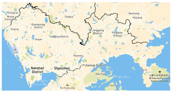
Figure 1.
Study area.
2.2. Preliminary Analysis of Spatial-Temporal Data
- (1)
- Spatial distribution characteristics
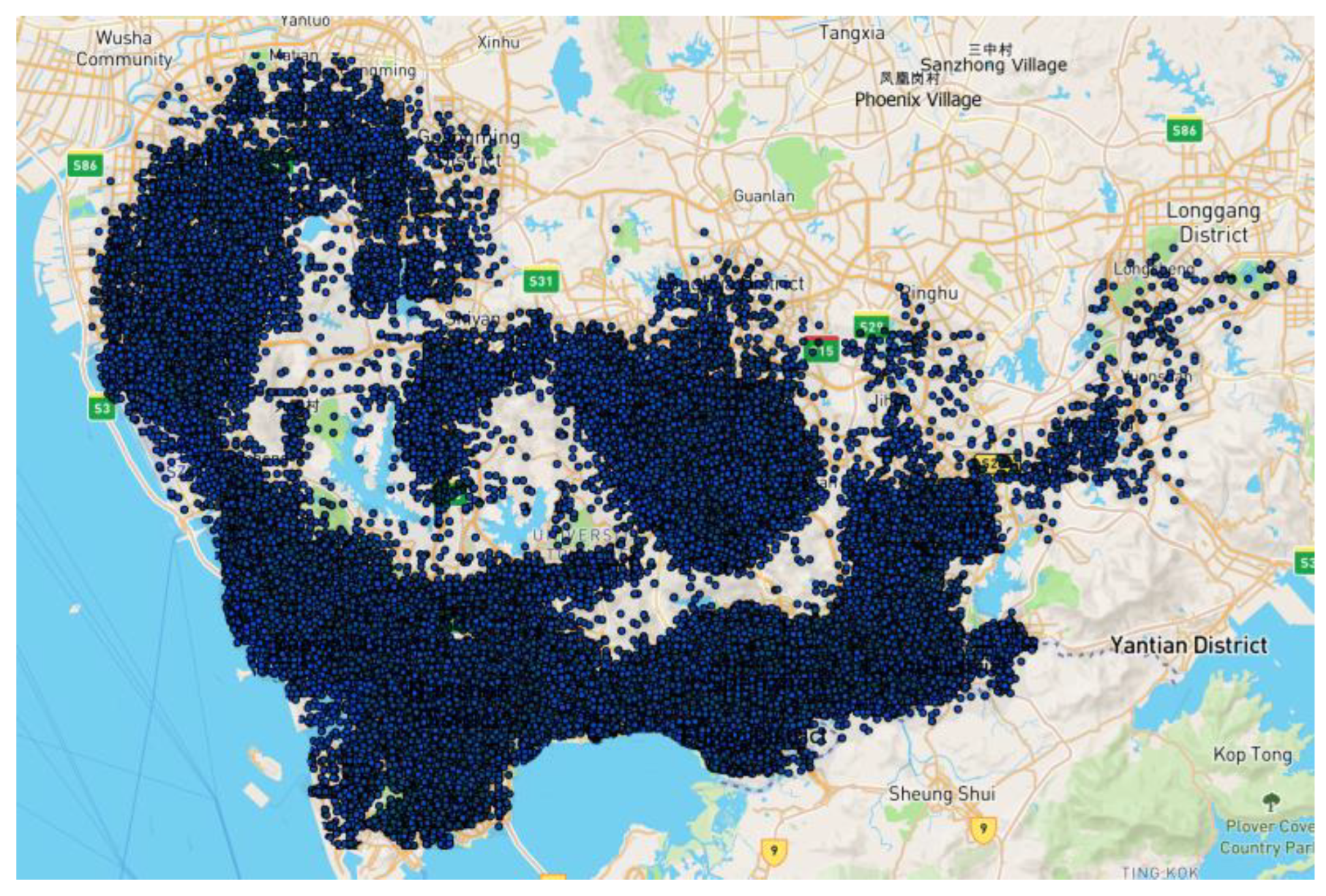
By filtering the location information of events in the order and matching it with geographic information through ArcGIS, the location of shared bicycles can be intuitively analyzed. Figure 2 shows the distribution of shared bicycles order starting events in Shenzhen on 13 April 2021.

Figure 2.
Distribution of the start event of shared bicycles.
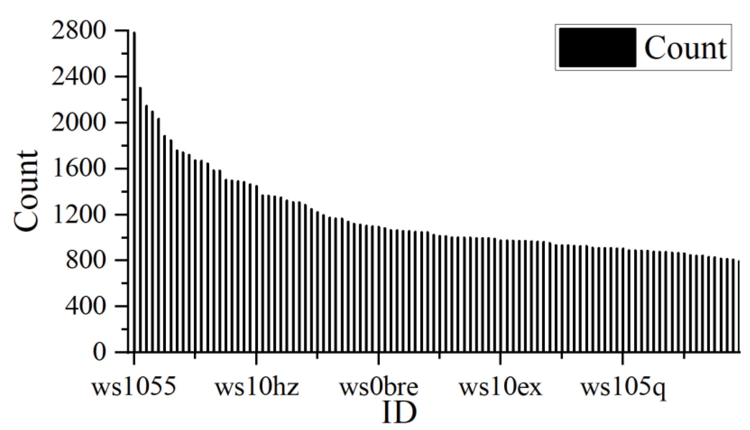
Using the geohash algorithm, Shenzhen is divided into districts with an accuracy of 6 and matched with the GPS coordinates of the start event of the order. Taking the number of start events per hour as the demand for shared bicycles per hour, the distribution of demand in different regions is obtained. As shown in Figure 3, the travel demand of the top 100 communities in Shenzhen at 8:00 on 13 April 2021 is shown, where the abscissa is the communityID, and the ordinate is the bicycle-sharing demand, most of which is in the residential areas and transportation hub areas and a small number of commercial areas.
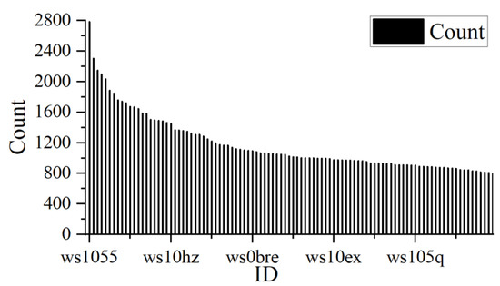
Figure 3.
Top 100 districts in bicycle-sharing demand.
- (2)
- Temporal distribution characteristics
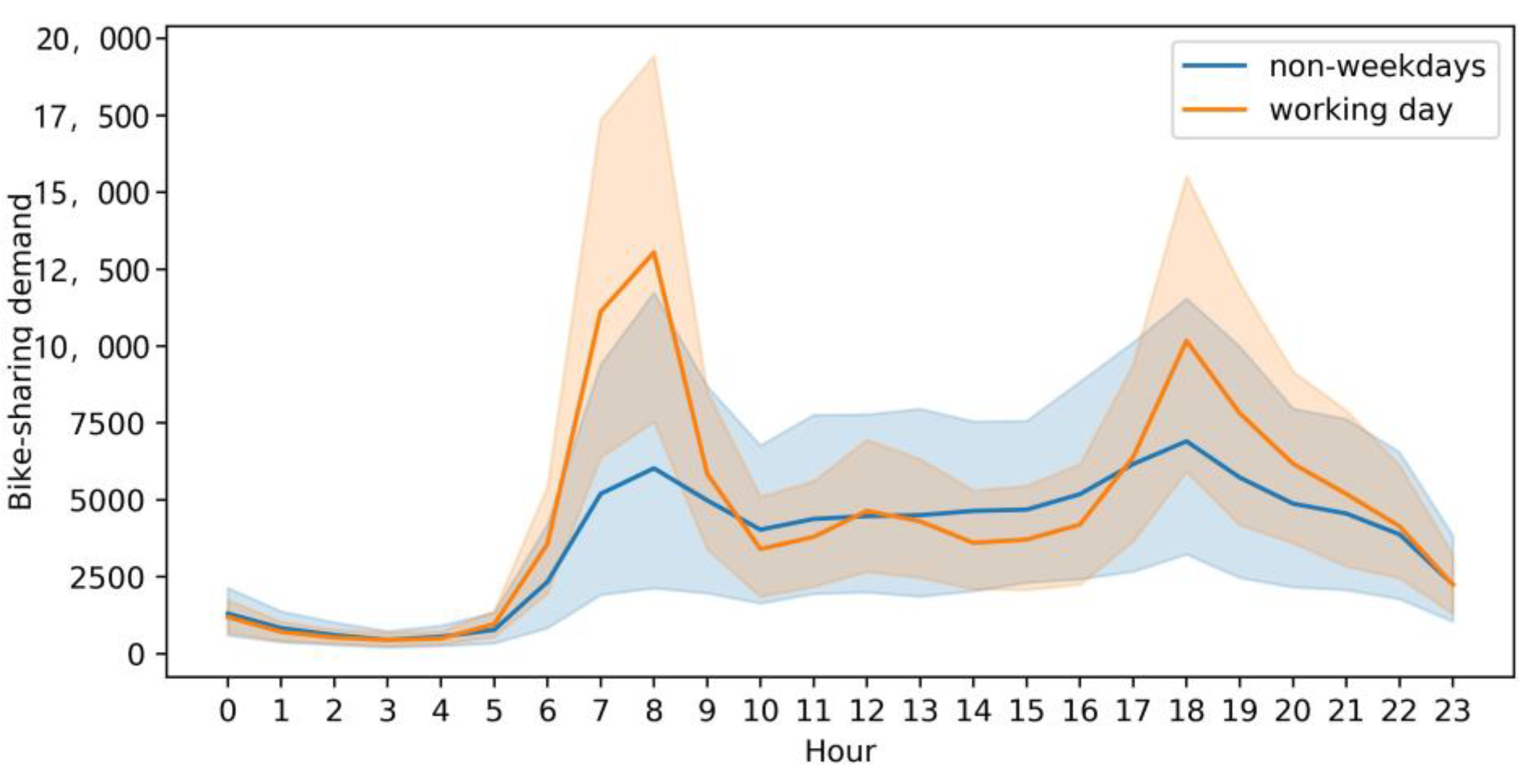
By using the Seaborn database and combining the time and calendar information of cycling starting events, we can obtain the correlation between the daily demand for shared bicycles and whether it is a working day, as shown in Figure 4, where the abscissa is 24 h per day, and the ordinate is the demand for bicycle sharing. We found that the distribution of daily bicycle-sharing demand is saddle shaped. The demand at daytime is higher than that at night time. The time distribution is more uneven on weekdays. The distribution of bicycle-sharing demand on non-weekdays is relatively uniform, without significant heterogeneity.

Figure 4.
Bicycle-sharing demand with different time attributes.
- (3)
- Other urban factors’ characteristics
We analyzed the correlation between the daily increase in COVID-19 patients and the historical data of bicycle-sharing orders obtained by the center for Disease Control and prevention of Shenzhen City, as shown in Figure 5, where the abscissa is the daily confirmed number of new COVID-19 cases, and the ordinate is the bicycle-sharing demand. The situation where the demand is 0 is due to the bicycle-sharing data corresponding to the new COVID-19 cases not being counted. The results showed that when there was an epidemic, the demand for shared bicycles sharply increased compared with that when there was no epidemic, and it reached a peak when the number of new patients per day was eight–nine. However, due to the strict control measures in Shenzhen, we cannot conduct a correlation analysis of when the number of new patients was more than 10 per day.
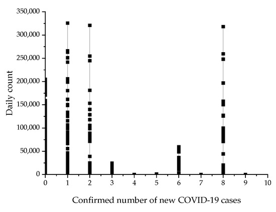
Figure 5.
Impact of epidemic on demand.
In addition, we also analyzed the correlation between the 441-day weather record data in Shenzhen obtained by the Shenzhen Meteorological Bureau and the shared bicycles historical order data, as shown in Figure 6. The abscissa is the maximum temperature of the day, and the ordinate is the bicycle-sharing demand of the day. The situation where the demand is 0 is due to the bicycle-sharing data corresponding to the temperature not being counted. The daily maximum temperature in Shenzhen ranges from 7 °C to 37 °C. Through statistical analysis, we found that the demand is small when the maximum temperature is lower than 19 °C and higher than 31 °C; when the daily maximum temperature is 20~30 °C, the average daily demand for bicycle sharing is large; and when the daily maximum temperature is 23 °C, the demand reaches a peak.
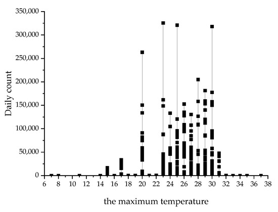
Figure 6.
Impact of temperature on demand.
3. Methodology
3.1. Definition of Time Step
Since the time step of the data of bicycle-sharing demand per hour per cell after processing is 1 h, we define the time step named c as 1 and take the first time node in the data as the time starting point. Define the demand in the t-th time step of cell i as Xi(t) ∈ R, the total historical demand in the historical T time step of time node i as Xi = {Xi(j)|j = 1, 2, …, T} and the total historical demand of N nodes as Xn = {Xn|n = 1, 2, …, N}.
3.2. Problem
Through the given historical order data X, the bicycle-sharing demand of each grid in the future TX time after the t-th time step is predicted in batches.
3.3. USTARN Model
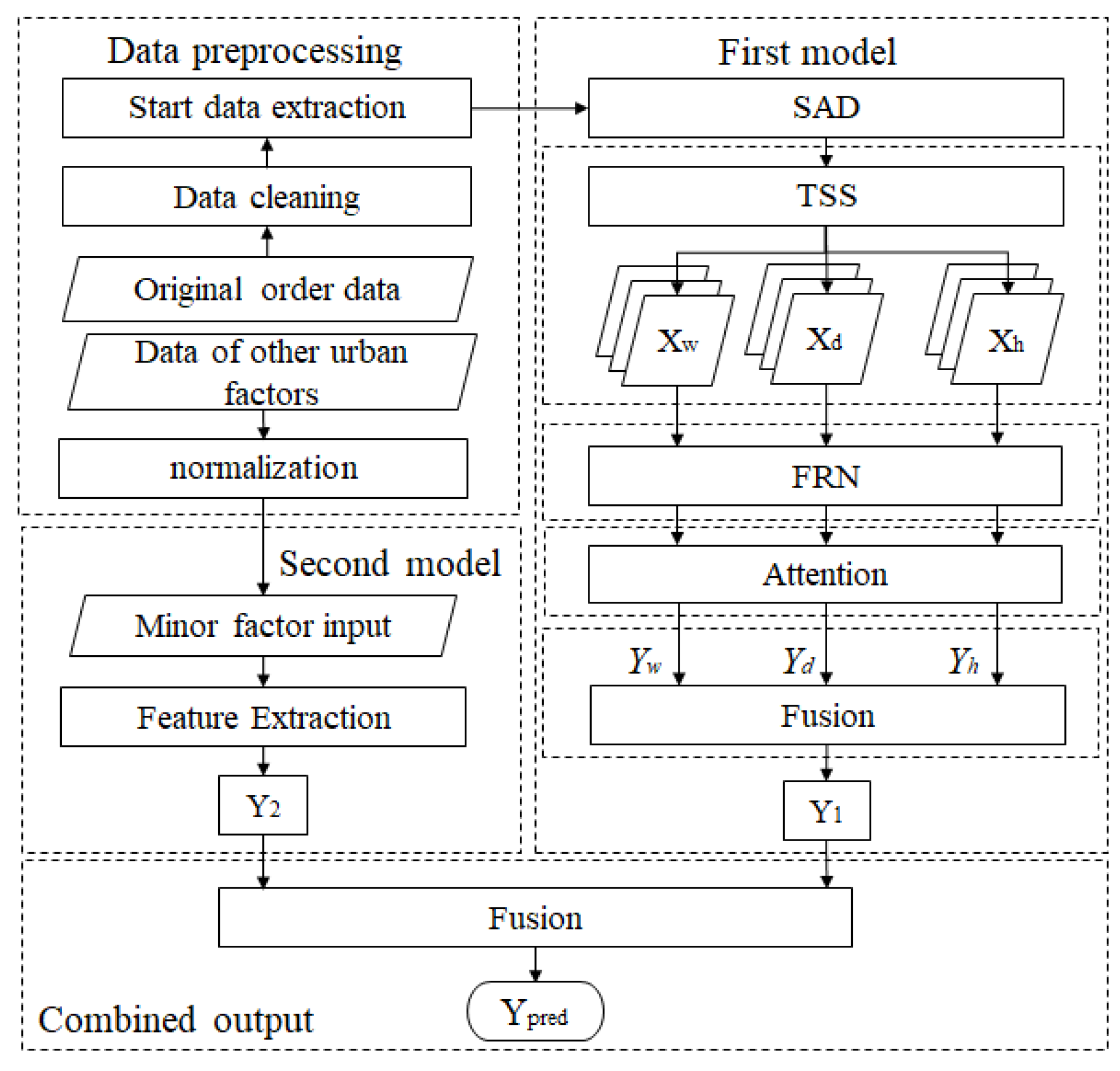
Figure 7 shows the overall structure of the USTARN model. The model includes four parts: the data processing part, the first prediction model, the second prediction model and the final prediction. The data processing part is to extract the starting event from the historical data of bicycle sharing and normalize other urban information. The first prediction model is the spatiotemporal attention residual network, including the spatial division module (SAD), time series division module (TSS), filled residual network (FRN) combined with the attention mechanism (Attention) and the fusion prediction (Fusion). The second prediction model is the prediction of other urban factors, and the final prediction is the combined output.
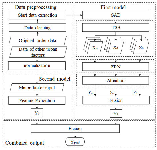
Figure 7.
The framework of USTARN.
- (1)
- Data processing
We extract the start timestamp and spatial coordinates of each order from the shared bicycle historical order data as the start event set and input it into the first prediction model. Because the different units of other urban factors, such as the daily increase in COVID-19 patients and existing number of COVID-19 cases, the maximum and minimum temperature, wind speed, weather conditions, working day status, etc., will affect the effect of prediction, the data of other urban factors will be normalized and input into the second prediction model.
- (2)
- The first prediction model
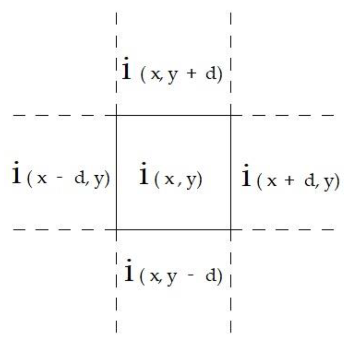
Spatial area division (SAD). Most of the existing studies only predict the traffic demand of all sections or a fixed section in a certain period of time, and the prediction results are relatively weak [27]. In order to achieve more accurate batch demand forecasting for all regions in a certain period of time, we set the step d with longitude as the y-axis and latitude as the x-axis in combination with the actual situation, divide a large area to be measured into many cells according to longitude and latitude, and define the coordinate value of cell i as (x, y), as shown in Figure 8.
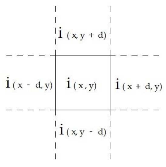
Figure 8.
Spatial area division.
Time series segmentation (TSS). The essence of traffic data is periodic time series data [28]. According to the relevant literature in the spatiotemporal field [29], a small number of critical data can determine a small number of future data. Therefore, combined with the asynchronous long-term characteristics, the comprehensive prediction of future demand can improve the prediction accuracy of the model. We use three segments with different timestamp lengths to predict the bicycle-sharing demand in the next hour. We define Tx = 1 for the segment to be tested, c = 1 for the segment Yh adjacent to 1 h, c = 24 for the segment Yd adjacent to 1 day and c = 168 for the segment Yw adjacent to 1 week. As shown in Figure 9, the model cuts the input data into the above three segments according to the time series.
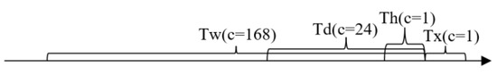
Figure 9.
Time series segmentation.
Filled residual network (FRN). Some scholars find that the training process of traditional machine-learning methods is complicated and time consuming, so deep learning is introduced into the field of traffic flow prediction, such as graph convolution [30] and various artificial neural networks [20,21,22,23]. However, the stack of convolutional layers is prone to gradient explosion and gradient disappearance, which affects the model accuracy. Therefore, scholars defined a new residual network method. In Formula (1), the input parameter x was added to the learning result F(x) of this layer to obtain the residual network result H(x) during data processing. Each iteration of the model was a cross-layer connection, so as to better preserve the original parameter characteristics and avoid gradient explosion or gradient disappearance [31,32,33].
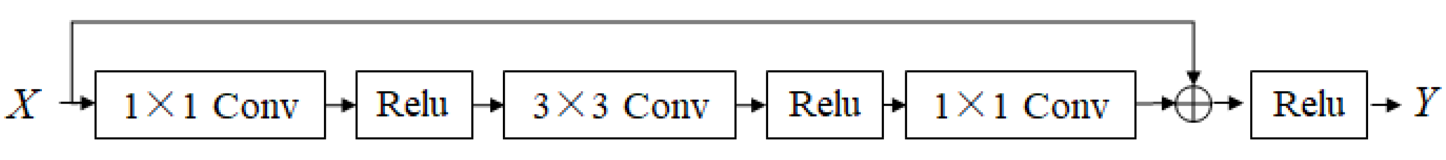
We use three residual networks to learn the data of three time series fragments. As shown in Figure 10, each network structure is composed of two residual layers, and each residual layer is composed of three convolution layers and three activation functions. Relu is the activation function used to ensure the convergence speed of the network and prevent the over-fitting phenomenon.
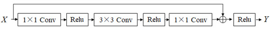
Figure 10.
Residual network structure.
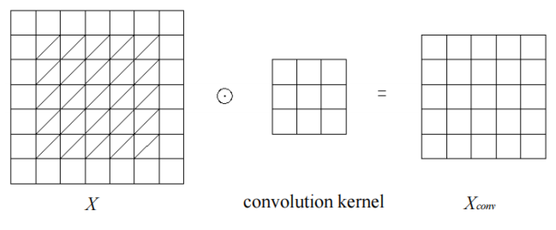
Convolution unit (Conv). Due to the large urban area, the number of cells after SD is also large, and the distance interval between any two cells is also large. Although the interaction between regions near each other is the main influence, the interaction between regions far away from each other cannot be ignored. Convolution operation is a very good method to capture the spatial dependence of two points [34]. As shown in Figure 9, we first use convolution kernel parameters of size 1 × 1 check data for dimensionality reduction to reduce the influence of noise points, then use convolution kernel parameters of size 3 × 3 to extract data features and finally use convolution kernel parameters of size 1 × 1 to restore data dimensions. In addition, we ensure the integrity of data transmission through the edge filling. As shown in Figure 11, the input information is filled with a circle of blank information. is the Hadamard product multiplied between block elements. Xconv is the output of convolution.
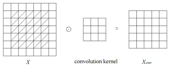
Figure 11.
Convolution.
Attentional mechanism (Attention). The attention mechanism includes squeezing, stimulating and weighting. The information with the input features W × L and channel number C; after passing through the attention unit, the size and channel number of the output feature remain unchanged, but the weight ratio between the pixels changes. The weight of the feature map of useful information becomes larger. The spatiotemporal theory proves that the shape and structure of a future frame of data can be determined by the preceding key frames of data, so we input the three demand prediction matrices output by the FRN network into the unit of attention and redistribute the weight of the three prediction results according to different time order dependences.
Fusion prediction (Fusion). Formula (2) describes the flow prediction matrix Yh, Yd and Yw of different features of time output by the attentional mechanism through a fully connected layer to obtain the demand prediction matrix Y1 based on the historical order data of shared bicycles.
where , and are three trainable parameters representing the influence of adjacent hour, adjacent day and adjacent week, respectively. is the Hadamard product.
- (3)
- The second prediction model
In Section 2.2, we found that there is a significant correlation between shared-bicycle cycling and weather, temperature, epidemic diseases, holidays, etc., so the one-to-one prediction of demand based on spatiotemporal characteristics is not consistent with reality. A comprehensive many-to-one prediction should be made based on urban conditions and other influencing factors of the city.
We processed the data of other factors in the city in the first step and obtained a feature matrix with m features and the same time dimension as the first model. Then, the feature matrix was embedded in a fully connected layer. The date attribute in the feature was known, while the weather and epidemic were unknown. By matching the calendar, the model obtained the information of working days and holidays. The model uses the weather with the temporal characteristic of Xh to approximately predict the weather at Tx and the epidemic data with the temporal characteristic of Xw to predict the epidemic at Tx. Finally, the result of the second model Y2 is output.
- (4)
- The final prediction
Through a fully connected layer, we used the characteristic matrix Y2 of other factors in the city predicted by the second model to study parameters and adjust the demand matrix Y1 of shared bicycles predicted by the first model and then output the final result matrix Ypred of demand prediction for each small area in the future Tx time.
4. Experiments
In order to evaluate and verify the model, the data sets of shared bicycles in Shenzhen and other factors in Shenzhen introduced in Section 2 are used for comparative case analysis of prediction.
4.1. Data Set Preprocessing
We used the 394-day historical order data of shared bicycles in the Shenzhen municipal government data open platform to produce statistics on the rental amount in hours, and a total of 100,896 h of shared bicycles’ demand data were input into the first model.
We used the data set of other factors in Shenzhen with the same time dimension as the input of other characteristics of the city into the second model. It included the daily number of newly confirmed COVID-19 cases and the number of confirmed COVID-19 cases on that day obtained by the Shenzhen CDC, the minimum temperature, maximum temperature, weather, wind speed on that day obtained by the Shenzhen Meteorological Bureau and whether the day is a working day based on the calendar. In order to eliminate the adverse effects of these data on the final prediction, the sklearn database was used to normalize the other urban data sets. Table 1 shows examples of the other normalized urban data sets.

Table 1.
Examples of other data preprocessing in cities.
4.2. Settings
SAD. Shenzhen is in the east longitude −113°46′~114°37′, north latitude 22°27′~22°52′. Figure 12 describes that we divide the longitude range of Shenzhen into 32 equal parts (abscissa) and the latitude range into 16 equal parts (ordinate) according to the longitude and latitude range. The master plan is divided into 512 small areas.
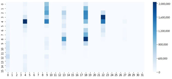
Figure 12.
Grid heat map of bicycle-sharing demand in a certain period.
SST. We take the first time node of the data set as the starting point to calculate the bicycle-sharing demand of each small area when c = 1 and divide the data set into the adjacent hour data segment Xh, the adjacent nearest day data segment Xd and the adjacent week data segment Xw.
The rest. We divide the data set into the training set, the verification set and the test set according to the ratio of 7:1:2. Then, we use Adam [35] as the model optimizer, set the prediction time step to 1 h, the number of iterations to 50, use the average absolute percentage error as the loss function (Formula (3)) and take the 118-th area as the output example of the test set.
where Ypred,i is the predicted demand matrix of the i-th region, and Ytru,i is the real demand matrix of the i-th region.
4.3. USTARN Experiments
Experiment A. In order to explore the influence of different residual network depths in the first model on the prediction accuracy of the overall model, we changed the number of residual network layers to conduct the experiments.
Experiment B. In order to prove that the USTARN model has a higher prediction accuracy and superiority than the USTRN model without the attention mechanism, we conducted a comparative experiment between the USTRN model and the USTARN model.
Experiment C. In order to prove the necessity and superiority of the second model, we conducted experiments to compare the prediction results without other characteristics of the city with the residual prediction results of USTARN.
4.4. Baselines
We compared our model with the following three baselines:
- (1)
- S-LSTM [27]: A long-term and short-term prediction model based on time series segmentation. S-LSTM adds the time series segmentation module on the basis of a recurrent neural network to improve the prediction effect of the time series.
- (2)
- BiLSTM [26]: A long-term and short-term prediction model combining forward LSTM and backward LSTM. Compared with the basic LSTM, BiLSTM can better capture the dependency of two-way information.
- (3)
- CNN [36]: the size of a convolution kernel is 3 × 3 the size of a convolutional neural network.
4.5. Comparison and Result Analysis
- (1)
- USTARN experiments
We explored the best structure of the USTARN through experiment A, experiment B and experiment C. Table 2 shows the MAPE results of the prediction performance of bicycle-sharing demand in the next hour.
Table 2.
MAPE results of experiments A, B and C.
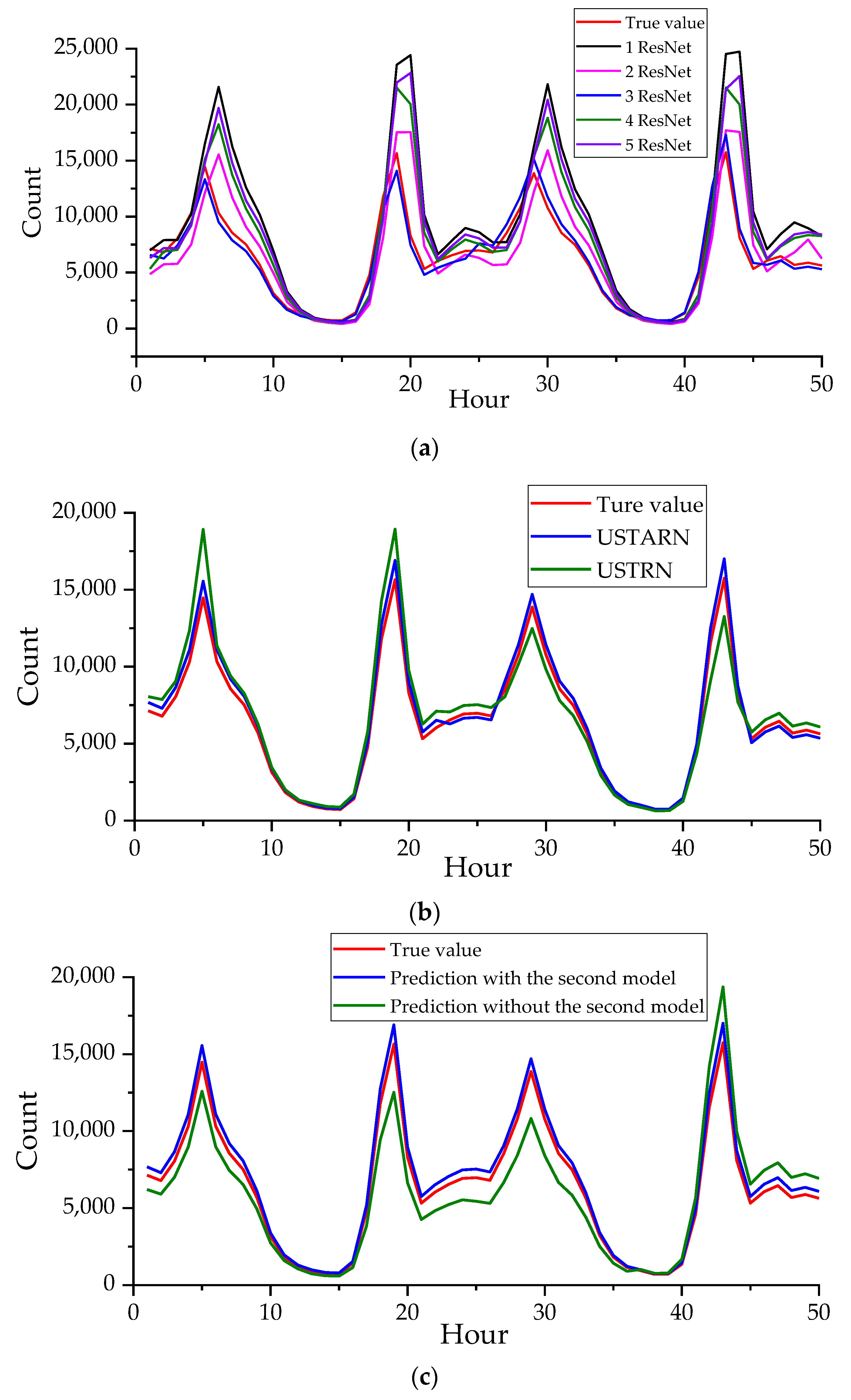
It can be seen from Table 2 that USTARN with a three-layer residual network achieved the best performance. Figure 13 shows the fitting curve between the predicted value and the real value of the bicycle-sharing demand in region 118 of the three experiments on 13 and 14 April 2021. It can be seen from Figure 13a that the prediction accuracy of the network in experiment A initially increased with the increase in the depth of the model, but when it exceeded four layers, the predicted accuracy of the network began to decline, and finally, the performance of the three-layer residual network was the best. This may be because the training difficulty increases when the depth is too deep, which affects the overall accuracy of the model. It is concluded from experiment A that USTARN has the highest accuracy when choosing a three-layer residual network.
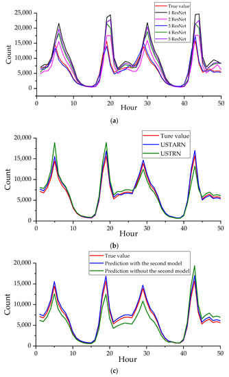
Figure 13.
Comparison of fitting curves of internal experiments of USTARN prediction model in area 118 on 13 and 14 April 2021. (a) Comparison between fitting curve and real value of five network depths in experiment A. (b) Whether the fitting curve of attention mechanism is included in experiment B is compared with the real value. (c) Whether the fitting curve of the second model is included in experiment C and compared with the real value.
It can be seen from Figure 13b that experiment B verifies that the overall prediction accuracy of the model is higher when the three-layer residual network is combined with the attention mechanism to predict the bicycle-sharing demand.
It can be seen from Figure 13c that experiment C proves that the prediction accuracy of USTARN is higher than that modeled without a second model.
To sum up, the best structure of the USTARN model is to include the second prediction model and use the three-layer residual network combined with the attention mechanism. Figure 14 shows the complete test set fitting curve of USTARN. The abscissa is the hour, and the ordinate is the bicycle-sharing demand in the region. The orange broken line is the predicted value of a region, and the blue solid line is the real value of a region. Through the comparison, we can see that the line trend is basically the same, the coincidence degree is high, and the prediction accuracy of the model is high.
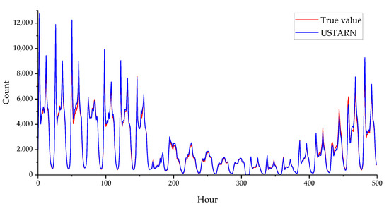
Figure 14.
Fitting curve of test set in area 118.
- (2)
- Baseline experiments
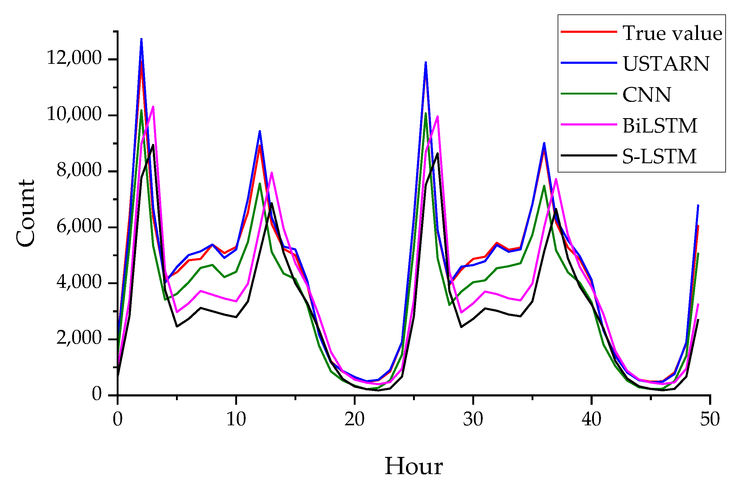
Figure 15 shows the fitting curve between the three basic models and the prediction results of USTARN in area 118 on 13 and 14 April 2021. Meanwhile, Table 3 shows the error values of the three basic models and USTARN. It can be seen from Table 3 and Figure 15 that in the experiment of hourly demand with a step size of 1 in the future, the prediction error of USTARN constructed in this article is the smallest, and the fitting degree is the best. Meanwhile, the USTARN model is superior to the other three models in prediction accuracy. USTARN not only inherits the advantages of the ordinary residual network model, but it also integrates the space-time dimension and other urban factors for prediction, which can further improve the prediction accuracy and make the calculation simpler and more accurate.

Figure 15.
Comparison of fitting curves of four models.
Table 3.
Comparison of MAPE.
5. Discussion
According to the research results, the USTARN demand forecasting method is successfully applied to predict the demand for shared bicycles in all regions of the urban bicycle-sharing system in a certain period of time. In addition, our study is the first to incorporate COVID-19 pandemic elements and analyze its impact on the urban bicycle-sharing systems.
Consistent with the previous results [5], we found that the demand for the bicycle-sharing system shows an obvious temporal regularity. The demand near the residential areas is large in the morning peak period, and the demand near the commercial and industrial land is large in the evening peak period, and there is a significant difference between working days and non-working days. It is found that the demand hot spots in the morning peak period are mainly in the residential areas and the surrounding transportation hubs, and in the evening peak period, they are concentrated in the commercial and industrial land areas, which also corroborates the research of Refs [6,7,12]. In addition, we also found that during COVID-19, the link between the rail transit hubs and the shared bicycles was stronger than that between the buses and shared bicycles, which was also consistent with the findings of Ref. [37].
The degree of infrastructure improvement of the urban shared transportation system is also an important factor affecting its development. By locating the starting and ending points of the morning and evening peak hours, we found that the cycling activities in administrative areas with a complete infrastructure of the shared system are 10 times higher or more than those in other areas. This finding also supports the conclusion in Ref. [38] that the main areas of transportation social exclusion are system infrastructure and operation.
During the global COVID-19 period, we found an interesting phenomenon. When the viral spread in a city leads to a surge in bicycle-sharing demand, and the surge in the number of new confirmed daily patients per 10 people reaches a peak, this may be due to government cutting public services to prevent viral spread. At this time, it is generally believed that the travel mode of shared bicycles presents a lower risk of infection than the travel mode of public transportation, such as the bus and the subway, and this result is a further development of the research in Ref. [14].
Urban shared transportation systems include not only shared bicycles but also shared cars and e-scooters. Due to the particularity of the system, its management has been a hot topic of research. Before the pandemic, Yang et al. [39] designed, for the first time, a shared bicycle prediction system based on hourly granularity with an accuracy of 85% to promote the shared transportation system rebalancing algorithm. Katarzynaturoń et al. [40] put forward suggestions to eliminate social and environmental problems in the development of shared cars by analyzing the types of social exclusion in transportation. Suggestions on rulemaking for the use of shared e-scooters have also been made [41]. The above are the studies of scholars on different subsystems of the urban shared transport system. Our research results are also consistent with these research conclusions regarding the general direction and bear many similarities. However, due to the difficulty in data collection, more traffic social exclusion factors are not taken into account. In the follow-up study, more factors affecting the development of a shared system can be filled in, and a comprehensive study can be conducted in combination with a variety of shared modes.
6. Conclusions
Urban computing is an emerging research field, which aims at using a variety of different kinds and different dimensions of information generated in cities to study and solve problems that exist in urban development, such as traffic congestion, energy consumption, environmental pollution and so on.
An extremely significant contribution lies in the findings concerning exploring the demand patterns of shared transportation systems during the epidemic period. The spatial-temporal attention residual network demand prediction model (USTARN) based on the bicycle-sharing demand during COVID-19 constructed in this paper fully considers the spatial and temporal characteristics of the bicycle-sharing demand and their dependence. The MAPE of USTARN demand prediction results is 7.89%, which is 15.69%, 15.34% and 7.72% lower than the traditional S-LSTM, BiLSTM and CNN prediction models, respectively. USTARN obtains the highest prediction accuracy of the four models and is superior to the other traditional models in terms of calculation simplicity and accuracy. USTRAN improves the precision and accuracy of the demand forecast of the bicycle-sharing system.
The difference between our study and the previous demand prediction of shared transportation is that the epidemic element is added, and for the first time, the residual model combined with the attention mechanism at different periods and regions is used to predict the demand for shared bicycles. USTARN improves the precision and accuracy of the demand prediction of the shared bicycle system. The data of travel demand of shared bicycles, geographic information data, climate data, epidemic data and time data generated in the city are used to predict the travel demand of shared bicycles in batches by regions and time segments, and the forecast results of travel demand of all regions in a certain period in the future are output. In the current visual analysis, we found that the use of shared bicycles was significantly correlated with land use, the clustering degree of bus hubs, public transport services, weather conditions, holidays and the severity of the epidemic. The demand for shared bicycles increased to varying degrees when the scale of public transport services was reduced and when the COVID-19 pandemic occurred. Cycling demand also showed a significant correlation with temperature. The research found that 23 °C was the best temperature for cycling, and the demand decreased significantly when the minimum temperature was lower than 9 °C and higher than 3 °C. Therefore, we put forward the following suggestions on the operation and resource allocation of the bicycle-sharing system:
(1) The operation scale can be appropriately scaled down, and old bicycles can be recycled in winter to reduce the waste of resources. And the operation department can increase the supply of shared bicycles at parking points in residential areas and the surrounding bus hubs during the morning peak period and accelerate the construction of shared traffic infrastructure in the surrounding areas to reasonably allocate shared traffic resources.
(2) During the pandemic period, urban managers should strengthen the management, maintenance, disinfection and sterilization of the shared transportation system and strengthen the cycling constraints in the urban road network to ensure the safety and reliability of cycling.
In summary, USTARN added the epidemic elements compared with the demand prediction of the shared transportation system at present and, for the first time, used the residual model combined with the attention mechanism at different periods and regions to forecast the demand for shared bicycles. USTARN improved the shared-cycling system demand forecast precision and accuracy using the city of shared-bicycle travel demand data, geographic information data, climate data, epidemic data and time data to predict the shared-bicycle travel demand forecast period of time in the batch areas and the output travel demand forecast in all areas of the future at a certain period of time. It achieved the expected goal, and it can be applied to urban problems related to the demand prediction for shared bicycles, which has universal applicability. This study drew lessons from the research achievements, which exist at present, establishing a new bicycle-sharing demand forecasting model (USTARN) that filled the urban shared traffic system in the law of development of blank COVID-19 pandemic period. It achieved a high accuracy of prediction of shared-cycling demand, and the universal model was set up at the same time to also consider the development of the spread of the epidemic. We provided a theoretical basis for governments and operators to further formulate development plans and management regulations for shared transportation systems during the duration of public health events. In fact, due to the outbreak and instability of the epidemic and the limited amount of epidemic data obtained, the prediction accuracy of the model still needs to be improved. In addition, due to the complex and diverse socioeconomic factors and traffic social exclusion that restrict the development of the urban shared transportation system [40,41], more influencing factors can be added in future works to improve the prediction ability of the model. Nevertheless, the general regularities and model methods obtained in this study can still be used as reference by similar studies.
Author Contributions
Conceptualization, Y.C. and Y.W.; methodology, Y.C. and Y.W.; software, Y.W.; investigation, Y.W.; validation, Y.W.; visualization, Y.C. and Y.W.; writing—original draft preparation, Y.C. and Y.W. All authors have read and agreed to the published version of the manuscript.
Funding
This research was supported by the Scientific Research Funding Project of Liaoning Provincial Education Department in 2020 (grant No. JDL2020017), the Research Project on Economic and Social Development of Liaoning Province in 2022 by the Liaoning Provincial Federation Social Science Circles (grant No. 2022lslybkt-022), the 2021 and 2022 Project of Dalian Academy of Social Sciences (grant No. 2021dlsky050, 2022dlsky078), the Education Quality Improvement Project for Post-graduate of Dalian Jiaotong University and the Teaching Reform Research Project for Undergraduate of Dalian Jiaotong University.
Institutional Review Board Statement
Not applicable.
Informed Consent Statement
Not applicable.
Data Availability Statement
Not applicable.
Acknowledgments
The authors would like to thank the historical order data samples of shared bicycles provided by the data open platform of the Shenzhen municipal government, the historical data of COVID-19 provided by the Shenzhen CDC and the historical information data of weather conditions in Shenzhen provided by the Shenzhen Meteorological Bureau as the experimental materials of this study. We are also grateful to the editors and anonymous reviewers for their suggestions and comments.
Conflicts of Interest
The authors declare no conflict of interest.
Abbreviations
The following abbreviations are used in this manuscript:
| COVID-19 | Corona Virus Disease 2019 |
| DBSCAN | Density-based spatial clustering of applications with noise |
| GPS | Global Positioning System |
| CDC | Centers for Disease Control |
| MAPE | Mean Absolute Percentage Error |
References
- Zhang, J.P.; Wang, F.Y.; Wang, K.F.; Lin, W.H.; Xu, X.; Chen, C. Data-Driven Intelligent Transportation Systems: A Survey. IEEE Trans. Intell. Transp. Syst. 2011, 12, 1624–1639. [Google Scholar] [CrossRef]
- Dai, G.N.; Hu, X.Y.; Ge, Y.M.; Ning, Z.Q.; Liu, Y.B. Attention based simplified deep residual network for citywide crowd flows prediction. Front. Comput. Sci. 2021, 15, 152317. [Google Scholar] [CrossRef]
- Hui, Y.; Liao, J.M.; Tang, L.; Xie, Y.K.; Li, J. Travel behavior and preference using bike sharing during the pandemic. Urban Transp. China 2020, 18, 100–109. [Google Scholar] [CrossRef]
- Beijing Comprehensive Transportation Development Research Institute of Beijing Jiaotong University. Beijing Transportation Blue Book: Beijing Transportation Development Report (2021); Social Science Literature Press: Beijing, China, 2022; ISBN 9787520195560. [Google Scholar]
- Fu, X.M.; Juan, Z.C. Unraveling mobility pattern of dockless bike-sharing use in Shanghai. J. Transp. Syst. Eng. Inf. Technol. 2020, 20, 219–226. [Google Scholar] [CrossRef]
- Zhao, X.F.; Hu, C.Y.; Liu, Z.; Meng, Y.Y. Weighted dynamic time warping for grid-based travel-demand-pattern clustering: Case study of Beijing bicycle-sharing system. ISPRS Int. J. Geo-Inf. 2019, 8, 281. [Google Scholar] [CrossRef] [Green Version]
- Gao, Y.; Song, C.; Shu, H.; Pei, T. Spatial-temporal characteristics of source and sink points of Mobikes in Beijing and its scheduling strategy. J. Geo-Inf. Sci. 2018, 20, 1123–1138. [Google Scholar] [CrossRef]
- Du, Y.C.; Deng, F.W.; Liao, F.X. A model framework for discovering the spatio-temporal usage patterns of public free-floating bike-sharing system. Transp. Res. Part C 2019, 103, 39–55. [Google Scholar] [CrossRef]
- Zhang, Y.P.; Lin, D.; Mi, Z.F. Electric fence planning for dockless bike- sharing services. J. Clean. Prod. 2019, 206, 383–393. [Google Scholar] [CrossRef]
- Yu, J.J.; Ji, Y.J.; Yi, C.Y.; Liu, Y. Estimating model for urban carrying capacity on bike- sharing. J. Cent. South Univ. 2021, 28, 1775–1785. [Google Scholar] [CrossRef]
- Hua, M.Z.; Chen, X.W.; Zheng, S.J.; Chen, L.; Chen, J.X. Estimating the parking demand of free- floating bike sharing: A journeydata-based study of Nanjing, China. J. Clean. Prod. 2020, 244, 118764. [Google Scholar] [CrossRef]
- Wang, Y.C.; Douglas, M.; Hazen, B. Diffusion of public bicycle systems: Investigating influences of users perceived risk and switching intention. Transp. Res. Part A 2021, 143, 1–13. [Google Scholar] [CrossRef]
- Sun, Q.P.; Zeng, K.B.; Zhang, K.Q.; Yang, Y.C.; Zhang, S.X. Spatiotemporal travel patterns and demand prediction of shared bikes in Beijing. J. Transp. Syst. Eng. Inf. Technol. 2022, 22, 332–338. [Google Scholar] [CrossRef]
- Zhang, Y.C.; Fricker, J.D. Quantifying the impact of COVID-19 on non-motorized transportation: A Bayesian structural time series model. Transp. Policy 2021, 103, 11–20. [Google Scholar] [CrossRef]
- El-Assi, W.; Mahmoud, M.S.; Habib, K.N. Effects of built environment and weather on bike sharing demand: A station level analysis of commercial bike sharing in Toronto. Transportation 2017, 44, 589–613. [Google Scholar] [CrossRef]
- Zhang, Y.; Thomas, T.; Brussel, M.; Maarseveen, M.V. Exploring the impact of built environment factors on the use of public bikes at bike stations: Case study in Zhongshan, China. J. Transp. Geogr. 2017, 58, 59–70. [Google Scholar] [CrossRef]
- Guidon, S.; Becker, H.; Dediu, H.; Axhausen, K.W. Electric Bicycle-Sharing: A New Competitor in the Urban Transportation Market? An Empirical Analysis of Transaction Data. Transp. Res. Rec. 2019, 2673, 1–12. [Google Scholar] [CrossRef]
- Kapuku, C.; Kho, S.Y.; Kim, D.K.; Cho, S.H. Modeling the competitiveness of a bike- sharing system using bicycle GPS and transit smartcard data. Transp. Lett. Int. J. Transp. Res. 2020, 1, 347–351. [Google Scholar] [CrossRef]
- Yang, Z.J.; Ma, Q.Y. Evolutionary game analysis of shared bike cyclists’ opportunistic behaviour. J. Ind. Eng. 2020, 34, 104–111. [Google Scholar] [CrossRef]
- Feng, S.J.; Chen, H.; Du, C.; Li, J. A hierarchical demand prediction method with station clustering for bike sharing system. In Proceedings of the 2018 IEEE Third International Conference on Data Science in Cyberspace (DSC), Guangzhou, China, 18–21 June 2018; pp. 829–836. [Google Scholar]
- Peng, Y.; Zhang, W.; Wan, F. Demand prediction for station clusters in bike sharing system. Comput. Appl. Softw. 2021, 38, 92–98, 110. [Google Scholar] [CrossRef]
- Huang, F.H.; Qiao, S.J.; Peng, J.; Guo, B. A Bimodal Gaussian Inhomogeneous Poisson Algorithm for Bike Number Prediction in a Bike-Sharing System. IEEE Trans. Intell. Transp. Syst. 2019, 20, 1–10. [Google Scholar] [CrossRef]
- Li, X.H.; Zhang, X.Y.; Cheng, C.; Yang, C.; Wang, W. Dynamic repositioning model for free-floating bike-sharing system considering shifting demand. J. Transp. Syst. Eng. Inf. Technol. 2020, 20, 182–189. [Google Scholar] [CrossRef]
- Qiao, S.J.; Han, N.; Yue, K.; Yi, Y.G.; Huang, F.L.; Yuan, C.A.; Ding, P.; Gutierrez, L.A. Shared-bike demand prediction model based on station clustering. J. Softw. 2022, 33, 1451–1476. [Google Scholar] [CrossRef]
- Ashqar, H.I.; Elhenawy, M.; Almannaa, M.H.; Ghanem, A.; Rakha, H.A.; House, L. Modeling bike availability in a bike-sharing system using machine learning. In Proceedings of the 2017 5th IEEE International Conference on Models and Technologies for Intelligent Transportation Systems (MT-ITS), Naples, Italy, 26–28 June 2017; pp. 374–378. [Google Scholar]
- Xu, C.C.; Ji, J.Y.; Liu, P. The station-free sharing bike demand forecasting with a deep learning approach and large-scale datasets. Transp. Res. Part C 2018, 95, 47–60. [Google Scholar] [CrossRef]
- Jiang, X.; Bai, L.B.; Lou, X.Y.; Li, M.; Liu, H. Usage patterns identification and flow prediction of bike-sharing system based on multiscale spatiotemporal clustering. J. Geo-Inf. Sci. 2022, 24, 1047–1060. [Google Scholar] [CrossRef]
- Julia, P.; Przemyslaw, A.G.; Ryota, K.; Carlos, C.; Philippe, C.-M.; Karl, A. Predicting the success of online petitions leveraging multidimensional time-series. In Proceedings of the WWW ’17: Proceedings of the 26th International Conference on World Wide Web, Perth, Australia, 3–7 April 2017; Volume 5, pp. 755–764. [Google Scholar] [CrossRef] [Green Version]
- Qiao, S.J.; Han, N.; Wang, J.F.; Li, R.H.; Gutierrez, L.A.; Wu, X.D. Predicting Long-Term Trajectories of Connected Vehicles via the Prefix-Projection Technique. IEEE Trans. Intell. Transp. Syst. 2018, 19, 2305–2315. [Google Scholar] [CrossRef]
- Chai, D.; Wang, L.Y.; Yang, Q. Bike flow prediction with multi-graph convolutional networks. In Proceedings of the 26th ACM SIGSPATIAL International Conference on Advances in Geographic Information Systems—SIGSPATIAL ’18, Kunming, China, 6 November 2018; pp. 397–400. [Google Scholar]
- Zhang, J.B.; Zheng, Y.; Qi, D.K. Deep Spatio-Temporal Residual Networks for Citywide Crowd Flows Prediction. In Proceedings of the Thirty-First AAAI Conference on Artificial Intelligence (AAAI-17), San Francisco, CA, USA, 4–9 February 2017; pp. 1655–1661. [Google Scholar]
- Guo, S.N.; Lin, Y.F.; Feng, N.; Song, C.; Wan, H.Y. Attention Based Spatial-Temporal Graph Convolutional Networks for Traffic Flow Forecasting. In Proceedings of the AAAI Conference on Artificial Intelligence 2019, Honolulu, HI, USA, 27 January–1 February 2019; pp. 922–929. [Google Scholar]
- Liu, Y.C.; Li, Z.P.; Lv, C.P.; Zhang, T.; Liu, Y. Network-wide traffic flow prediction research based on DTW algorithm spatial-temporal graph convolution. J. Transp. Syst. Eng. Inf. Technol. 2022, 22, 1–17. Available online: https://kns.cnki.net/kcms/detail/11.4520.U.20220412.1314.010.html (accessed on 13 April 2022).
- Zeng, J.C.; Shao, M.H.; Sun, L.J.; Lu, C. Traffic prediction and congestion control based on directed graph convolution neural network. China J. Highw. Transp. 2021, 34, 239–248. [Google Scholar] [CrossRef]
- Kingma, D.; Ba, J. Adam: A method for stochastic optimization. In Proceedings of the 3rd International Conference on Learning Representations (ICLR 2015), San Diego, CA, USA, 7–9 May 2015; pp. 1–15. [Google Scholar]
- Lin, L.; He, Z.B.; Peeta, S. Predicting station-level hourly demand in a large-scale bike-sharing network: A graph convolutional neural network approach. Transp. Res. Part C 2018, 97, 258–276. [Google Scholar] [CrossRef] [Green Version]
- Jaber, A.; Baker, L.A.; Csonka, B. The Influence of Public Transportation Stops on Bike-Sharing Destination Trips: Spatial Analysis of Budapest City. Future Transp. 2022, 2, 688–697. [Google Scholar] [CrossRef]
- Turoń, K. Complaints Analysis as an Opportunity to Counteract Social Transport Exclusion in Shared Mobility Systems. Smart Cities 2022, 5, 875–888. [Google Scholar] [CrossRef]
- Yang, Z.D.; Hu, J.; Shu, Y.C.; Cheng, P.; Chen, J.M.; Moscibroda, T. Mobility Modeling and Prediction in Bike-Sharing Systems. In Proceedings of the Mobile Systems, Applications, and Services 2016, Singapore, 25–30 June 2016; pp. 165–178. [Google Scholar]
- Turoń, K.; Czech, P. The Concept of Rules and Recommendations for Riding Shared and Private E-Scooters in the Road Network in the Light of Global Problems. Sci. Tech. Conf. Transp. Syst. Theory Pract. 2019, 1083, 275–284. [Google Scholar] [CrossRef]
- Turoń, K. Soical Barriers and Transportation Social Exclusion Issues in Creating Sustainable Car-Sharing Syetems. Entrep. Sustain. Issues 2021, 9, 10–22. [Google Scholar] [CrossRef]


Publisher’s Note: MDPI stays neutral with regard to jurisdictional claims in published maps and institutional affiliations. |
© 2022 by the authors. Licensee MDPI, Basel, Switzerland. This article is an open access article distributed under the terms and conditions of the Creative Commons Attribution (CC BY) license (https://creativecommons.org/licenses/by/4.0/).