
Quantifying Subnational Economic Complexity: Evidence from Romania


Abstract
:1. Introduction
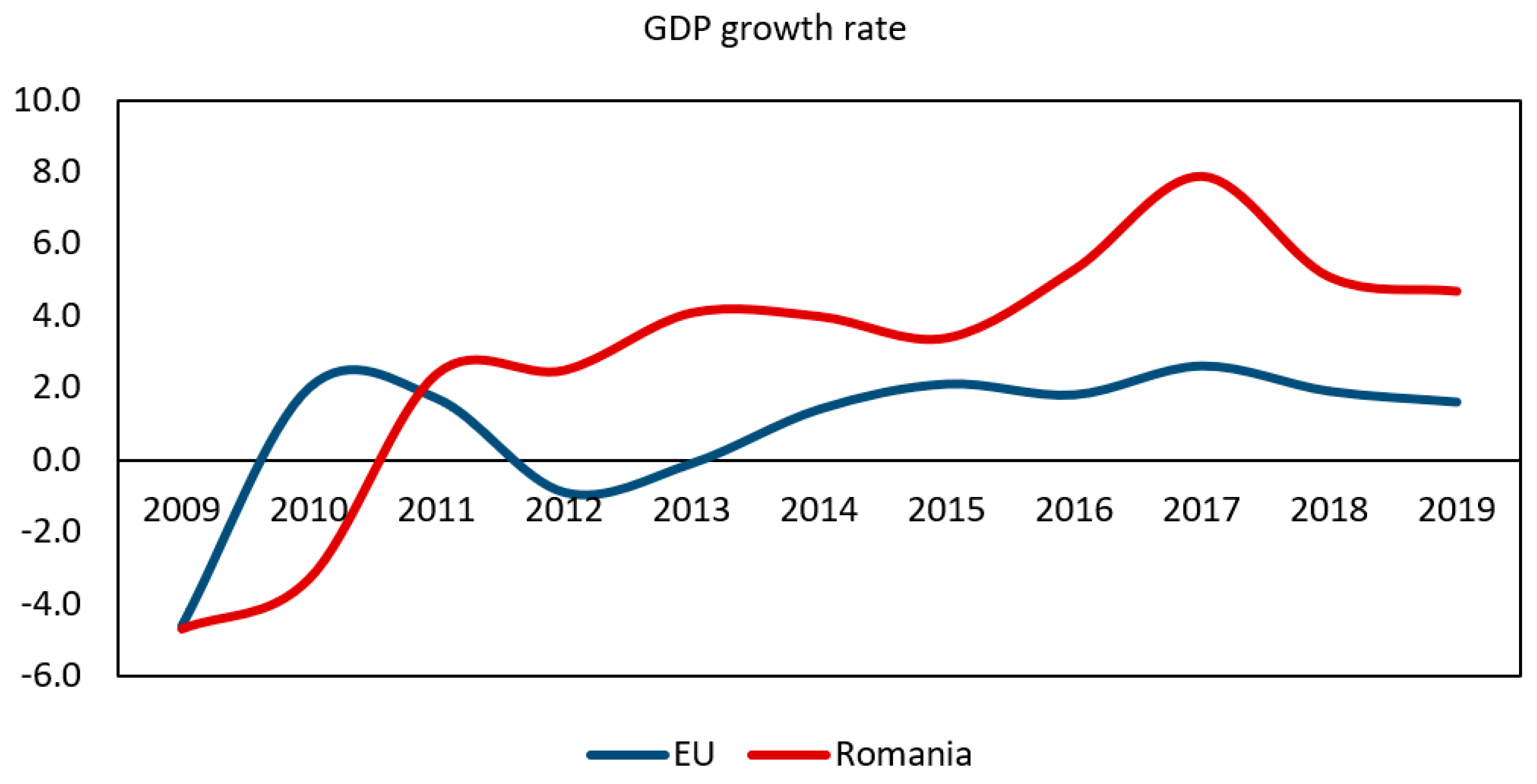
2. Study Area
3. Data and Method
3.1. Data Collection
3.2. Methods for Analyzing the Economic Complexity Index
3.2.1. Defining the Revealed Comparative Advantage of Counties
3.2.2. Applying the Method of Reflection (MR) Technique
3.2.3. Calculation of the Economic Complexity Index
3.2.4. Applying the Multivariate Regression Analysis
4. Results and Discussion
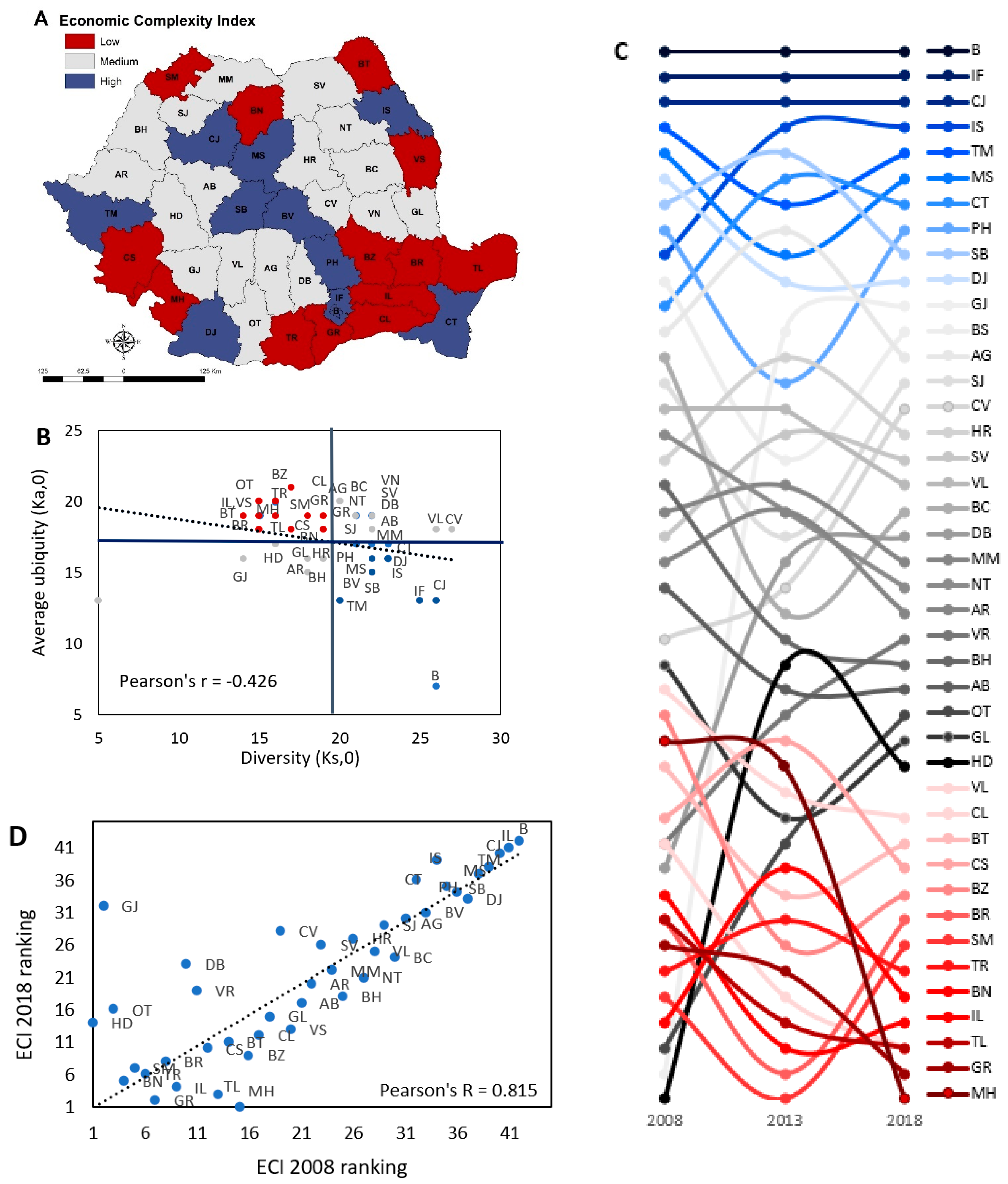
4.1. Measuring Subnational Economic Complexity (ECI)
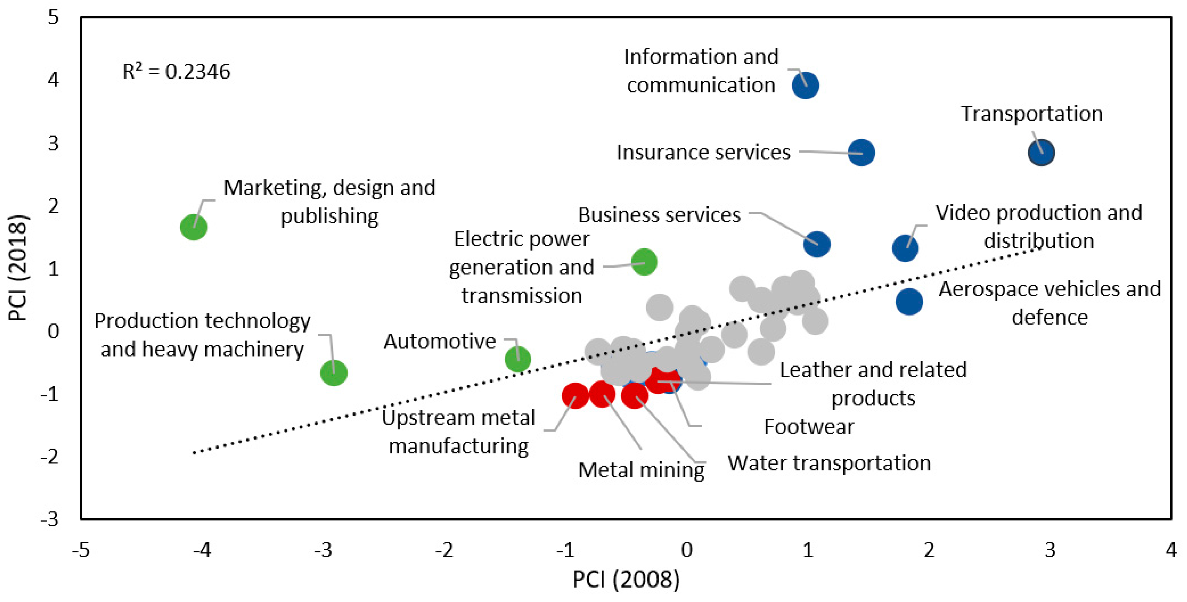
4.2. Measuring Product Complexity (PCI)
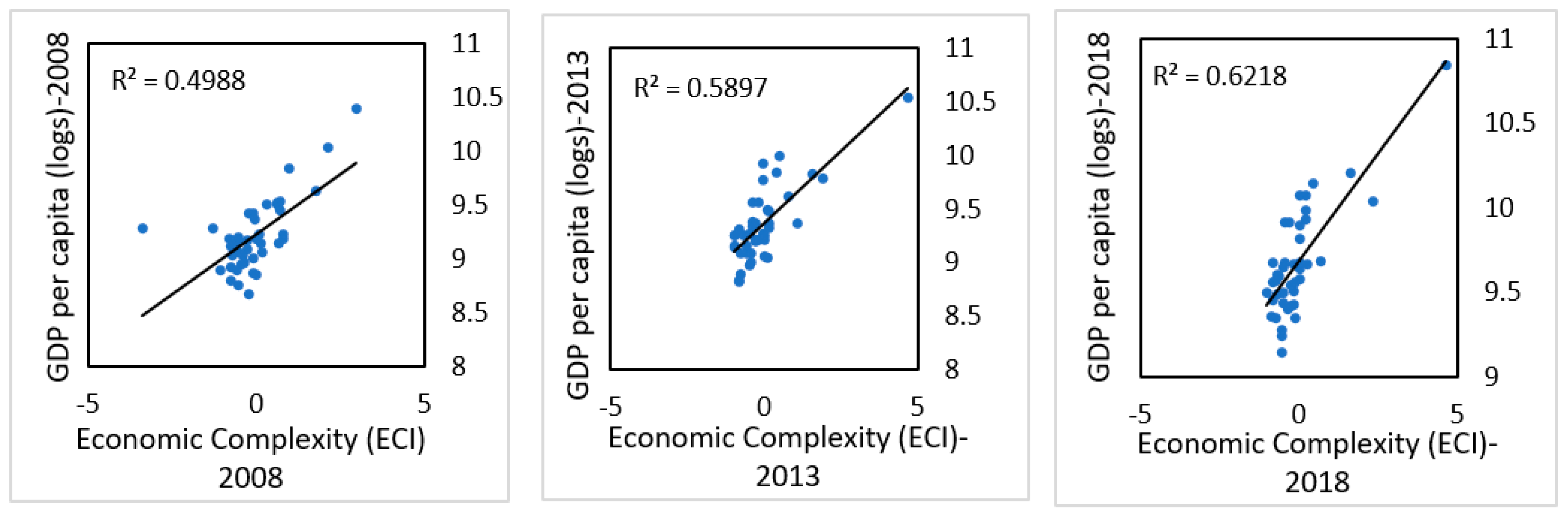
4.3. The Relation between Economic Complexity and Income Inequality
5. Conclusions
Author Contributions
Funding
Data Availability Statement
Conflicts of Interest
Appendix A

| ID | County | Abbrev. | ID | County | Abbrev. | ID | County | Abbrev. |
|---|---|---|---|---|---|---|---|---|
| 1 | Alba | AB | 15 | Constanta | CT | 29 | Mures | MS |
| 2 | Arges | AG | 16 | Covasna | CV | 30 | Neamt | NT |
| 3 | Arad | AR | 17 | Dâmbovita | DB | 31 | Olt | OT |
| 4 | Bucuresti | B | 18 | Dolj | DJ | 32 | Prahova | PH |
| 5 | Bacău | BC | 19 | Gorj | GJ | 33 | Sibiu | SB |
| 6 | Bihor | BH | 20 | Galati | GL | 34 | Sălaj | SJ |
| 7 | Bistrita-Năsăud | BN | 21 | Giurgiu | GR | 35 | Satu Mare | SM |
| 8 | Brăila | BR | 22 | Hunedoara | HD | 36 | Suceava | SV |
| 9 | Botosani | BT | 23 | Harghita | HR | 37 | Tulcea | TL |
| 10 | Brasov | BV | 24 | Ilfov | IF | 38 | Timis | TM |
| 11 | Buzău | BZ | 25 | Ialomita | IL | 39 | Teleorman | TR |
| 12 | Cluj | CJ | 26 | Iasi | IS | 40 | Vâlcea | VL |
| 13 | Călărasi | CL | 27 | Mehedinti | MH | 41 | Vrancea | VN |
| 14 | Caras-Severin | CS | 28 | Maramures | MM | 42 | Vaslui | VS |
| Global Industries Clusters | |||
|---|---|---|---|
| 1 | Aerospace Vehicles and Defense | 27 | Leather and Related Products |
| 2 | Agricultural Inputs and Services | 28 | Lighting and Electrical Equipment |
| 3 | Apparel | 29 | Livestock Processing |
| 4 | Appliances | 30 | Marketing, Design, and Publishing |
| 5 | Automotive | 31 | Medical Devices |
| 6 | Biopharmaceuticals | 32 | Metal Mining |
| 7 | Business Services | 33 | Metalworking Technology |
| 8 | Coal Mining | 34 | Music and Sound Recording |
| 9 | Communications Equipment and Services | 35 | Non-metal mining |
| 10 | Construction Products and Services | 36 | Oil and Gas Production and Transportation |
| 11 | Distribution and Electronic Commerce | 37 | Paper and Packaging |
| 12 | Downstream Chemical Products | 38 | Performing Arts |
| 13 | Downstream Metal Products | 39 | Plastics |
| 14 | Education and Knowledge Creation | 40 | Printing Services |
| 15 | Electric Power Generation and Transmission | 41 | Production Technology and Heavy Machinery |
| 16 | Environmental Services | 42 | Recreational and Small Electric Goods |
| 17 | Financial Services | 43 | Textile Manufacturing |
| 18 | Fishing and Fishing Products | 44 | Tobacco |
| 19 | Food Processing and Manufacturing | 45 | Transportation and Logistics |
| 20 | Footwear | 46 | Upstream Chemical Products |
| 21 | Forestry | 47 | Upstream Metal Manufacturing |
| 22 | Furniture | 48 | Video Production and Distribution |
| 23 | Hospitality and Tourism | 49 | Vulcanized and Fired Materials |
| 24 | Information Technology and Analytical Instruments | 50 | Water Transportation |
| 25 | Insurance Services | 51 | Wood Products |
| 26 | Jewelry and Precious Metals | ||
| Local industries clusters | |||
| 1 | Agriculture, Forestry and Fishing | 10 | Financial and Insurance Activities |
| 2 | Manufacturing | 11 | Real Estate Activities |
| 3 | Electricity, Gas, Steam and Air Conditioning Supply | 12 | Professional, Scientific and Technical Activities |
| 4 | Water Supply; Sewerage, Waste Management and Remediation Activities | 13 | Administrative and Support Service Activities |
| 5 | Construction | 14 | Public Administration and Defense; Compulsory Social Security |
| 6 | Wholesale and Retail Trade; Repair of Motor Vehicles and Motorcycles | 15 | Education |
| 7 | Transportation and Storage | 16 | Human Health and Social Work Activities |
| 8 | Accommodation and Food Service Activities | 17 | Arts, Entertainment and Recreation |
| 9 | Information and Communication | ||

References
- Gao, J.; Zhou, T. Quantifying China’s regional economic complexity. Physica A 2018, 492, 1591–1603. [Google Scholar] [CrossRef]
- Benedek, J.; Temerdek-Ivan, K.; Török, I.; Temerdek, A.; Holobâcă, I.H. Indicator based assessment of local and regional progress towards the Sustainable Development Goals (SDGs): An integrated approach from Romania. Sustain. Dev. 2021, 29, 860–875. [Google Scholar] [CrossRef]
- Hidalgo, C.A.; Hausmann, R. The building blocks of economic complexity. Proc. Natl. Acad. Sci. USA 2009, 106, 10570–10575. [Google Scholar] [CrossRef] [PubMed]
- Andersen, T.B.; Dalgaard, C. Flows of people, flows of ideas, and the inequality of nations. J. Econ. Growth 2011, 16, 1–32. [Google Scholar] [CrossRef]
- Hartmann, D. Economic Complexity and Human Development: How Economic Diversification and Social Networks Affect Human Agency and Welfare, 1st ed.; Routledge: New York, NY, USA, 2014; pp. 63–91. [Google Scholar]
- Hausmann, R.; Hidalgo, C.A. The network structure of economic output. J. Econ. Growth 2011, 16, 309–342. [Google Scholar] [CrossRef]
- Balland, P.A.; Rigby, D. The Geography of Complex Knowledge. J. Econ. Geogr. 2017, 93, 1–23. [Google Scholar] [CrossRef]
- Hirschman, A. The Strategy of Economic Development, 1st ed.; Yale University Press: New Haven, UK, 1958; pp. 25–72. [Google Scholar]
- Kuznets, S. Modern Economic Growth, 1st ed.; Yale University Press: New Haven, UK, 1966; pp. 1–89. [Google Scholar]
- Lewis, A. The Theory of Economic Growth, 1st ed.; Routledge: New York, NY, USA, 1955; pp. 420–436. [Google Scholar]
- Hidalgo, C. Economic complexity theory and applications. Nat. Rev. Phys. 2021, 3, 92–113. [Google Scholar] [CrossRef]
- Felipe, J.; Kumar, U.; Abdon, A.; Bacate, M. Product complexity and economic development. Struct. Change Econ. D 2012, 23, 36–68. [Google Scholar] [CrossRef]
- Britto, G.; Romero, J.; Freitas, E.; Coelho, C. The great divide: Economic complexity and development paths in Brazil and the Republic of Korea. CEPAL Rev. 2019, 127, 191–213. [Google Scholar] [CrossRef]
- Fukuyama, F. Trust: Human Nature and the Reconstitution of Social Order, 1st ed.; Free Press: New York, NY, USA, 1996; pp. 3–49. [Google Scholar]
- Hidalgo, C. Why Information Grows: The Evolution of Order, from Atoms to Economies, 1st ed.; Basic Books: New York, NY, USA, 2015; pp. 1–258. [Google Scholar]
- Hausmann, R.; Hidalgo, C.A.; Bustos, S.; Coscia, M.; Simoes, A.; Chung, S.; Jimenez, J.; Simoes, A.; Yildirim, M.A. The Atlas of Economic Complexity: Mapping Paths to Prosperity, 1st ed.; MIT Press: Cambridge, MA, USA; London, UK, 2011; pp. 1–71. [Google Scholar]
- Panzera, D.; Postiglione, P. The impact of regional inequality on economic growth: A spatial econometric approach. Reg. Stud. 2022, 56, 687–702. [Google Scholar] [CrossRef]
- Daboin, C.; Escobari, M.; Hernández, G.; Morales-Arilla, J. Economic Complexity and Technological Relatedness: Findings for American Cities. 2019. Available online: https://www.semanticscholar.org/paper/D-raft-as-of-M-ay-16-%2C-2019-Economic-Complexity-and-Daboin-Escobari/2ca55ffe850598548c9ec3fa913f4c100949d194#citing-papers (accessed on 5 April 2022).
- Gómez-Zaldívar, M.; Llanos-Guerrero, A. On the synchronization of the business cycles of Mexican states and its relationship to their economic complexity, 2000–2014. Growth Chang. 2021, 52, 1576–1592. [Google Scholar] [CrossRef]
- Ferraz, D.; Falguera, F.P.S.; Mariano, E.B.; Hartmann, D. Linking Economic Complexity, Diversification, and Industrial Policy with Sustainable Development: A Structured Literature Review. Sustainability 2021, 13, 1265. [Google Scholar] [CrossRef]
- Hartmann, D.; Guevara, M.R.; Jara-Figueroa, C.; Aristarab, M.; Hidalgo, C.A. Linking Economic Complexity, Institutions, and Income Inequality. World Dev. 2017, 93, 75–93. [Google Scholar] [CrossRef]
- Hartmann, D.; Jara-Figueroa, C.; Guevara, M.; Simoes, A.; Hidalgo, C.A. The structural constraints of income inequality in Latin America. Integr. Trade J. 2017, 40, 70–85. [Google Scholar] [CrossRef]
- Kangkook, L.; Trung, V. Economic Complexity, Human Capital and Income Inequality: A Cross-Country Analysis. MPRA Paper No 94918. 2019. Available online: https://mpra.ub.uni-muenchen.de/94918/ (accessed on 17 July 2021).
- Roos, G. Technology-Driven Productivity Improvements and the Future of Work: Emerging Research and Opportunities, 1st ed.; IGI Global: Hershey, PA, USA, 2017; pp. 150–167. [Google Scholar]
- Basile, R.; Cicerone, G.; Iapadre, L. Economic Complexity and Regional Labor Productivity Distribution: Evidence from Italy. 2019. Available online: https://siecon3-607788.c.cdn77.org/sites/siecon.org/files/media_wysiwyg/8-basile-cicerone-iapadre.pdf (accessed on 19 August 2021).
- Sweet, C.; Eterovic, D. Do patent rights matter? 40 years of innovation, complexity and productivity. World Dev. 2019, 115, 78–93. [Google Scholar] [CrossRef]
- Javorcik, B.; Lo Turco, A.; Maggioni, D. New and improved: Does FDI boost production complexity in host countries? Econ. J. 2017, 128, 2507–2537. [Google Scholar] [CrossRef]
- Khan, H.; Khan, U.; Khan, M.A. Causal nexus between economic complexity and FDI: Empirical evidence from time series analysis. Chin. Econ. 2020, 53, 374–394. [Google Scholar] [CrossRef]
- Can, M.; Gozgor, G. The impact of economic complexity on carbon emissions: Evidence from France. Environ. Sci. Pollut. Res. 2017, 24, 16364–16370. [Google Scholar] [CrossRef]
- Neagu, O.; Teodoru, M.C. The Relationship between Economic Complexity, Energy Consumption Structure and Greenhouse Gas Emission: Heterogeneous Panel Evidence from the EU Countries. Sustainability 2019, 11, 497. [Google Scholar] [CrossRef]
- Boleti, E.; Garas, A.; Kyriakou, A.; Lapatinas, A. Economic complexity and environmental performance: Evidence from a world sample. Environ. Model. Assess. 2021, 26, 251–270. [Google Scholar] [CrossRef]
- Romero, J.P.; Gramkow, C. Economic complexity and greenhouse gas emissions. World Dev. 2021, 139, 105317. [Google Scholar] [CrossRef]
- Voicu-Dorobantu, R.; Volintiri, C.; Popescu, M.F.; Nerau, F.; Stefan, G. Tackling complexity of the just transition in the EU: Evidence from Romania. Energies 2021, 14, 1509. [Google Scholar] [CrossRef]
- Fritz, B.S.L.; Manduka, R.A. The economic complexity of US metropolitan areas. Reg. Stud. 2021, 55, 1299–1310. [Google Scholar] [CrossRef]
- Chávez, J.C.; Mosqueda, M.T.; Gómez-Zaldívar, M. Economic Complexity and Regional Growth Performance: Evidence from the Mexican Economy. Rev. Reg. Stud. 2017, 47, 201–219. [Google Scholar] [CrossRef]
- Operti, F.G.; Pugliese, E.; Andrade, J.S.; Pietronero, L.; Gabrielli, A. Dynamics in the Fitness-Income plane: Brazilian states vs World countries. PLoS ONE 2019, 14, e0197616. [Google Scholar] [CrossRef] [PubMed]
- Reynolds, C.; Agrawal, M.; Lee, I.; Zhan, C.; Li, J.; Taylor, P.; Mares, T.; Morison, J.; Angelakis, N.; Roos, G. A sub-national economic complexity analysis of Australia’s states and territories. Reg. Stud. 2018, 52, 715–726. [Google Scholar] [CrossRef]
- Balsalobre, P.S.; Verduras, L.C.; Lanchas, D.J. Measuring Subnational Economic Complexity: An Application with Spanish Data; JRC Working Papers on Territorial Modelling and Analysis; European Comission: Seville, Spain, 2019; Volume 5. Available online: https://ec.europa.eu/jrc/sites/default/files/jrc116253.pdf (accessed on 24 June 2021).
- Cicerone, G.; McCann, P.; Venhorst, V.A. Promoting regional growth and innovation: Relatedness, revealed comparative advantage and the product space. J. Econ. Geogr. 2020, 20, 293–316. [Google Scholar] [CrossRef]
- Davies, B.; Maré, D.C. Relatedness, complexity and local growth. Reg. Stud. 2021, 55, 479–494. [Google Scholar] [CrossRef]
- Mealy, P.; Coyle, D. Economic Complexity Analysis; Greater Manchester Independent Prosperity Review; Bennett Institute for Public Policy: Cambridge, UK, 2019; Available online: www.gmprosperityreview.co.uk (accessed on 17 June 2021).
- Milanovic, B. Global Income Inequality by the Numbers: In History and Now-An Overview; Policy Research Working Paper WPS 6259; World Bank: Washington, DC, USA, 2012; Available online: https://openknowledge.worldbank.org/bitstream/handle/10986/12117/wps6259.pdf?sequence=2&isAllowed=y (accessed on 17 October 2021).
- Le Caous, E.; Huarng, F. Economic Complexity and the Mediating Effects of Income Inequality: Reaching Sustainable Development in Developing Countries. Sustainability 2020, 12, 2089. [Google Scholar] [CrossRef]
- Bandeira-Morais, M.; Swart, J.; Jordaan, J.A. Economic complexity and inequality: Does productive structure affect regional wage differentials in Brazil? Sustainability 2021, 13, 1006. [Google Scholar] [CrossRef]
- Pinheiro, F.L.; Balland, P.A.; Boschma, R.; Hartmann, D. The dark side of geography of innovation. Relatedness, complexity and regional inequality in Europe. Pap. Evol. Econ. Geogr. 2022, 22, 1–46. [Google Scholar]
- Lee, K.K.; Vu, T.V. Economic complexity, human capital and income inequality: A crosscountry analysis. Jpn. Econ. Rev. 2020, 71, 695–718. [Google Scholar] [CrossRef]
- Lee, C.C.; Wang, E.Z. Economic Complexity and Income Inequality: Does Country Risk Matter? Soc. Ind. Res. 2021, 154, 35–60. [Google Scholar] [CrossRef]
- Chu, L.K.; Hoang, D.P. How does economic complexity influence income inequality? New evidence from international data. Econ. Anal. Policy 2020, 68, 44–57. [Google Scholar] [CrossRef]
- Tacchella, A.; Cristelli, M.; Caldarelli, G.; Gabrielli, A.; Pietronero, L. A new metrics for countries’ fitness and products’ complexity. Nat. Sci. Rep. 2012, 2, 723. [Google Scholar] [CrossRef]
- Di Clemente, R.; Strano, E.; Batty, M. Urbanization and Economic Complexity. Nat. Sci Rep. 2021, 11, 3952. [Google Scholar] [CrossRef]
- Cristelli, M.; Gabrielli, A.; Tacchella, A.; Caldarelli, G.; Pietronero, L. Measuring the intangibles: A metrics for the economic complexity of countries and products. PLoS ONE 2013, 8, e70726. [Google Scholar] [CrossRef]
- Pietronero, L.; Cristelli, M.; Gabrielli, A.; Mazzilli, D.; Pugliese, E.; Tacchella, A.; Zaccaria, A. Economic Complexity: “Buttarla in caciara” vs. a constructive approach. arXiv 2017, arXiv:1709.05272. [Google Scholar] [CrossRef]
- Morrison, G.; Buldyrev, S.V.; Imbruno, M.; Arrieta, O.A.D.; Rungi, A.; Riccaboni, M.; Pammolli, F. On Economic Complexity and the Fitness of Nations. Sci. Rep. 2017, 7, 15332. [Google Scholar] [CrossRef]
- European Comission. Eurostat. 2021. Available online: https://ec.europa.eu/eurostat (accessed on 10 August 2021).
- World Bank. Romania at a Glance. 2021. Available online: https://www.worldbank.org/en/country/romania (accessed on 17 June 2021).
- Török, I.; Benedek, J. Spatial Patterns of Local Income Inequalities. J. Settl. Spat. Plan. 2018, 9, 77–91. [Google Scholar] [CrossRef]
- Ivan, K.; Holobâcă, I.H.; Benedek, J.; Török, I. Potential of Night-Time lights to measure regional inequality. Remote Sens. 2020, 12, 33. [Google Scholar] [CrossRef] [Green Version]
- Benedek, J.; Lembcke, A.C. Characteristics of recovery and resilience in the Romanian regions. East. J. Eur. Stud. 2017, 8, 95–126. [Google Scholar]
- National Trade Register Office (NTRO). 2021. Available online: www.onrc.ro (accessed on 1 June 2021).
- European Commission. European Observatory for Clusters and Industrial Change; European Commission: Brussels, Belgium, 2020. Available online: https://ec.europa.eu/growth/industry/policy/cluster/observatory_en (accessed on 3 July 2021).
- National Institute of Statistics (NIS). Bucharest, Romania. 2021. Available online: http://www.insse.ro (accessed on 12 June 2021).
- Population and Dwellings Census. 2011. Available online: http://www.recensamantromania.ro (accessed on 20 July 2021).
- Ministry of Regional Development and Public Administration (MRDPA). Territorial Observatory; MRDPA: Bucharest, Romania, 2020. Available online: https://observator.mdrap.ro/SitePages/Index%20indicatori.aspx (accessed on 25 July 2021).
- Ministry of Regional Development and Public Administration (MRDPA). Revenues and Expenses at LAU and County Level; MRDPA: Bucharest, Romania, 2020. Available online: http://www.dpfbl.mdrap.ro/sit_ven_si_chelt_uat.html (accessed on 30 October 2021).
- Mealy, P.; Coyle, D. To them that hath: Economic complexity and local industrial strategy in the UK. Int. Tax. Public Financ. 2022, 29, 358–377. [Google Scholar] [CrossRef]
- Balassa, B. Trade Liberalisation and Revealed Comparative Advantage. Manch. Sch. 1965, 33, 99–123. [Google Scholar] [CrossRef]
- EMSI—Labor Market Analytics and Economic Data. Understanding Location Quotient. 2022. Available online: www.economicmodeling.com (accessed on 16 August 2022).
- OWD—Our World in Data. 2022. Available online: https://ourworldindata.org/how-and-why-econ-complexity (accessed on 14 August 2022).
- ***Getting Started in Stata and R—DSS at Princeton University. Available online: https://www.princeton.edu (accessed on 14 August 2022).
- Gala, P.; Rocha, I.; Magacho, G. The structuralist revenge: Economic complexity as an important dimension to evaluate growth and development. Braz. J. Political Econ. 2018, 38, 219–236. [Google Scholar] [CrossRef]
- Török, I. Regional Development in Romania: Shaping European Convergence and Local Divergence. Regions 2013, 291, 25–27. [Google Scholar] [CrossRef]
- Malinen, T. Estimating the long-run relationship between income inequality and economic development. Empir. Econ. 2012, 42, 209–233. [Google Scholar] [CrossRef]
- Castelló-Climent, A. Inequality and growth in advanced economies: An empirical investigation. J. Econ. Inequal. 2010, 8, 293–321. [Google Scholar] [CrossRef]
- Iyke, B.N.; Ho, S.Y. Income Inequality and Growth: New Insights from Italy. MPRA Paper 78268. 2017. Available online: https://mpra.ub.uni-muenchen.de/78268/ (accessed on 25 June 2022).
- Braun, M.; Parro, F.; Valenzuela, P. Does finance alter the relation between inequality and growth? Econ. Inq. 2019, 57, 410–428. [Google Scholar] [CrossRef]
- Royuela, V.; Veneri, P.; Ramos, R. The short-run relationship between inequality and growth: Evidence from OECD regions during the Great Recession. Reg. Stud. 2019, 53, 574–586. [Google Scholar] [CrossRef]
- Scholl, N.; Klasen, S. Re-estimating the relationship between inequality and growth. Oxf. Econ. Pap. 2019, 71, 824–847. [Google Scholar] [CrossRef]
- Mdingi, K.; Ho, S.Y. Literature review on income inequality and economic growth. MethodsX 2021, 8, 101402. [Google Scholar] [CrossRef] [PubMed]
- Barro, R.J. Inequality and growth in a panel of countries. J. Econ. Growth 2000, 5, 5–32. [Google Scholar] [CrossRef]
- Forbes, K. A reassessment of the relationship between inequality and growth. Am. Econ. Rev. 2000, 90, 869–887. [Google Scholar] [CrossRef]
- Voitchovsky, S. Does the profile of income inequality matter for economic growth? Distinguish between the effects of inequality in different parts of the income distribution. J. Econ. Growth 2005, 10, 273–296. [Google Scholar] [CrossRef]
- Breunig, R.; Majeed, O. Inequality, poverty, and growth. Int. Econ. 2020, 161, 83–99. [Google Scholar] [CrossRef]
- Breusch, T.; Pagan, A. A simple test for heteroscedasticity and random coefficient variation. Econometrica 1979, 47, 1287–1294. [Google Scholar] [CrossRef]
- Hausman, J. Specification Tests in Econometrics. Econometrica 1978, 46, 1251–1271. [Google Scholar] [CrossRef]
- Poncet, S.; de Waldemar, F.S. Economic complexity and growth. Rev. Écon. 2013, 64, 495–503. [Google Scholar] [CrossRef]
- Balland, P.A.; Boschma, R.; Crespo, J.; Rigby, D. Smart specialization policy in the European Union: Relatedness, knowledge complexity and regional diversification. Reg. Stud. 2019, 53, 1252–1268. [Google Scholar] [CrossRef]
- Pugliese, E.; Tacchella, A. Economic Complexity for Competitiveness and Innovation: A Novel Bottom-Up Strategy Linking Global and Regional Capacities. Industrial R&I—JRC Policy Insights. 2020. Available online: https://joint-research-centre.ec.europa.eu/publications/economic-complexity-competitiveness-and-innovation-novel-bottom-strategy-linking-global-and-regional_en (accessed on 15 August 2022).
- Gómez-Zaldívar, M.; Fonseca, F.; Mosqueda, M.; Gómez-Zaldívar, F. Spillover Effects of Economic Complexity on the Per Capita GDP Growth Rates of Mexican States, 1993–2013. Estud. Econ. 2020, 47, 221–243. Available online: https://ssrn.com/abstract=3715904 (accessed on 27 October 2021). [CrossRef]

| Dependent Variable: Gini | |||||||
|---|---|---|---|---|---|---|---|
| (I) | (II) | (III) | (IV) | (V) | (VI) | (VII) | |
| ECI | −0.009 *** (0.009) | −0.002 * (0.007) | −0.009 ** (0.009) | −0.009 ** (0.009) | −0.009 * (0.009) | −0.007 * (0.009) | |
| logGDPpc | −0.191 * (0.090) | −0.024 *** (0.067) | −0.022 ** (0.069) | −0.018 * (0.087) | −0.190 * (0.089) | −0.209 * (0.088) | |
| URB | −0.001 ** (0.001) | −0.001 * (0.001) | −0.001 (0.001) | −0.001 * (0.001) | −0.001 (0.001) | −0.001 * (0.001) | |
| GER | −0.001 (0.001) | −0.001 (0.001) | −0.016 (0.001) | −0.001 (0.001) | −0.001 (0.001) | −0.001 (0.001) | |
| LEB | 0.005 * (0.005) | 0.005 (0.005) | 0.006 (0.006) | 0.004 (0.005) | 0.006 (0.005) | 0.003 (0.005) | |
| UR | 0.003 (0.003) | 0.002 (0.003) | 0.004 (0.003) | 0.002 (0.003) | 0.003 (0.003) | 0.002 (0.003) | |
| Observations | 42 | 42 | 42 | 42 | 42 | 42 | 42 |
| R2 | 0.649 | 0.638 | 0.691 | 0.646 | 0.646 | 0.639 | 0.637 |
| Adjusted R2 | 0.572 | 0.574 | 0.521 | 0.583 | 0.584 | 0.575 | 0.573 |
| Res. Std. Error | 0.037 | 0.037 | 0.039 | 0.037 | 0.037 | 0.036 | 0.033 |
| F-Statistic | 7.12 *** (df = 6.35) | 8.39 *** (df = 5.36) | 6.97 *** (df= 5.36) | 8.66 *** (df = 5.36) | 8.69 *** (df = 5.36) | 8.45 *** (df = 5.36) | 8.37 *** (df = 5.36) |
| Dependent Variable: Gini | |||||||
|---|---|---|---|---|---|---|---|
| (I) | (II) | (III) | (IV) | (V) | (VI) | (VII) | |
| ECI | −0.014 ** (0.006) | −0.014 *** (0.006) | −0.013 * (0.006) | −0.014 * (0.006) | −0.012 ** (0.007) | −0.012 * (0.006) | |
| logGDPpc | 0.016 * (0.069) | 0.022 * (0.071) | −0.001 * (0.069) | 0.017 ** (0.069) | 0.206 ** (0.067) | 0.029 (0.069) | |
| URB | 0.005 ** (0.003) | 0.004 ** (0.003) | 0.005 * (0.003) | 0.005 * (0.003) | 0.006 * (0.003) | 0.005 * (0.003) | |
| GER | 0.007 * (0.001) | 0.001 * (0.001) | 0.016 * (0.001) | −0.001 * (0.001) | 0.001 ** (0.001) | 0.001 (0.001) | |
| LEB | 0.015 *** (0.003) | 0.016 (0.003) | 0.004 *** (0.002) | 0.016 *** (0.003) | 0.015 *** (0.003) | 0.017 *** (0.002) | |
| UR | 0.004 (0.002) | 0.003 (0.002) | 0.004 (0.002) | 0.004 * (0.002) | 0.004 (0.002) | 0.008 (0.002) | |
| Observations | 126 | 126 | 126 | 126 | 126 | 126 | 126 |
| R2 | 0.545 | 0.487 | 0.542 | 0.491 | 0.539 | 0.418 | 0.512 |
| Adjusted R2 | 0.522 | 0.466 | 0.523 | 0.470 | 0.520 | 0.394 | 0.492 |
| Res. Std. Error | 0.034 | 0.035 | 0.034 | 0.035 | 0.034 | 0.038 | 0.035 |
| F-Statistic | 23.78 *** (df = 6.119) | 22.85 *** (df = 5.120) | 28.48 *** (df = 5.120) | 23.21 *** (df = 5.120) | 28.13 *** (df = 5.120) | 17.27 *** (df = 5.120) | 25.27 *** (df = 5.120) |
Publisher’s Note: MDPI stays neutral with regard to jurisdictional claims in published maps and institutional affiliations. |
© 2022 by the authors. Licensee MDPI, Basel, Switzerland. This article is an open access article distributed under the terms and conditions of the Creative Commons Attribution (CC BY) license (https://creativecommons.org/licenses/by/4.0/).
Share and Cite
Török, I.; Benedek, J.; Gómez-Zaldívar, M. Quantifying Subnational Economic Complexity: Evidence from Romania. Sustainability 2022, 14, 10586. https://doi.org/10.3390/su141710586
Török I, Benedek J, Gómez-Zaldívar M. Quantifying Subnational Economic Complexity: Evidence from Romania. Sustainability. 2022; 14(17):10586. https://doi.org/10.3390/su141710586
Chicago/Turabian StyleTörök, Ibolya, József Benedek, and Manuel Gómez-Zaldívar. 2022. "Quantifying Subnational Economic Complexity: Evidence from Romania" Sustainability 14, no. 17: 10586. https://doi.org/10.3390/su141710586
APA StyleTörök, I., Benedek, J., & Gómez-Zaldívar, M. (2022). Quantifying Subnational Economic Complexity: Evidence from Romania. Sustainability, 14(17), 10586. https://doi.org/10.3390/su141710586