White-Tailed Eagle Algorithm for Global Optimization and Low-Cost and Low-CO₂ Emission Design of Retaining Structures

Abstract

This study proposes a new metaheuristic optimization algorithm, namely the white-tailed eagle algorithm (WEA), for global optimization and optimum design of retaining structures. Metaheuristic optimization methods are now broadly implemented to address problems in a variety of scientific domains. These algorithms are typically inspired by the natural behavior of an agent, which can be humans, animals, plants, or any physical agent. However, a specific metaheuristic algorithm (MA) may not be able to find the optimal solution for every situation. As a result, researchers will aim to propose and discover new methods in order to identify the best solutions to a variety of problems. The white-tailed eagle algorithm (WEA) is a simple but effective nature-inspired algorithm inspired by the social life and hunting activity of white-tailed eagles. The WEA’s hunting is divided into two phases. In the first phase (exploration), white-tailed eagles seek prey inside the searching region. The eagle goes inside the designated space according to the position of the best eagle to find the optimum hunting position (exploitation). The proposed approach is tested using 13 unimodal and multimodal benchmark test functions, and the results are compared to those obtained by some well-established optimization methods. In addition, the new algorithm automates the optimum design of retaining structures under seismic load, considering two objectives: economic cost and CO₂ emissions. The results of the experiments and comparisons reveal that the WEA is a high-performance algorithm that can effectively explore the decision space and outperform almost all comparative algorithms in the majority of the problems.

1. Introduction

During the last two decades, metaheuristic optimization techniques have become increasingly popular. Some of these algorithms, such as the Genetic Algorithm [1], Ant Colony Optimization [2], and Particle Swarm Optimization [3], are well-known between not just computer scientists but also experts from other domains. In addition, such optimization approaches have been used in a variety of research areas [4,5,6,7]. There is a justification for the rise in popularity of metaheuristics. The four major explanations for this can be described as follows [8]: simplicity, adaptability, derivation-free process, and avoidance of local minimum. To begin with, metaheuristics are quite simple. They’ve mainly been motivated by extremely simple ideas. Physical occurrences, animal behaviors, and evolutionary notions are common sources of inspiration. Researchers can use simplicity to model many natural phenomena, introduce alternative metaheuristics, combine two or more metaheuristics, or enhance existing metaheuristics. Furthermore, the simplicity makes it easier for other scientists to learn metaheuristics and apply them to their problems. Second, adaptability refers to the capacity of metaheuristics to be used in a variety of situations without requiring significant improvement to the algorithm’s structure. Because metaheuristics assume problems to be black boxes, they are capable of quickly adjusting to different challenges. In other words, a metaheuristic solely considers the system’s inputs and outputs. Therefore, all a designer has to know about metaheuristics is how to express his or her problem. Third, most of metaheuristics contain processes that do not need derivation. Metaheuristics, compared with gradient-based techniques, solve problems in a stochastic manner. The optimization process begins with a random solution(s) to identify the optimal, and there is no need to compute the problem’s gradient. This makes metaheuristics highly proper for real-world problems with unidentified gradient information. Finally, metaheuristics have a superior ability to avoid local optima compared to traditional optimization approaches. This is because of metaheuristics’ stochastic feature, which allows them to avoid local optima and search the whole problem space effectively. Therefore, metaheuristics provide effective possibilities for optimizing these difficult and complicated real-world problems.

Metaheuristics are often classified into two types [9]: single-solution and population-based. The search procedure in the first class begins with a single search agent. After that, during the number of iterations, this single candidate solution is enhanced. On the other hand, population-based methods conduct the optimization process by employing a collection of search agents (population). In this scenario, the search process begins with an initial random population (possible solutions), which is then improved over time. When compared to single-solution methods, population-based algorithms have the following advantages:

• Multiple potential solutions communicate information regarding the search space, resulting in unexpected leaps to the most promising area of the space;
• Several potential solutions collaborate to prevent finding the best solution locally;
• As opposed to single-solution algorithms, population-based metaheuristics allow for more exploration.

It’s worth considering the No Free Lunch (NFL) theorem [10]. This theorem logically proves that there is no metaheuristic that can solve all optimization issues effectively. In other words, a metaheuristic may perform excellently on some problems while doing poorly on others. Obviously, the NFL keeps this field of research quite active, resulting in improvements to current techniques and the introduction of new metaheuristics every year. This also motivates our efforts to introduce a new metaheuristic based on white-tailed eagle inspiration. To propose a more efficient and successful approach, this article presents the white-tailed eagle algorithm (WEA), a unique natural-inspired population-based metaheuristic optimization algorithm that mimics the hunting behavior of white-tailed eagles. A collection of test functions is utilized to carefully validate the proposed WEA’s robustness and efficacy. In addition, in order to verify the effectiveness of the proposed algorithm for solving the real-world optimization problem, the WEA automates seismic optimization of retaining structures.

The retaining structure is an earth-retaining system that supports and resists the pressure of the material behind it. Cantilever earth retaining walls are still fairly common in urban areas and were chosen as the subject of this research. The use of a cantilever retaining wall is popular in highway, bridge, and railway construction, as well as many other civil engineering projects. A cantilever retaining wall is made up of two main components: a vertical stem and a base slab. In the process of designing a cantilever wall, the experience and knowledge of the designers are critical in determining the dimensions that meet geotechnical and structural restrictions. Once the dimensions have been determined, the designers must examine the wall’s resistance to sliding, overturning, bearing capacity of the foundation, and its strength against bending and shear moments based on the building code requirements. These designing and analyzing steps are repeated iteratively until the designer achieves the desired result. In addition, in this lengthy iterative process, the cost of construction is not taken into consideration, and there is no guarantee that the final design is the best. To avoid wasting material and time, optimization strategies may be useful at this point. The dimensions that provide the lowest cost or weight of the structure while meeting all requirements are automatically determined in the optimum retaining wall design. The optimal design of these structures might be difficult to achieve, particularly when seismic loading conditions are present. Analysis of a retaining wall under seismic loads is a difficult problem because of the soil–structure interaction. Thus, simulating actual behavior necessitates simplified analyses. These analyses, called "pseudo-static" analyses, are based on static analysis using an equivalent seismic coefficient.

Nowadays, concern for the environment is becoming more prevalent. This has led to considering the environmental effects and resource consumption in addition to the economic criteria. One of the most extensively utilized criteria is reducing carbon dioxide (CO₂) emissions [11,12]. The main binder used in concrete is Portland cement, and a large amount of CO₂ is produced during its manufacturing. The interest in the optimization of concrete structures by taking into account CO₂ emissions reduction is justified because the cement industry is responsible for 5% of the world’s greenhouse gas emissions [13]. Therefore, incorporating design criteria to reduce embedded CO₂ emissions in reinforced concrete (RC) structures seems essential. Paya-Zaforteza et al. [14] conducted an optimization study comparing CO₂ efficiency and the total cost of RC building frames using the well-known simulated annealing (SA) algorithm. Nelson [15] developed a hybrid big bang-big crunch algorithm for multi-objective optimization of CO₂ emissions and design cost of reinforced concrete beams. Camp and Assadollahi [16] employed a hybrid big bang-big crunch algorithm for the optimum design of reinforced concrete footings considering CO₂ emissions and construction cost. Yepes et al. [17] developed a hybrid glowworm swarm optimization algorithm to optimize total cost and CO₂ emissions of concrete road bridges with a double U-shape cross-section.

In this study, the newly proposed WEA automates seismic optimization of retaining structures, considering not only the cost but also CO₂ emission as the objective function. Therefore, the main contributions of this work can be summarized as follows:

• An effective optimization approach, namely the white-tailed eagle algorithm (WEA) has been developed for global optimization problems;
• The performance of the WEA for numerical function optimization is evaluated on 13 frequently used benchmark functions and compared to other optimization algorithms;
• To verify the effectiveness of the proposed method for the solution of real-world problems, the new method is applied to retaining wall optimization under static and seismic loads;
• In the optimum design of the retaining walls, total construction cost as well as total CO₂ emissions are considered objective functions;
• A sensitivity analysis is performed to determine the impact of the horizontal acceleration coefficient on the construction cost and CO₂ emissions of the structure.

2. Related Works

This section provides a brief overview of several selected metaheuristics as well as some current applications. Generally, these optimization algorithms are divided into four categories based on the type of inspiration as follows:

2.1. Swarm Intelligence Algorithms

Swarm Intelligence (SI) is an interesting branch of population-based metaheuristics suggested for the first time by Beni and Wang [18]. Natural colonies, flocks, herds, and schools are the main sources of inspiration for SI approaches. Various SI algorithms have been proposed by academics and researchers. We will go through a few of these algorithms in more detail below. Particle Swarm Optimization (PSO), which is inspired by the natural behaviors of swarm particles, is one of the most common SI algorithms. Each particle in this approach represents a potential solution. After that, each particle may be updated based on its global best position as well as its local position [3]. The PSO has been used to tackle a variety of problems over the years. Zhang et al. [19] applied particle swarm optimization algorithm for training the feedforward neural network. Khajehzadeh et al. [20] utilized the PSO algorithm for the optimum design of spread footing and retaining wall. For the design of water supply systems, Montalvo et al. [21] implemented the PSO method. The simultaneous coordinated designing of the power system stabilizer based on PSO is presented by Eslami et al. [22,23]. Liu et al. [24] applied the PSO approach for patient clustering from emergency departments.

Ant Colony Optimization is inspired by the foraging behavior of several ant species [2]. In nature, ants leave pheromones on the ground to indicate the best direction for the colony members to go. It has gotten a lot of attention and has been used in a variety of optimization challenges. For example, Kahatadeniya et al. [25] applied ant colony optimization for slope stability analysis. Xu et al. [26] developed an artificial neural network model using ant colony optimization to improve the performance of retaining walls under dynamic conditions. Goa [27] utilized ant colony optimization to address the traveling salesman problem.

The behavior of a honeybee colony inspired the Artificial Bee Colony [28]. It contains three collections: employed bees searching for sources of food, observer bees selecting food sources, and scout bees searching for food sources at random [28]. The ABC has been applied to a variety of optimization problems. Ozturk and Durmus [29] applied an artificial bee colony algorithm for the optimum cost design of RC columns. Akay and Karaboga [30] developed an artificial bee colony algorithm for large-scale problems and engineering design optimization. Habib et al. [31] used artificial bee colony optimization for energy cost optimization considering multi-objective functions. The flashing light of fireflies in the waters inspired the Firefly Algorithm (FA) [32]. It has also gotten a lot of attention and has been used in a variety of applications. Khajehzadeh et al. [33] developed the firefly algorithm for slope stability analysis. Apostolopoulos and Vlachos [34] implemented the firefly algorithm for addressing the economic emissions load dispatch problem. Khurshaid et al. [35] applied the firefly algorithm for the optimal coordination of directional overcurrent relays. Furthermore, several SI algorithms have been developed in the literature, and they have demonstrated excellent results in a variety of optimization applications, including Krill Herd (KH) [36], Whale Optimization Algorithm (WOA), Crow Search Algorithm (CSA) [37], Rat Swarm Optimizer [38,39], Sperm Swarm Optimization [40,41], and Chameleon Swarm Algorithm [42].

2.2. Evolutionary Algorithms

On the basis of biological evolution’s natural behaviors, several evolutionary algorithms (EA) have been developed in the literature to address optimization challenges. Some examples of EA algorithms are presented below. The most frequently used EA method is the Genetic Algorithm (GA). Holland in 1992 created it after being inspired by Darwin’s evolution theory [1]. It has gotten a lot of attention and is being used in a lot of areas. For example, Zolfaghari et al. [5] applied the genetic algorithm for failure analysis of earth slopes. Fernandes et al. [43] developed a genetic algorithm methodology to control the energy consumption of an intelligent house. Eslami et al. [44] introduced a GA-based damping controller solution for power system oscillations. Johnson et al. [45] used a genetic algorithm for the optimization of the neural networks architecture for a given image classification problem. Storn and Price presented differential evolution (DE) [46]. It has also been used in a variety of optimization projects, including training feed-forward neural networks [47], real-valued antenna and microwave design problems [48], and large-scale black-box optimization [49]. The bi-directional evolutionary structural optimization (BESO) approach proposed by Huang and Xie [50] has been applied successfully to some engineering optimization problems, such as the optimal plastic design of pile foundations [51], elastoplastic limit analysis of reliability-based topology optimization [52], and reliability-based topology optimization of geometrically nonlinear elastoplastic models [53]. Other well-known EA-based algorithms have proven their worth in a variety of optimization problems, including Evolution Strategy (ES), Genetic Programming (GP), Biogeography Based Optimizer (BBO) [54], Evolutionary Programming (EP) [55], and Virulence Optimization Algorithm (VOA) [56].

2.3. Physics-Based Algorithms (PhA)

Physical-based algorithms employ natural phenomena and physical principles to address optimization problems. The following are some effective PhA-based optimization algorithms. Big Bang-Big Crunch (BB-BC) is a common PhA that was inspired by the universe’s development [57]. BB-BC has been used by researchers in a variety of domains, including optimal retaining wall design [58], voltage and frequency regulation in autonomous microgrids [59], and construction-engineering design optimization [60]. The law of gravity and mass interactions inspired the Gravitational Search Algorithm (GSA) [61]. It has also received a lot of attention and has been utilized to enhance and address a variety of applications and difficulties. A few examples include multi-objective optimization of foundations and retaining structures [62,63], Filter Modeling [64], and Feature Selection [65]. Additionally, other PhA-based metaheuristic algorithms include Central Force Optimization (CFO) [66], Black Hole Algorithm (BH) [67], Curved Space Optimization Algorithm (CSO) [68], Ray Optimization (RO) [69], and Multi-verse Optimizer (MVO) [70].

2.4. Human-Based Algorithms

Researchers presented numerous metaheuristic algorithms for addressing optimization issues by modeling some genuine human behaviors. We will go through a few of these strategies in more detail below. The effect of a teacher on the output of students in a class inspired the Teaching Learning Based Optimization (TLBO) [71]. It has been used to solve a variety of issues, including constrained mechanical design optimization problems [72], and truss structure optimization [73]. The Socio Evolution Learning Optimization Algorithm (SELOA) is suggested based on the social learning behavior of humans [74]. Furthermore, other popular human-based algorithms are the Imperialist Competitive Algorithm (ICA) [75], Exchanged Market Algorithm (EMA) [76], and volleyball Premier League Algorithm [77].

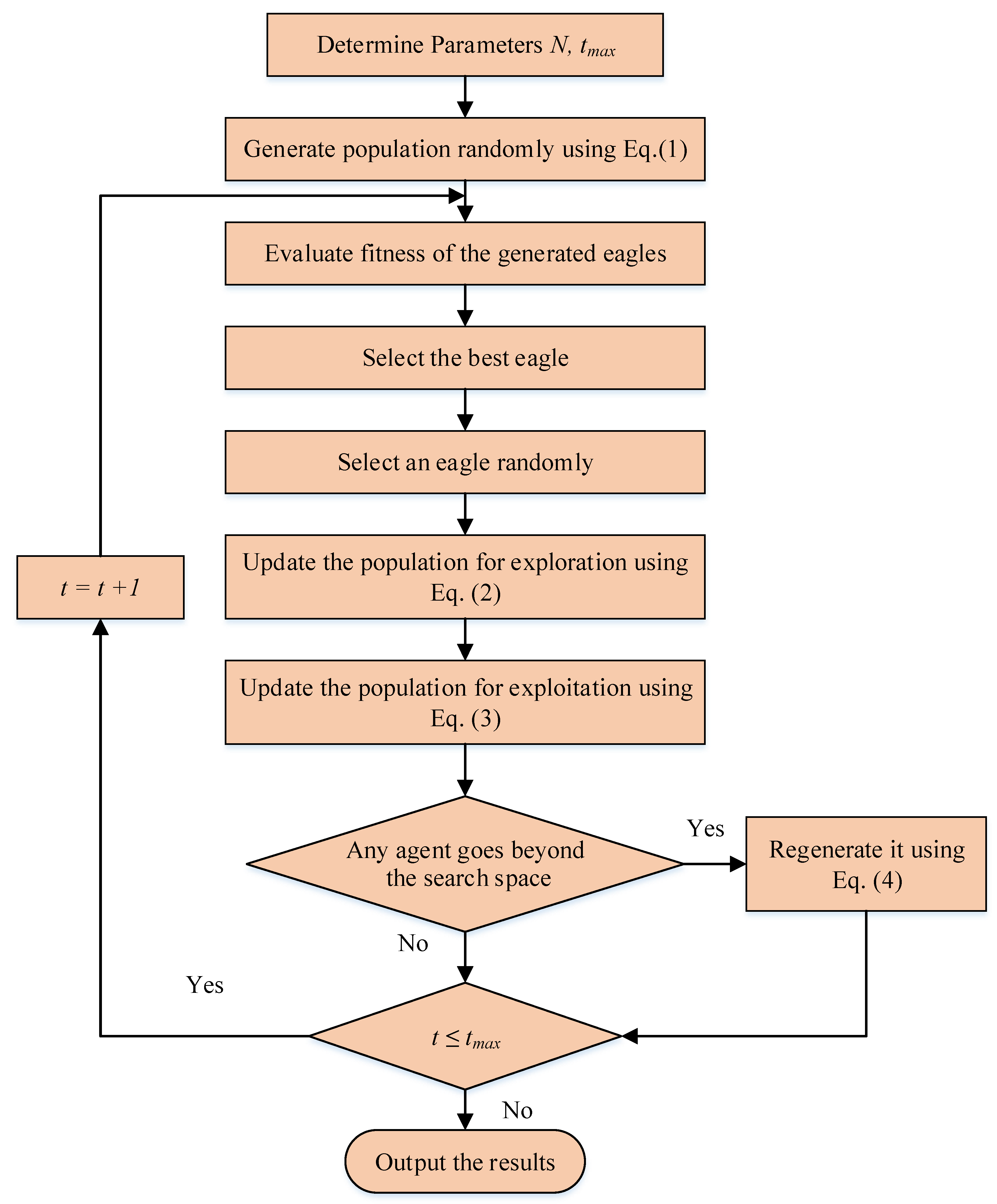
3. White-Tailed Eagle Algorithm (WEA)

The competitiveness of novel metaheuristics in solving optimization problems is a common criterion for their evaluation. It is important to note that it is not possible to develop an algorithm that can generate global solutions for all types of problems. The literature has indicated that metaheuristics are highly suitable for handling difficult problems. The "No Free Lunch" concept, however, encourages academics to develop innovative optimization algorithms to solve the real-life problems that inevitably arise owing to technological advancements [78]. This theory also holds this area of research open. Hence, there are still issues that have not yet been addressed or can be better addressed by new algorithms. Furthermore, there is no work in the literature that mimics the behavior of white-tailed eagles in nature.

The white-tailed eagle optimization algorithm is a population-based and gradient-free method, so it can be used to address complicated or straightforward optimization problems. The main advantages of the proposed WEA are its capacity to avoid local optima, explore the search region, and more reliably exploit the global optimum. Additionally, the method is relatively simple and easy to implement, with few parameters that need to be adjusted. In this section, the inspiration and mathematical model of the proposed WEA are presented, which is inspired by the social behavior and hunting mechanisms of white-tailed eagles in nature.

3.1. Inspiration and Behavior of White-Tailed Eagles

White-tailed eagles are sporadic predators who only exist at the top of the food chain due to their magnitude [79]. Moreover, these birds are scavengers who eat protein-rich foods. White-tailed eagles prefer to eat fish as their principal source of food, and they have the ability to detect fish from great distances [80]. White-tailed eagles use a variety of assault strategies and can hunt while flying. White-tailed eagles can change their foraging technique and move from passively waiting for prey to an active quest [81].

After that, white-tailed eagles take a break because hunting requires a lot of energy. These eagles fly in a predetermined direction and choose a specific region to begin their search for food above a body of water. As a result, self-searching and tracking other birds are used to locate the search space. Following that, white-tailed eagles will fly straight to the location. Because space searching is the first stage of hunting behavior, when the eagles arrive in the region, they will start looking for food [81]. Additionally, while soaring high, white-tailed eagles reap the benefits of stormy weather. Increased wind speed triggers soaring, during which eagles spend a significant amount of time flying. They have good vision as well, allowing them to see food under the water from hundreds of feet above. An eagle’s eye is the same size as a humans, but it has greater power. In addition, an eagle’s eye has excellent vision, four times higher than humans. Eagles may also realize in both forward and side views at the same time. Scanning gets simple with a twisting motion when eagles are flying thousands of feet in the air.

The next step of hunting behavior is going to the prey. When the eagles spot their meal, they begin the final step of their hunting activity, which involves descending with a slow flow of motion to approach the target at a high speed and snatching the fish from the water. To validate the sequences of each step of hunting, the proposed white-tailed eagle algorithm simulates the behavior of the white-tailed eagle during hunting. As a result, this algorithm can be broken down into two parts, namely, searching the search space and improving the population and moving toward the prey [79].

3.2. Optimization Algorithm

Even with the broad diversity of population-based methods, the process of reaching the optimum is almost the same. Typically, these algorithms begin the search with a randomly chosen initial population. Utilizing a fitness function, these randomly generated solutions are evaluated throughout iterations and improved using a set of formulae until a termination requirement is satisfied.

Regardless of differences between the population-based techniques, these methods share common information. In these approaches, the search process is divided into two stages: exploration and exploitation [82]. Exploration comprises searching the full search area for open locations that are far from the present position. The exploration stage occurs when a metaheuristic approach tries to identify the best areas of a given search space. On the other hand, the goal of exploitation is to explore the near-optimal points. During the exploitation stage, the algorithm might focus on the neighborhood of higher-quality answers inside the problem space. Implementation of the exploration alone could result in new positions with a poor degree of precision. Using exploitation solely, on the other hand, raises the risk of being stuck in local ideal situations. Numerous investigations have underlined the significance of balancing exploration and exploitation in metaheuristic approaches [83]. As a result, achieving the right balance among these two stages is vital. In the proposed WEA, two different phases are introduced to make an effective exploration and exploitation.

The proposed WEA’s step-by-step process is outlined below:

Step 1—Population initialization

As shown in the equation below, WEA, like other population-based evolutionary optimization approaches, starts the investigation by utilizing a collection of randomly generated elements (i.e., a set of eagles with a random position) in the search space.

$$E_i=l{b}_i+rand\times \left(u{b}_i-l{b}_i\right) ;i=1 ,2, \dots , N$$

(1)

The position of the ith eagle in the search space is represented by $E_i$. Furthermore, $u{b}_i$ and $l{b}_i$ represent the variable’s lower and upper limits, respectively. A random number between 0 and 1 is called rand.

Step 2—Population assessment

In the second stage, the created random solutions will be measured using the fitness function, and the eagle with the optimum fitness value will be chosen as $E_{Best}$.

Step 3—Searching phase (Exploration)

In this phase, white-tailed eagles look for prey within the searching area they’ve chosen, moving in different directions to speed up their hunt. Through the exploration of the search space, the algorithm carefully investigates various areas using its randomized operators. In this phase, each eagle cooperates with the best eagle and also interacts randomly with other eagles to update its position.

The following equation presents this behavior mathematically:

$$E_i\left(t+1\right)=\left\{\begin{array}{c}{E}_i\left(t\right)+2\times r_1\times \left(E_r\left(t\right)-E_i\left(t\right)\right) if r_2<0.5 \\ E_i\left(t\right)+2\times r_1\times \left(E_{Best}\left(t\right)-E_i\left(t\right)\right) if r_2\ge 0.5\end{array}\right.$$

(2)

where $E_i\left(t\right)$ represents the position of the ith eagle in the search space at iteration t, $E_r$ is position of the randomly selected eagle from the population (i ≠ r), $E_{Best}$ denotes the position of the best eagle (i.e., nearest eagle to the prey), r₁ and r₂ are random numbers in the range of (0, 1).

Step 4—Improving phase (Exploitation)

In the improving stage, each eagle gets knowledge from the population’s best candidate. In this phase, to improve the quality of the solutions of WEA, each eagle interacts with the best eagle of the swarm ($E_{Best}$). The best eagle has the greatest effect on others to find the prey. This behavior is illustrated in the following equation:

$$E_i\left(t+1\right)=rand\times E_{Best}\left(t\right)+rand\times \left(E_{Best}\left(t\right)-E_i\left(t\right)\right)$$

(3)

Step 5—Movement limitation

In every iteration, the WEA adjusts the distance each eagle moves through all dimensions of the scratch area. Equations (2) and (3) show that the eagles’ movement is a stochastic variable and can permit the eagle to follow a larger distance in the problem space. Therefore, to manage these oscillations and prevent the eagle’s divergence, any eagle that goes beyond the search-space limits will be regenerated according to the following equation:

$$E_i=\left\{\begin{array}{c}l{b}_i if E_i\le l{b}_i\\ u{b}_i if E_i\ge u{b}_i\\ E_i otherwise\\ \end{array}\right.$$

(4)

Algorithm 1 presents the proposed WEA’s pseudo code. In addition, the flowchart of the WEA is depicted in Figure 1.

Algorithm 1. White-Tailed Eagle Algorithm (WEA)

Determine the parameters N, tMax          Generate initial population of eagles using Equation (1)            Evaluate eagles’ fitness                 Rank the eagles based on their fitness                    Consider the best eagle as $E_{Best}$                t = 1                  while t < tMax                           Update the position of each eagle based on Equation (2)                           Move each eagle toward the prey using Equation (3)                           Check if any eagle goes beyond the                                       search space limit adjusts it                           Evaluate eagles’ fitness                           Rank the eagles based on their fitness                           Update $E_{Best}$                         t= t +1                  end while Output the best solution

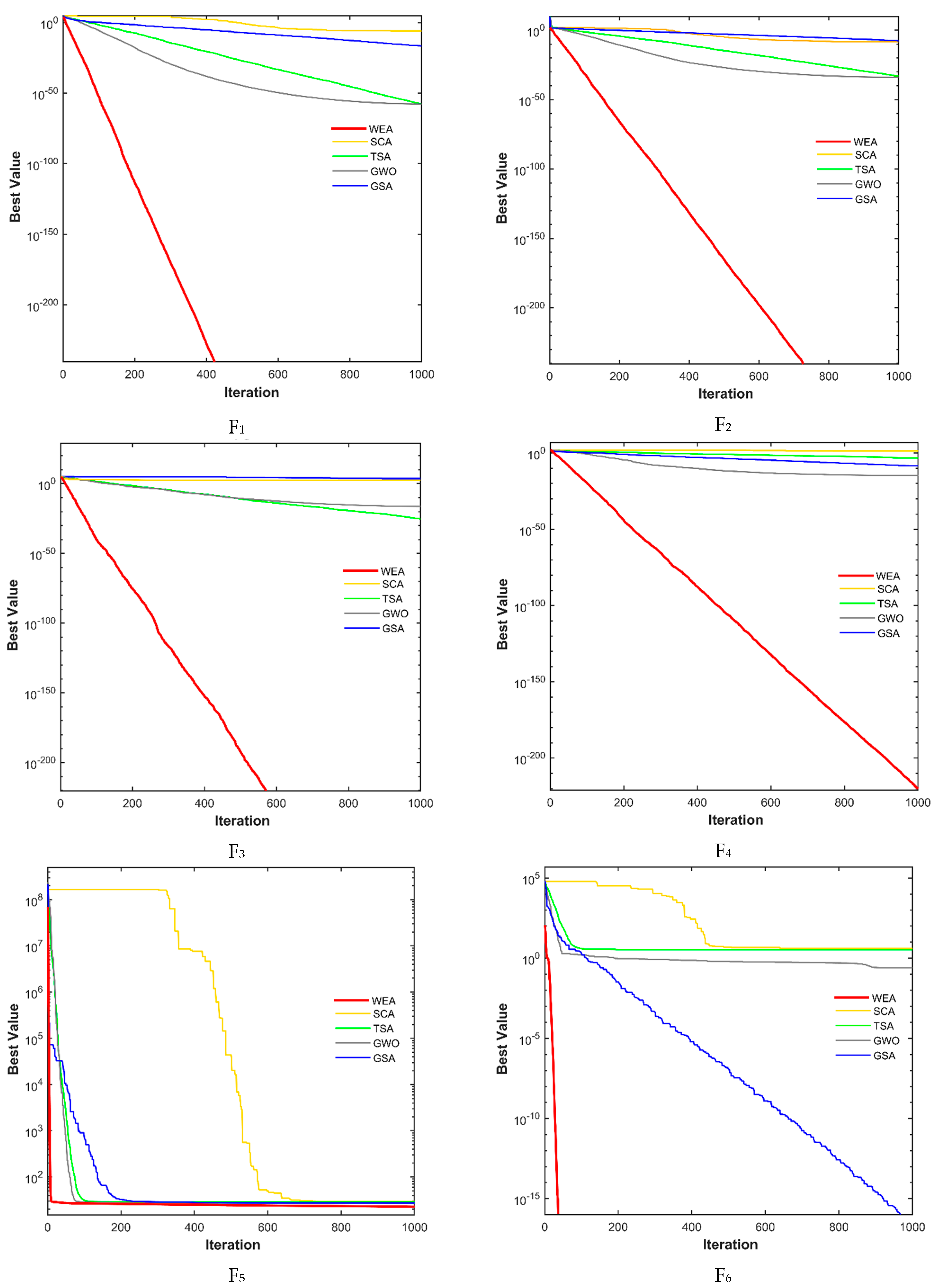
4. Comparative Analysis of the WEA

Because metaheuristic algorithms are stochastic, numerous test cases must be used to approve an algorithm’s efficacy. The performance of WEA is examined in this study using a well-studied set of benchmark problems from the literature [84,85], as well as a great combination of well-established algorithms. All of these are minimizing problems that may be used to assess the search efficiency and convergence rate of optimization algorithms.

Table 1. Unimodal benchmark functions.

Function	Range	${\mathit{f}}_{\mathit{m}\mathit{i}\mathit{n}}$	n (Dim)
$F_1\left(X\right)={{\displaystyle \sum }}_{i=1}^n{x}_i^2$	${\left[-100, 100\right]}^n$	0	30
$F_2\left(X\right)={{\displaystyle \sum }}_{i=1}^n\left|x_i\right|+{{\displaystyle \prod }}_{i=1}^n\left|x_i\right|$	${\left[-10, 10\right]}^n$	0	30
$F_3\left(X\right)={{\displaystyle \sum }}_{i=1}^n{\left({{\displaystyle \sum }}_{j=1}^i{x}_j\right)}^2$	${\left[-100, 100\right]}^n$	0	30
$F_4\left(X\right)=\underset{i}{\max } \left\{\left|x_i\right|, 1\le i\le n \right\}$	${\left[-100, 100\right]}^n$	0	30
$F_5\left(X\right)={{\displaystyle \sum }}_{i=1}^{n-1}\left[100{\left(x_{i+1}-x_i^2\right)}^2+{\left(x_i-1\right)}^2\right]$	${\left[-30, 30\right]}^n$	0	30
$F_6\left(X\right)={{\displaystyle \sum }}_{i=1}^n{\left(\left[x_i+0.5\right]\right)}^2$	${\left[-100, 100\right]}^n$	0	30
$F_7\left(X\right)={{\displaystyle \sum }}_{i=1}^{n}i{x}_i^4+random\left[0,1\right)$	${\left[-1.28, 1.28\right]}^n$	0	30

and

Table 2. Multimodal benchmark problems.

Function	Range	${\mathit{f}}_{\mathit{m}\mathit{i}\mathit{n}}$	n (Dim)
$F_8\left(X\right)={{\displaystyle \sum }}_{i=1}^n-x_i\sin \left(\sqrt{\left|x_i\right|}\right)$	${\left[-500, 500\right]}^n$	428.9829 × n	30
$F_9\left(X\right)={{\displaystyle \sum }}_{i=1}^n\left[x_i^2-10\cos \left(2\pi x_i\right)+10\right]$	${\left[-5.12, 5.12\right]}^n$	0	30
$$\begin{gathered} F_{10}\left(X\right)=-20 \exp \left(-0.2\sqrt{\frac{1}{n}{{\displaystyle \sum }}_{i=1}^n{x}_i^2}\right)- \\ \exp \left(\frac{1}{n}{{\displaystyle \sum }}_{i=1}^n\cos \left(2\pi x_i\right)\right)+20+e \end{gathered}$$	${\left[-32, 32\right]}^n$	0	30
$F_{11}\left(X\right)=\frac{1}{4000}{{\displaystyle \sum }}_{i=1}^n{x}_i^2-{{\displaystyle \prod }}_{i=1}^n\cos \left(\frac{x_i}{\sqrt{i}}\right)+1$	${\left[-600, 600\right]}^n$	0	30
$F_{12}\left(X\right)=$	${\left[-50, 50\right]}^n$	0	30
$$\begin{gathered} \frac{\pi }{n}\left\{10\sin \left(\pi y_1\right)+{{\displaystyle \sum }}_{i=1}^{n-1}{\left(y_i-1\right)}^2\left[1+10{\sin }^2\left(\pi y_{i+1}\right)\right]+{\left(y_n-1\right)}^2\right\} \\ \hspace{1em}\hspace{1em}\hspace{1em}\hspace{1em}\hspace{1em}\hspace{1em}\hspace{1em}\hspace{1em}+{{\displaystyle \sum }}_{i=1}^{n}u\left(x_i,10, 100, 4\right) \end{gathered}$$
$y_i=1+\frac{x_i+4}{4}$$, u\left(x_i,a, k, m\right)=\left\{\begin{array}{c}k{\left(x_i-a\right)}^m x_i>a \\ 0 a<x_i<a \\ k{\left(-x_i-a\right)}^m x_i<-a\end{array}\right.$
$$\begin{gathered} F_{13}\left(X\right)=0.1\left\{{\sin }^2\left(3\pi x_1\right) \\ \hspace{1em}\hspace{1em}\hspace{1em}\hspace{1em}\hspace{1em}\hspace{1em}\hspace{1em} +{{\displaystyle \sum }}_{i=1}^n{\left(x_i-1\right)}^2\left[1+{\sin }^2\left(3\pi x_i+1\right)\right] \\ \hspace{1em}\hspace{1em}\hspace{1em}\hspace{1em}\hspace{1em}\hspace{1em}\hspace{1em} +{\left(x_n-1\right)}^2\left[1+{\sin }^2\left(2\pi x_n\right)\right]\right\}+{{\displaystyle \sum }}_{i=1}^{n}u\left(x_i,5, 100, 4\right) \end{gathered}$$	${\left[-50, 50\right]}^n$	0	30

provide the details and mathematical formulation of these test functions [63]. Figure 2 and Figure 3 show three-dimensional illustrations of these benchmark functions.

This benchmark set is divided into two categories: unimodal test functions with a single global best for evaluating an algorithm’s convergence rate and exploitation capability, and multimodal test functions by numerous local solutions and a global optimum for evaluating an algorithm’s local optima prevention and exploration power. The suggested algorithm is written in the computer language MATLAB R2020b. After the manuscript is accepted, the MATLAB code will be published. It is advised that the performance of a newly presented computational intelligence algorithm be compared to the performance of other generally established algorithms in the area in order to validate its success.

The suggested WEA’s findings and performance are compared to those of other well-known optimization techniques. The WEA has a simple structure and requires just two key parameters: the number of eagles (N) and the maximum iteration number (t_Max). Actually, the termination criterion of the algorithm is the maximum number of iterations.

The primary parameters of the algorithms under consideration are shown in

Table 3. Selected algorithms’ parameters.

Algorithm (Year)	Parameter	Value
WEA (2022)	Number of eagles	50
	Iterations’ Number	1000
GSA (2009)	Agent’s Number	50
	Gravitational constant	100
	Iterations’ Number	1000
GWO (2014)	Agent’s Number	50
	Control parameter	[2,0]
	Iterations’ Number	1000
SCA (2016)	Agent’s Number	50
	Number of elites	2
	Iterations’ Number	1000
TSA (2020)	Agent’s Number	50
	Iterations’ Number	1000

. These coefficients were obtained using the reference-based parameter detection approach, as advised by the authors of the original studies.

Because metaheuristic strategies are stochastic, the outcomes of a single run may not be accurate, and the methods can seek better or even worse answers than those previously found. Thus, to obtain a proper assessment and efficacy measurement of the techniques, statistical analysis is used. To deal with this problem, thirty separate runs are done for the specified approaches, and statistical findings are obtained and given in

Table 4. Results of unimodal test problems.

Fun.	Index	WEA	TSA	SCA	GSA	GWO
F1	Min	0.00	5.238 × 10−61	1.613 × 10−7	1.128 × 10−17	2.513 × 10−61
	Max	0.00	1.218 × 10−54	2.931 × 10−3	3.243 × 10−17	3.754 × 10−58
	Avg	0.00	8.245 × 10−56	2.298 × 10−4	2.276 × 10−17	4.817 × 10−59
	Med	0.00	7.221 × 10−58	1.887 × 10−5	2.105 × 10−17	1.132 × 10−59
	SD	0.00	2.520 × 10−55	7.875 × 10−4	5.921 × 10−18	1.144 × 10−58
F2	Min	0.00	1.029 × 10−35	1.485 × 10−9	1.473 × 10−8	8.412 × 10−36
	Max	0.00	3.321× 10−32	9.796 × 10−6	3.419 × 10−8	5.295 × 10−34
	Avg	0.00	2.233 × 10−33	1.732 × 10−6	2.465 × 10−8	8.421 × 10−35
	Med	0.00	3.224 × 10−34	5.342 × 10−7	2.497 × 10−8	5.891 × 10−35
	SD	0.00	6.133 × 10−33	2.316 × 10−6	3.898 × 10−9	9.789 × 10−35
F3	Min	0.00	2.575 × 10−32	70.8285	102.955	1.311 × 10−19
	Max	0.00	2.452 × 10−17	267.0	468.616	3.499 × 10−13
	Avg	0.00	8.182 × 10−19	789.1620	245.469	1.488 × 10−14
	Med	0.00	1.871 × 10−24	619.4506	221.115	2.132 × 10−17
	SD	0.00	4.468 × 10−18	746.2287	100.102	6.612 × 10−14
F4	Min	6.02 × 10−224	3.318 × 10−8	1.2610	2.312 × 10−9	9.716 × 10−16
	Max	3.82 × 10−218	6.419 × 10−5	35.6743	5.123 × 10−9	2.332 × 10−13
	Avg	6.27 × 10−219	1.222 × 10−5	9.3080	3.221 × 10−9	1.872 × 10−14
	Med	7.98 × 10−220	2.110 × 10−6	6.9806	3.191 × 10−9	6.412 × 10−15
	SD	0.00	1.717 × 10−5	8.0720	7.398 × 10−10	4.886 × 10−14
F5	Min	22.441	25.6273	27.3230	25.745	25.2273
	Max	22.945	29.5430	49.5110	220.911	28.7294
	Avg	22.646	28.4422	29.9106	42.2647	26.9256
	Med	22.624	28.8115	29.0097	26.1443	27.1173
	SD	0.163	0.7616	4.1508	45.4674	0.8418
F6	Min	0.00	2.0585	3.4070	9.669 × 10−18	0.2466
	Max	0.00	4.7791	4.4435	8.712 × 10−16	1.2619
	Avg	0.00	3.6724	4.0360	3.123 × 10−17	0.6376
	Med	0.00	3.5615	4.0572	2.889 × 10−17	0.7452
	SD	0.00	0.6918	0.2954	6.214 × 10−18	0.3353
F7	Min	9.764 × 10−6	6.711 × 10−4	0.0015	0.0061	1.492 × 10−4
	Max	1.459 × 10−4	0.0036	0.0431	0.0462	2.132 × 10−3
	Avg	5.385 × 10−5	0.0018	0.0116	0.0237	7.885 × 10−4
	Med	5.271 × 10−5	0.0018	0.0078	0.0222	7.111 × 10−4
	SD	3.772 × 10−5	7.726 × 10−4	0.0101	0.0098	4.711 × 10−4

and

Table 5. Results of multimodal test problems.

Fun.	Index	WEA	TSA	SCA	GSA	GWO
F8	Min	−1.242 × 104	−7.776 × 103	−5.341 × 103	−3.713 × 103	−8.964 × 103
	Max	−1.182 × 104	−5.324 × 103	−3.449 × 103	−2.122 × 103	−4.888 × 103
	Avg	−1.204 × 104	−6.598 × 103	−4.143 × 103	−2.654 × 103	−6.161 × 103
	Med	−1.193 × 104	−6.599 × 103	−3.886 × 103	−2.854 × 103	−6.155 × 103
	SD	88.432	600.1324	341.645	359.543	848.243
F9	Min	0.00	77.7761	1.0560 × 10−6	8.9546	0.00
	Max	0.00	254.9883	51.4451	21.8891	10.0548
	Avg	0.00	151.4539	5.9694	15.6209	0.8853
	Med	0.00	149.6596	9.3391 × 10−4	15.9193	0.00
	SD	0.00	35.8717	12.2476	3.1043	2.4438
F10	Min	8.882 × 10−16	1.5099 × 10−14	1.5579 × 10−5	2.612 × 10−9	1.321 × 10−14
	Max	4.441 × 10−15	4.3125	20.2198	4.325 × 10−9	2.314 × 10−14
	Avg	2.664 × 10−15	2.4095	14.3622	3.513 × 10−9	1.623 × 10−14
	Med	2.664 × 10−15	2.9381	20.1275	3.524 × 10−9	1.445 × 10−14
	SD	1.872 × 10−15	1.3920	8.9778	5.211 × 10−10	2.643 × 10−15
F11	Min	0.00	0.00	4.8381 × 10−7	1.6952	0.00
	Max	0.00	0.0159	0.7703	10.6642	0.0140
	Avg	0.00	0.0077	0.1368	4.2510	0.0014
	Med	0.00	0.0082	0.0032	3.5667	0.00
	SD	0.00	0.0057	0.2218	2.0234	0.0041
F12	Min	1.571 × 10−32	0.2738	0.2631	8.203 × 10−2	0.0121
	Max	1.909 × 10−32	13.8088	5.6300	0.1037	0.0920
	Avg	1.626 × 10−32	6.3735	0.9568	0.0198	0.0364
	Med	1.578 × 10−32	6.7411	0.4964	1.3512	0.0329
	SD	1.086 × 10−33	3.4586	1.1497	0.0400	0.0201
F13	Min	1.342 × 10−32	1.7796	1.8452	1.291 × 10−18	0.1006
	Max	2.046 × 10−31	4.1077	22.5849	0.022	1.0416
	Avg	6.44 × 10−32	2.8976	3.4211	7.198 × 10−4	0.5280
	Med	3.075 × 10−32	2.8914	2.3552	2.034 × 10−18	0.5238
	SD	7.528 × 10−32	0.6436	3.9911	3.011 × 10−3	0.2359

. The exploitation, exploration, and convergence rate of the novel approach are studied, utilizing a comparison of WEA versus four chosen algorithms, in the following subsections.

4.1. Exploitation Validation

Unimodal test problems can be used to assess an optimization algorithm’s exploitation capabilities [86,87]. In order to assess the WEA’s ability to exploit encouraging regions, seven unimodal benchmark problems presented in Table 1 are considered. The findings are compared to other approaches in Table 4. The findings presented in this table suggest that the WEA might offer a better solution for all unimodal tasks. The WEA also reached the global optima for four functions (F₁, F₂, F₃, F₆). In comparison to other optimization methods, the obtained results suggest that the novel approach has a vast potential search capacity.

4.2. Exploration Verification

Multiple local optima in multimodal benchmark functions examined the capacity of an optimization approach to properly explore the search area [86,87]. There is a minimization of six multimodal functions (F₈ to F₁₃) in this study using the presented method. Table 5 show that the Best and Mean values obtained by the WEA for all problems are much better than those obtained by the other methods. Additionally, when compared to the other strategies, the findings indicate that the WEA is a more reliable method in terms of standard deviation.

Based on the results of the investigation, the WEA either outperforms or performs almost equally with the other algorithms. The consistent performance of the new technique across such a wide range of multi-modal benchmark functions confirms its superior exploration capabilities.

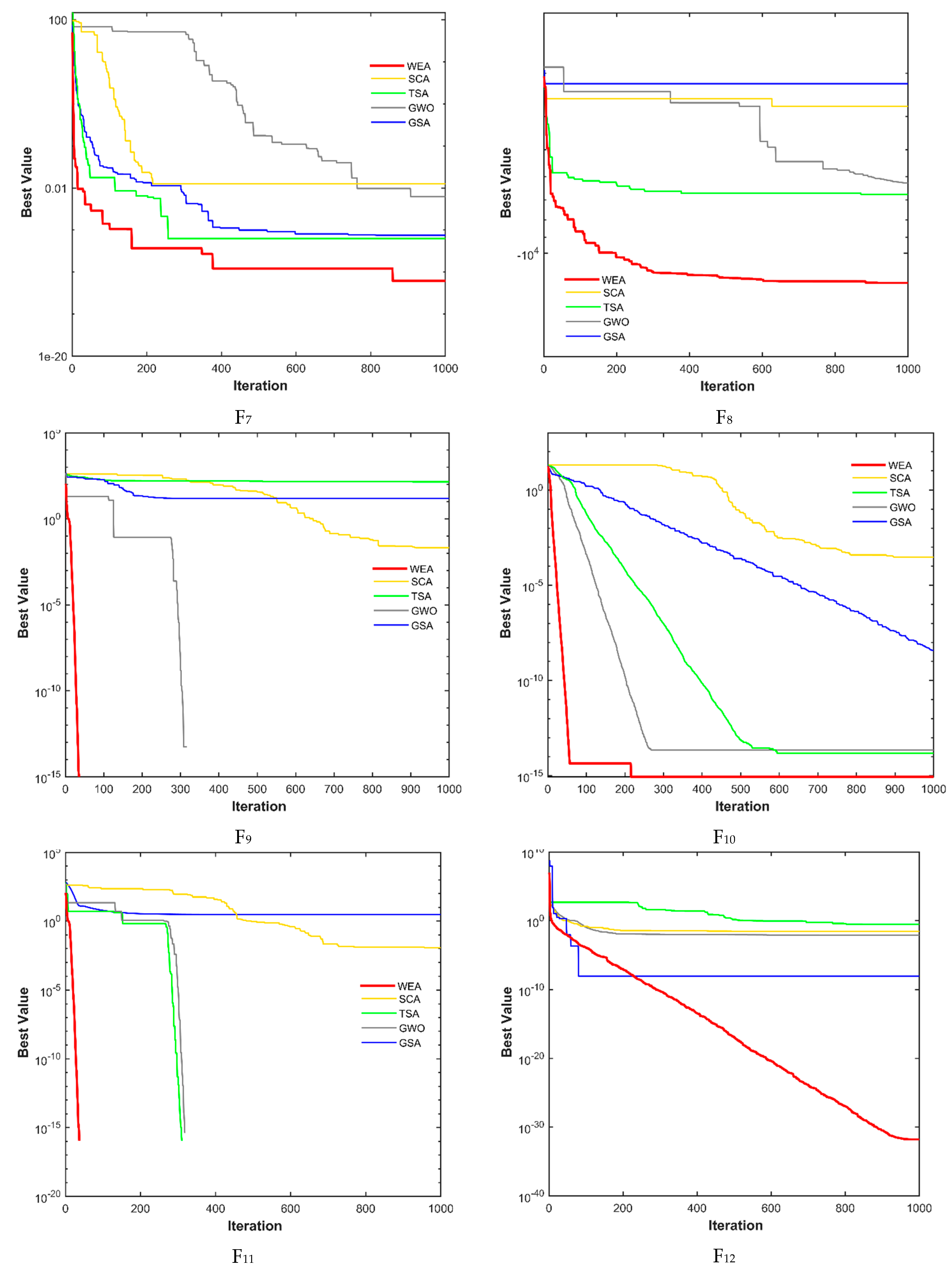
4.3. Convergence Ability

A successful optimization technique needs to reach the global best solution rather than settling for a local optimum in early iterations. In Figure 4, the convergence progress curves of the WEA are compared to GSA, SCA, TSA, and GWO for certain benchmark test functions. The curves are displayed versus the number of iterations, which ranges from hundreds to thousands.

In most problems, the WEA outperforms the other algorithms, as seen in the graph. The test function optimization curves reveal that the WEA is proficient in exploring the search space and discovering the problem’s area in fewer iterations.

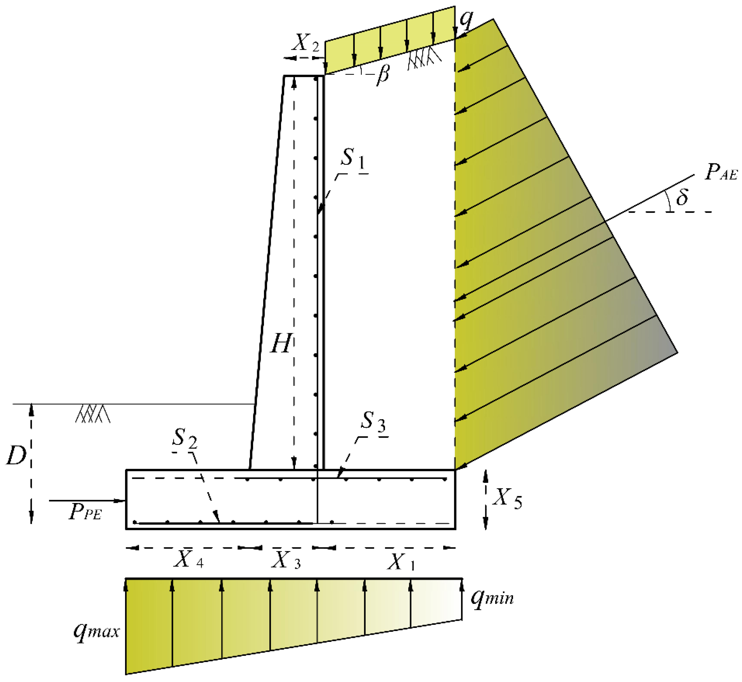
5. Retaining Structure Analysis

One of the essential issues in civil engineering is the seismic evaluation of the retaining structures. Reinforced concrete retaining walls are one of the most widely used structures in various projects such as supporting excavations, road construction, and bridge abutments. However, when seismic loads are applied, it will be more difficult to assess the precise behavior of these structures. Therefore, to evaluate how the structure will respond to seismic loads, an efficient pseudo-static approach will be used.

The Mononobe-Okabeh (M-O) is a common pseudo-static technique for determining the distribution of earthquake pressure [88]. A one-meter-long retaining structure subject to general forces is shown in Figure 5. The active and passive earth pressures under earthquake loads are shown in this figure as P_AE and P_PE, respectively. H stands for the wall’s overall height, β for the angle of backfill slope, D for the soil depth, q for the surcharge load, and q_min and q_max for the contact pressure’s minimum and maximum values.

The analysis of retaining structures begins with a determination of the active and passive earth pressure applied on a wall. The M-O theory states that the following equations can be used to determine a total active earth force [88]:

$$P_{AE}=\frac{1}{2}\gamma H^2\left(1-K_V\right)K_{AE}$$

(5)

$$K_{AE}=\frac{si{n}^2\left(\varnothing +\alpha -\theta \right)}{\cos \left(\theta \right)si{n}^2\left(\alpha \right)sin\left(\alpha -\delta -\theta \right){\left[1+\sqrt{\frac{\sin \left(\delta +\varnothing \right)\sin \left(\varnothing -\theta -\beta \right)}{\sin \left(\alpha -\delta -\theta \right)\sin \left(\alpha +\beta \right)}}\right]}^2}$$

(6)

where, 𝛼 denotes the angle of the wall’s back face and θ denotes the angle of seismic inertia that can be obtained by:

$$\theta ={\tan }^{-1}\left(\frac{K_h}{1-K_V}\right)$$

(7)

According to the definitions below, K_V and K_h represent the vertical and horizontal acceleration constants:

$$K_h=\frac{horizontal earthquake acceleration component}{acceleration due to gravity \left(g\right)}$$

(8)

$$K_V=\frac{vertical earthquake acceleration component}{acceleration due to gravity \left(g\right)}$$

(9)

The M-O theory states that the following formula can be applied to calculate the total passive earth force under earthquake loads [88]:

$$P_{PE}=\frac{1}{2}\gamma H^2\left(1-K_V\right)K_{PE}$$

(10)

$$K_{PE}=\frac{{\sin }^2\left(\alpha -\varnothing -\theta \right)}{\cos \left(\theta \right){\sin }^2\left(\alpha \right)\sin \left(\alpha +\delta -\theta \right){\left[1-\sqrt{\frac{\sin \left(\delta +\varnothing \right)\sin \left(\varnothing +\beta -\theta \right)}{\sin \left(\alpha +\delta -\theta \right)\sin \left(\alpha +\beta \right)}}\right]}^2}$$

(11)

6. Optimization of Retaining Structure

In the optimal design problem, the objective function f is to be minimized while taking into account the constraints g, which are represented by Equation (12)

$$minimize f\left(X\right) X=\left[x_1,x_2, \dots , x_n\right]$$

(12)

$$subject to g_i\left(X\right)\le 0 i=1, 2, \dots . m{X}^L\le X\le X^U$$

where, X is a vector containing the n design variables; g(X) is a vector containing the m inequality constraints. The design variables’ lower and upper bounds are represented by the two vectors, X^L and X^U, respectively. The design variables, the objective function, and the design constraints related to the optimization of retaining structures are presented in the following.

6.1. Objective Function

In the present research, the embedded CO₂ emission and construction price of the structure that is subject to both static and dynamic loads are taken into consideration as objective functions. Therefore, the goal is to reduce the value of one of these two objective functions. The volume of concrete, excavation, compacted backfill, formwork, and reinforcing steel are considered by both objective functions. The following equation shows the structure’s overall cost:

$$f_{cost}=C_s{W}_{st}+C_c{V}_c+C_e{V}_e+C_f{A}_f+C_b{V}_b$$

(13)

where, V_c, V_e, and V_b represent the volumes of concrete, excavation, and backfill, and W_st is the steel bars weight. A_f displays the formwork area. The unit prices of excavation (C_e), formwork (C_f), reinforcement (C_s), backfill (C_b), and concrete (C_c), are presented in

Table 6. Retaining walls assembly unit price.

Item	Notaition	Unit	CO2 Emission	Unit Cost
Excavation	Ve	m3	13.16 Kg	11.41 $
Formwork	Af	m2	31.66 Kg	37.08 $
Reinforcement	Wst	kg	2.82 Kg	1.51 $
Backfill	Vb	m3	27.20 Kg	38.10 $
Concrete	Vc	m3	224.34 Kg	99.49 $

[12].

The following equation is a form of the next objective, which quantifies the total CO₂ emissions of retaining walls:

$$f_{co2}=E_s{W}_{st}+E_c{V}_c+E_e{V}_e+E_f{A}_f+E_b{V}_b$$

(14)

Table 6 presents the unit CO₂ emissions of excavation (E_e), formwork (E_f), reinforcement (E_s), backfill (E_b), and concrete (E_c) [12].

6.2. Design Variables

The eight continuous design variables taken into account in this study include three variables that represent the steel reinforcement of various structural components and five others that relate to the geometry of the structure shown in Figure 5. In this figure, X₁ represents the heel’s width, X₂ stand for the top stem thickness, X₃ for the bottom stem thickness, X₄ for the toe’s width, and X₅ represents the base slab’s thickness. S₁ represents the stem’s vertical reinforcement, S₂ represents the toe’s horizontal reinforcement, and S₃ represents the heel’s horizontal reinforcement.

6.3. Design Constraints

The restrictions on stability and strength imposed by the American Concrete Institute’s design code (ACI 318−05) [89], taken into account in the retaining structures optimization are presented below:

• Overturning Stability Constraint:

  $$\frac{\mathrm{total} \mathrm{resistant} \mathrm{moments}}{\mathrm{total} \mathrm{overturning} \mathrm{moments}}\ge F{S}_{Odesign}{}_{}$$

  (15)

  where, FS_Odesign is prescribed factors of safety against overturning.
• Sliding stability constraint:

  $$\frac{total horizontal resistant forces}{total horizontal driving forces}\ge F{S}_{Sdesign}{}_{}$$

  (16)

  where, FS_Sdesign is prescribed factors of safety against sliding.
• Bearing capacity constraint:

  $$\frac{q_u}{q_{max}}\ge F{S}_{Bdesign}$$

  (17)

  where, q_u is the ultimate bearing capacity obtained by the Meyerhof Bearing Capacity Theory [90]; q_max is the maximum applied bearing stress. The maximum and minimum contact pressure are defined in the following equation:

  $$q_{max,min}=\frac{\sum V}{B}\left(1\pm \frac{6e}{B}\right)$$

  (18)

  where, ∑V denotes the total vertical forces, B denotes the width of foundation, and e denotes the load’s eccentricity.
• No tension at the foundation:

  $$q_{min}\ge 0$$

  (19)
• Moment capacity of toe, heel and bottom of stem:

  $$M_u\le 0.9A_s{f}_y\left(d-0.5\times \frac{A_s{f}_y}{0.85f_{c}b}\right)$$

  (20)

  where, M_u is the ultimate bending moment, f_c is the compressive concrete strength, and f_y is the steel yield strength.
• Shear capacity of toe, heel, and stem:

  $$V_u\le \frac{1}{6}0.75\sqrt{f_c}bd$$

  (21)

  where, V_u is ultimate shearing force
• Limitation of flexural reinforcement:

  $${\rho }_{min}\le \rho \le {\rho }_{max} , \rho =\frac{A_s}{bd}, {\rho }_{min}=\frac{1.4}{fy} , {\rho }_{max}=\left(\frac{{0.85}^2{f}_c}{f_y}\right)\left(\frac{600}{600+f_y}\right)$$

  (22)

In this research, a penalty function approach is employed to take into account the above restrictions and convert a constrained optimization to an unconstrained problem based on the following equation:

$$F\left(X\right)=f\left(X\right)+r{{\displaystyle \sum }}_{i=1}^{p}max{\left\{0,g_i\left(X\right)\right\}}^l$$

(23)

where, F(X) represents the penalized objective function, f(X) denotes the the pictures.problem’s original objective function as stated in Equation (13) and Equation (14), and g(X) represents the problem’s constraints. The penalty factor, r, is considered equal to 1000, and the power of the penalty function, l, is considered equal to 2.

7. Model Validation

In this section, to validate the performance of the proposed method, a numerical example of a retaining structure is considered from the literature [58].

Table 7. Input parameters for numerical investigation.

Parameter	Unit	Symbol	Value
Height of stem	m	H	3.0
Internal friction angle of retained soil	degree	φ	36
Internal friction angle of base soil	degree	φ’	0.0
Unit weight of retained soil	kN/m3	γs	17.5
Unit weight of base soil	kN/m3	γ’s	18.5
Unit weight of concrete	kN/m3	γc	23.5
Unit weight of steel	kN/m3	γsteel	78.5
Cohesion of base soil	kPa	c	125
Depth of soil in front of wall	m	D	0.5
Surcharge load	kPa	q	20
Backfill slop	degree	𝛽	10
Concrete cover	cm	dc	7.0
Yield strength of reinforcing steel	MPa	fy	400
Compressive strength of concrete	MPa	fc	21
Shrinkage and temporary reinforcement percent	-	ρst	0.002
Design load factor	-	LF	1.7
Factor of safety for overturning stability	-	FSO	1.5
Factor of safety against sliding	-	FSS	1.5
Factor of safety for bearing capacity	-	FSB	3.0

lists the input parameters.

The big bang-big crunch optimization (BB-BC) was used by Camp and Akin [58] to solve this problem. Moreover, the interior search algorithm (ISA) was developed by Gandomi et al. [91] to find the answer. However, these studies found the solution subjected to the static loads. In the aforementioned studies, the following objective function is considered, which is based on the cost of steel and concrete:

$$f_{cost}=C_s{W}_{st}+C_c{V}_c$$

(24)

To justify the accuracy of the presented technique for optimization of retaining walls, the problem is solved based on the objective function presented in Equation (24) using the proposed WEA and the results are compared with BB-BC and ISA in

Table 8. Comparison of the optimum results of different algorithms.

Design Variable	Unit	Optimum Values WEA (Current Study)	Optimum Values BB-BC [58]	Optimum Values ISA [91]
heel’s width (X1)	m	0.65	0.8732	0.8023
top stem thickness (X2)	m	0.2	0.2	0.2
bottom stem thickness (X3)	m	0.272	0.2678	0.2875
toe’s width (X4)	m	0.68	0.6017	0.7536
base slab’s thickness (X5)	m	0.2722	0.2722	0.27
stem’s vertical reinforcement (S1)	cm2/m	12	12	13
toe’s horizontal reinforcement (S2)	cm2/m	8	8	7
heel’s horizontal reinforcement (S3)	cm2/m	8	8	7
Best Cost	$/m	68.76	70.96	73.05

.

As per the findings reported in Table 8, the optimal solution found by WEA is 68.76 $/m, which is slightly less costly than the design evaluated by BB-BC [58] and 5% cheaper than the ISA method. The results verify the new algorithm’s efficacy for optimization of retaining structures.

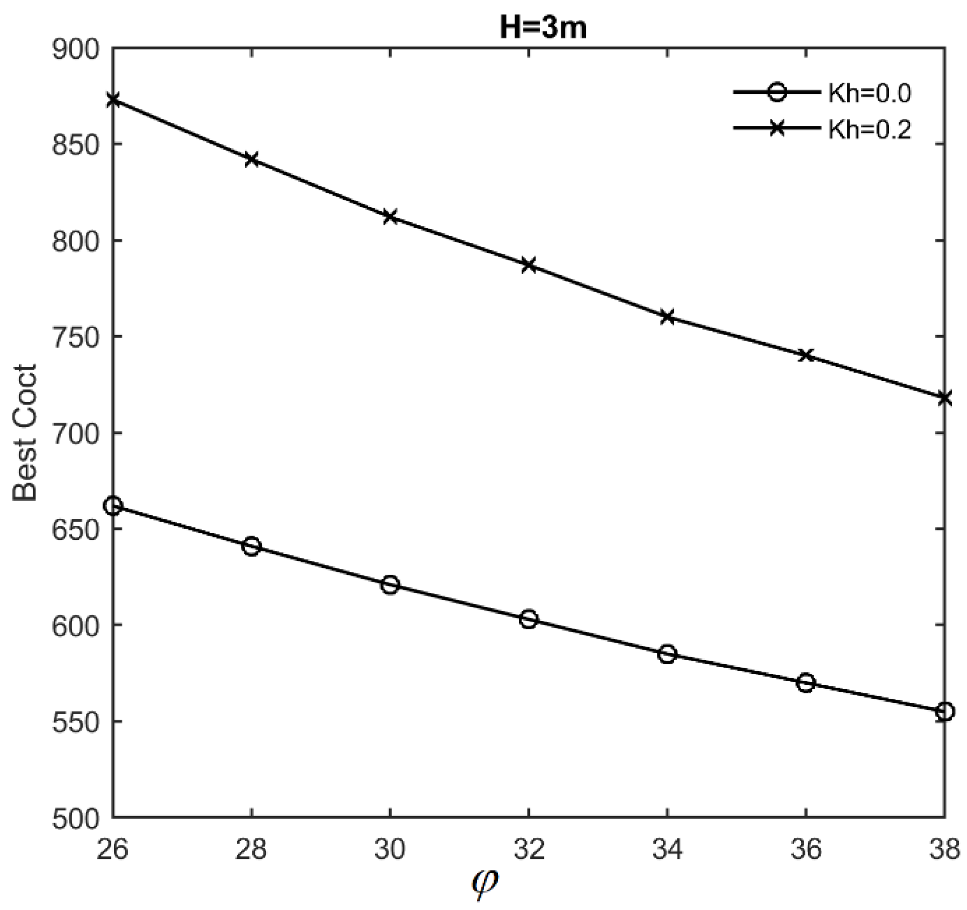
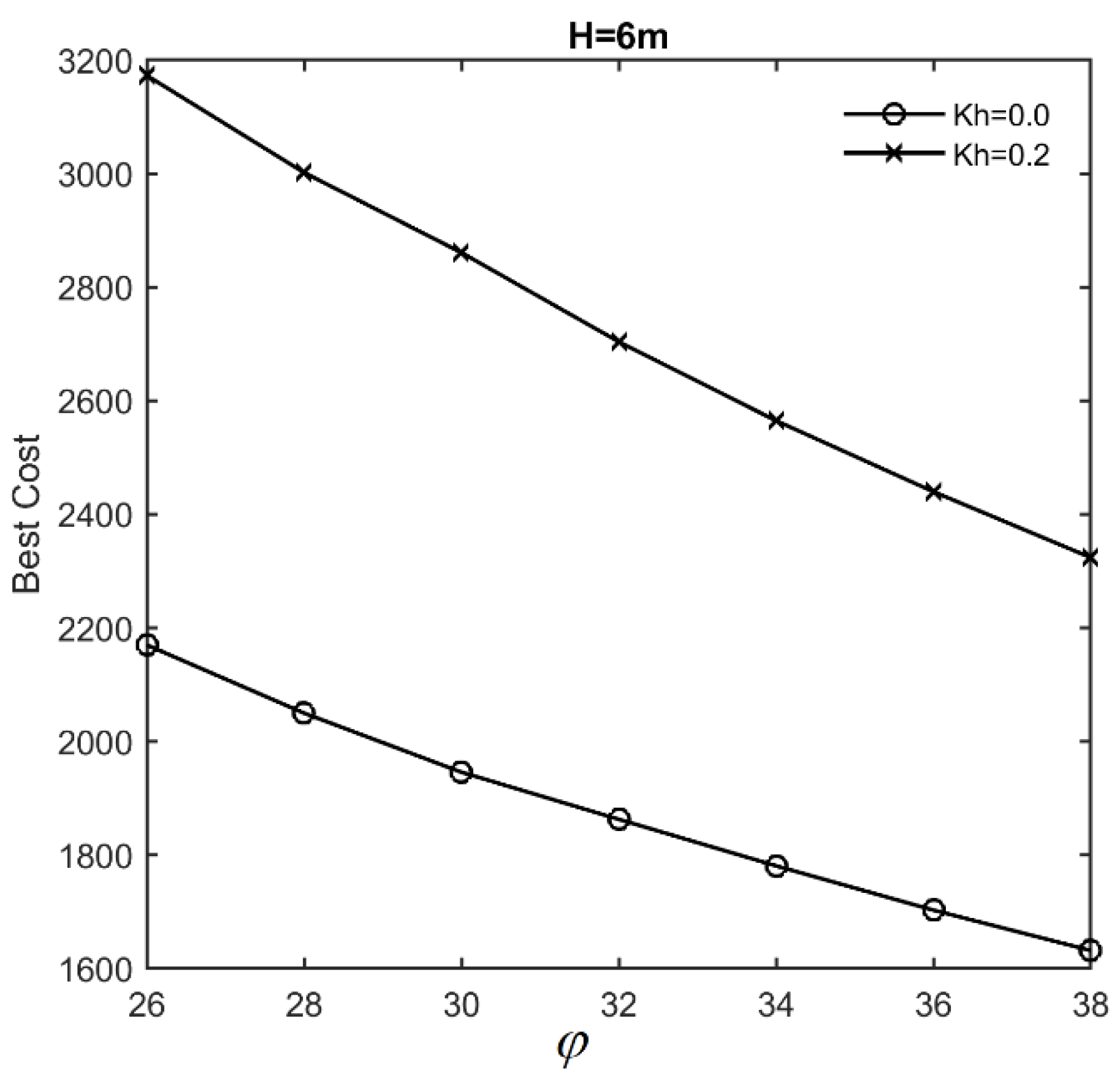
8. Model Application and Parametric Study

In this section, a numerical example of retaining structure optimization is considered from the study of Camp and Akin [58]. The input parameters are presented in Table 7. This experiment considers two objective functions as presented in Equation (13) and Equation (14): CO₂ emission and construction cost. The results of the cost and emission optimization are compared with each other. To investigate the effect of the horizontal and vertical acceleration coefficients on the total cost and CO₂ emission of the wall, a set of six different combinations of K_h and K_V have been considered as presented in

Table 9. Horizontal and vertical acceleration coefficient combinations.

Case No.	Case 1	Case 2	Case 3	Case 4	Case 5	Case 6
Kh	0.0	0.1	0.1	0.2	0.2	0.2
KV	0.0	0.0	0.1	0.0	0.1	0.2

.

The problem is solved using the WEA algorithm for different combinations of horizontal and vertical acceleration coefficients as presented in Table 9. The algorithm is run thirty times, and the optimum results for low-cost and low-CO₂ objectives are presented in

Table 10. Optimization result for cost objective function.

Design Variable	Unit	Optimum Values Case 1	Optimum Values Case 2	Optimum Values Case 3	Optimum Values Case 4	Optimum Values Case 5	Optimum Values Case 6
X1	m	0.5513	0.6539	0.613	0.7923	0.7887	0.7672
X2	m	0.2	0.2	0.2	0.2	0.2	0.2
X3	m	0.3567	0.0.3743	0.3686	0.3617	0.3364	0.3387
X4	m	0.7778	0.7632	0.7778	0.7778	0.7778	0.7778
X5	m	0.2727	0.2847	0.2821	0.2995	0.2997	0.2921
S1	cm2/m	8	8	8	9	9	8
S2	cm2/m	8	9	8	11	10	10
S3	cm2/m	8	9	10	11	10	10
Best Cost	$/m	572.74	599.3	593.1	641.3	631.91	622.73

and

Table 11. Optimization result for CO₂ objective function.

Design Variable	Unit	Optimum Values Case 1	Optimum Values Case 2	Optimum Values Case 3	Optimum Values Case 4	Optimum Values Case 5	Optimum Values Case 6
X1	m	0.6074	0.7113	0.6835	0.862	0.7993	0.7825
X2	m	0.2	0.2	0.2	0.2	0.2	0.2
X3	m	0.2929	0.304	0.3064	0.2841	0.3251	0.32
X4	m	0.7631	0.7635	0.75	0.7735	0.7777	0.7778
X5	m	0.2728	0.2775	0.2734	0.2907	0.2928	0.2901
S1	cm2/m	10	10	10	11	9	9
S2	cm2/m	8	9	9	11	10	10
S3	cm2/m	8	9	9	11	10	10
Best CO2	kg/m	740.1	773.33	762.09	822.35	812.35	805.11

, respectively.

The results of Table 10 indicate that the best price for the first case (no seismic loading) is 572.74 $/m. By increasing the K_h to 0.1 (case 2), the price will rise by 4.7%. When K_V is equal to 0.1 (case 3), the best cost slightly decreases, as it was predicted from Equation (1). In addition, by increasing K_h from 0 to 0.2 (case 4), the best cost increases by 12%, approximately. In cases 5 and 6, by increasing the value of K_V to 0.2, the construction cost will be decreased by up to 1.5%. According to these results, ignoring the K_V is acceptable under the general seismic optimization conditions for the retaining structure.

Similarly, in the case of CO₂ optimization, the results of Table 11 reveal that the total amount of CO₂ emissions will be increased by up to 4.5% and 11.1%, whereas the horizontal acceleration coefficient varies from zero to 0.1 and 0.2, respectively.

A sensitivity analysis was performed on a set of different wall heights from 3 to 11 m with increments of 1 m to assess the impact of the horizontal acceleration coefficient on the cost and CO₂ emission when the vertical acceleration coefficient is equal to zero. Figure 6 and Figure 7 show the parabolic curves of cost and CO₂ emission versus different wall heights, respectively.

As shown in Figure 6, the construction cost increases drastically as the height of the wall increases. However, the intensity of variation will be increased while K_h is equal to 0.2. The construction cost adjusts to Cost = 64.25H² − 234.8H + 755.2 with R² = 0.9994 for K_h = 0.0 and it is equal to Cost = 130.2H² − 770H + 1951 with R² = 0.9953 for K_h = 0.2. The results of CO₂ emissions presented in Figure 7 are also comparable with the results of the cost objective function. As shown in this figure, by increasing the height of the wall to 11m, the differences between the amount of CO₂ emission increases by up to 60%.

Figure 8 and Figure 9 show the low-CO₂ emission and low-cost designs of a wall with a height of 3 m for various values of K_h as the friction angle of the retained soil varies from 28 to 36 degrees. Over this range, for K_h equal to 0.0 and 0.2, both the low-cost and low- CO₂ emission designs decrease by approximately 19% as the friction angle increases.

Figure 10 and Figure 11 depict the low-CO₂ emission and low-cost designs of a 6 m-height wall for various values of the friction angle of the retained soil. As shown in these figures, the low-cost designs decrease by 26% as the friction angle increases, whereas the low-CO₂ emission designs decrease by 30%. These findings indicate that, by increasing the height of the wall, the effect of the friction angle on the optimum design becomes more significant.

9. Conclusions and Further Research

In this work, a novel alternative metaheuristic method called the white-tailed eagle algorithm is developed for global optimization problems and low-cost and low-CO₂ emission designs of retaining structures. This approach mimics the natural behavior of white-tailed eagles. The optimization processes of the WEA are divided into two main phases: exploring the search space effectively and exploiting within a converged search space based on the position of the best eagle (i.e., the best position obtained so far). Several experiments are used to validate the new method’s performance. To study the exploitation, exploration, and convergence speed of the proposed algorithm, a set of diverse benchmark functions were examined. In addition, the findings were compared against GSA, SCA, TSA, and GWO, four well-known and recently created algorithms. According to the findings of the presented study, the following conclusions are obtained:

• The major features of the WEA include its simplicity with just two main parameters, which are ease of coding and ease of implementation;
• Based on the statistical outcomes of the benchmark test problems, the WEA could produce either superior or relatively close results to other well-known competitors;
• Among thirteen considered benchmark problems, the new WEA reached the global optimum for six problems and in early iterations, indicating the robustness of the new method;
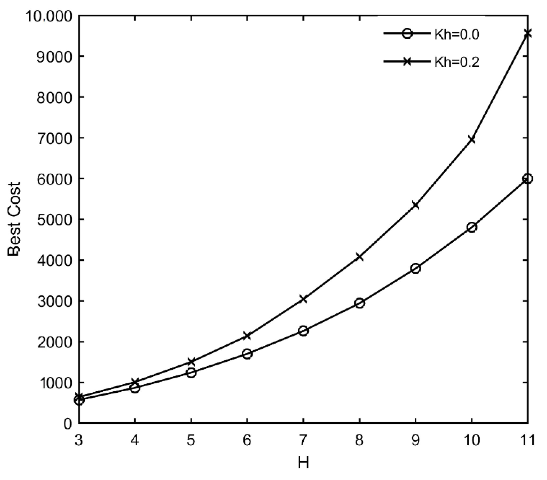
• The performance of the new algorithm for optimizing retaining structures subjected to both static and dynamic loading conditions indicates that the WEA design is nearly 5% less expensive than the previous approach;
• The numerical investigations show that, when compared to the other techniques, the newly proposed algorithm for the optimization of retaining structures is quite reliable and effective;
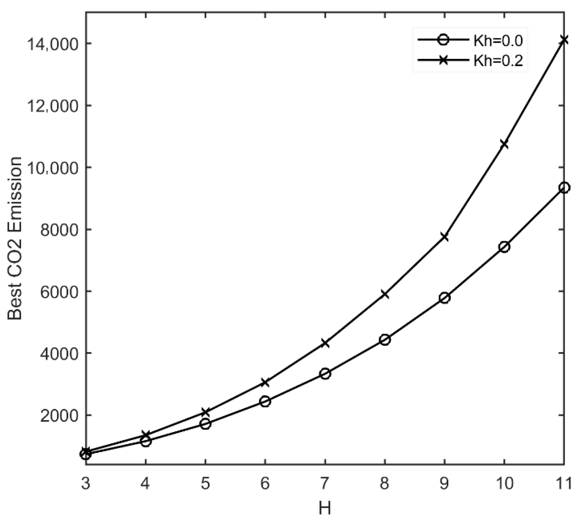
• Finally, seismic optimization results reveal that by increasing the horizontal acceleration coefficient to 0.2, the best cost and best CO₂ emission designs will be increased by up to 12% and 11.1%, respectively.

In future research, the binary version of the WEA can be developed to handle discontinuous problems. In addition, it is expected to develop the multi-objective WEA. Moreover, the WEA may also be applied to address several optimization issues in various fields, including feature selection, neural networks, structural optimization, photovoltaic models, power system stabilization, big data applications, and so on.

References

1. Holland, J.H. Genetic algorithms. Sci. Am. 1992, 267, 66–73. [Google Scholar] [CrossRef]
2. Dorigo, M.; Di Caro, G. Ant colony optimization: A new meta-heuristic. In Proceedings of the 1999 Congress on Evolutionary Computation—CEC99 (Cat. No. 99TH8406), Washington, DC, USA, 6–9 July 1999; pp. 1470–1477. [Google Scholar]
3. Kennedy, J.; Eberhart, R. Particle swarm optimization. In Proceedings of the ICNN’95—International Conference on Neural Networks, Perth, WA, Australia, 27 November–1 December 1995; pp. 1942–1948. [Google Scholar]
4. Cheng, Y.M.; Li, L.; Chi, S.-C.; Wei, W. Particle swarm optimization algorithm for the location of the critical non-circular failure surface in two-dimensional slope stability analysis. Comput. Geotech. 2007, 34, 92–103. [Google Scholar] [CrossRef]
5. Zolfaghari, A.R.; Heath, A.C.; McCombie, P.F. Simple genetic algorithm search for critical non-circular failure surface in slope stability analysis. Comput. Geotech. 2005, 32, 139–152. [Google Scholar] [CrossRef]
6. Angelo, J.S.; Bernardino, H.S.; Barbosa, H.J. Ant colony approaches for multiobjective structural optimization problems with a cardinality constraint. Adv. Eng. Softw. 2015, 80, 101–115. [Google Scholar] [CrossRef]
7. Khajehzadeh, M.; Keawsawasvong, S.; Sarir, P.; Khailany, D.K. Seismic Analysis of Earth Slope Using a Novel Sequential Hybrid Optimization Algorithm. Period. Polytech. Civ. Eng. 2022, 66, 355–366. [Google Scholar] [CrossRef]
8. Li, S.; Gong, W.; Gu, Q. A comprehensive survey on meta-heuristic algorithms for parameter extraction of photovoltaic models. Renew. Sustain. Energy Rev. 2021, 141, 110828. [Google Scholar] [CrossRef]
9. Boussaïd, I.; Lepagnot, J.; Siarry, P. A survey on optimization metaheuristics. Inf. Sci. 2013, 237, 82–117. [Google Scholar] [CrossRef]
10. Wolpert, D.H.; Macready, W.G. No free lunch theorems for optimization. IEEE Trans. Evol. Comput. 1997, 1, 67–82. [Google Scholar] [CrossRef]
11. Catalonia Institute of Construction Technology. BEDEC PR/PCT ITEC Material Database; Catalonia Institute of Construction Technology: Barcelona, Spain, 2016. [Google Scholar]
12. Yepes, V.; Gonzalez-Vidosa, F.; Alcala, J.; Villalba, P. CO2-optimization design of reinforced concrete retaining walls based on a VNS-threshold acceptance strategy. J. Comput. Civ. Eng. 2012, 26, 378–386. [Google Scholar] [CrossRef]
13. Worrell, E.; Price, L.; Martin, N.; Hendriks, C.; Meida, L.O. Carbon dioxide emissions from the global cement industry. Annu. Rev. Energy Environ. 2001, 26, 303–329. [Google Scholar] [CrossRef]
14. Paya-Zaforteza, I.; Yepes, V.; Hospitaler, A.; Gonzalez-Vidosa, F. CO2-optimization of reinforced concrete frames by simulated annealing. Eng. Struct. 2009, 31, 1501–1508. [Google Scholar] [CrossRef]
15. Nelson, D.P. Cost and CO2 Optimization of Reinforced Concrete Beams using a Big Bang-Big Crunch Algorithm. Master’s Thesis, University of Memphis, Memphis, TN, USA, 2014. [Google Scholar]
16. Camp, C.V.; Assadollahi, A. CO2and cost optimization of reinforced concrete footings using a hybrid big bang-big crunch algorithm. Struct. Multidiscip. Optim. 2013, 48, 411–426. [Google Scholar] [CrossRef]
17. Yepes, V.; Martí, J.V.; García-Segura, T. Cost and CO2 emission optimization of precast–prestressed concrete U-beam road bridges by a hybrid glowworm swarm algorithm. Autom. Constr. 2015, 49, 123–134. [Google Scholar] [CrossRef]
18. Beni, G.; Wang, J. Swarm intelligence in cellular robotic systems. In Robots and Biological Systems: Towards a New Bionics? Springer: Berlin/Heidelberg, Germany, 1993; pp. 703–712. [Google Scholar]
19. Zhang, J.-R.; Zhang, J.; Lok, T.-M.; Lyu, M.R. A hybrid particle swarm optimization–back-propagation algorithm for feedforward neural network training. Appl. Math. Comput. 2007, 185, 1026–1037. [Google Scholar] [CrossRef]
20. Khajehzadeh, M.; Taha, M.R.; El-Shafie, A.; Eslami, M. Modified particle swarm optimization for optimum design of spread footing and retaining wall. J. Zhejiang Univ.-Sci. A 2011, 12, 415–427. [Google Scholar] [CrossRef]
21. Montalvo, I.; Izquierdo, J.; Pérez, R.; Tung, M.M. Particle swarm optimization applied to the design of water supply systems. Comput. Math. Appl. 2008, 56, 769–776. [Google Scholar] [CrossRef]
22. Eslami, M.; Shareef, H.; Mohamed, A. Optimization and coordination of damping controls for optimal oscillations damping in multi-machine power system. Int. Rev. Electr. Eng. (IREE) 2011, 6, 1984–1993. [Google Scholar]
23. Eslami, M.; Shareef, H.; Mohamed, A.; Khajehzadeh, M. Particle swarm optimization for simultaneous tuning of static var compensator and power system stabilizer. Przegląd Elektrotech. (Electr. Rev.) 2011, 87, 343–347. [Google Scholar]
24. Liu, W.; Wang, Z.; Liu, X.; Zeng, N.; Bell, D. A novel particle swarm optimization approach for patient clustering from emergency departments. IEEE Trans. Evol. Comput. 2018, 23, 632–644. [Google Scholar] [CrossRef]
25. Kahatadeniya, K.S.; Nanakorn, P.; Neaupane, K.M. Determination of the critical failure surface for slope stability analysis using ant colony optimization. Eng. Geol. 2009, 108, 133–141. [Google Scholar] [CrossRef]
26. Xu, C.; Gordan, B.; Koopialipoor, M.; Armaghani, D.J.; Tahir, M.; Zhang, X. Improving performance of retaining walls under dynamic conditions developing an optimized ANN based on ant colony optimization technique. IEEE Access 2019, 7, 94692–94700. [Google Scholar] [CrossRef]
27. Gao, W. Modified ant colony optimization with improved tour construction and pheromone updating strategies for traveling salesman problem. Soft Comput. 2021, 25, 3263–3289. [Google Scholar] [CrossRef]
28. Karaboga, D.; Basturk, B. Artificial bee colony (ABC) optimization algorithm for solving constrained optimization problems. In Proceedings of the International Fuzzy Systems Association World Congress, Cancun, Mexico, 18–21 June 2007; pp. 789–798. [Google Scholar]
29. Ozturk, H.T.; Durmus, A. Optimum cost design of RC columns using artificial bee colony algorithm. Struct. Eng. Mech. Int. J. 2013, 45, 643–654. [Google Scholar] [CrossRef]
30. Akay, B.; Karaboga, D. Artificial bee colony algorithm for large-scale problems and engineering design optimization. J. Intell. Manuf. 2012, 23, 1001–1014. [Google Scholar] [CrossRef]
31. Habib, H.U.R.; Subramaniam, U.; Waqar, A.; Farhan, B.S.; Kotb, K.M.; Wang, S. Energy cost optimization of hybrid renewables based V2G microgrid considering multi objective function by using artificial bee colony optimization. IEEE Access 2020, 8, 62076–62093. [Google Scholar] [CrossRef]
32. Yang, X.S. Firefly algorithms for multimodal optimization. Lect. Notes Comput. Sci. 2009, 5792, 169–178. [Google Scholar]
33. Khajehzadeh, M.; Taha, M.R.; Eslami, M. Opposition-based firefly algorithm for earth slope stability evaluation. China Ocean Eng. 2014, 28, 713–724. [Google Scholar] [CrossRef]
34. Apostolopoulos, T.; Vlachos, A. Application of the firefly algorithm for solving the economic emissions load dispatch problem. Int. J. Comb. 2011, 2011, 523806. [Google Scholar] [CrossRef]
35. Khurshaid, T.; Wadood, A.; Farkoush, S.G.; Kim, C.-H.; Yu, J.; Rhee, S.-B. Improved firefly algorithm for the optimal coordination of directional overcurrent relays. IEEE Access 2019, 7, 78503–78514. [Google Scholar] [CrossRef]
36. Gandomi, A.H.; Alavi, A.H. Krill herd: A new bio-inspired optimization algorithm. Commun. Nonlinear Sci. Numer. Simul. 2012, 17, 4831–4845. [Google Scholar] [CrossRef]
37. Askarzadeh, A. A novel metaheuristic method for solving constrained engineering optimization problems: Crow search algorithm. Comput. Struct. 2016, 169, 1–12. [Google Scholar] [CrossRef]
38. Dhiman, G.; Garg, M.; Nagar, A.; Kumar, V.; Dehghani, M. A novel algorithm for global optimization: Rat swarm optimizer. J. Ambient Intell. Humaniz. Comput. 2020, 12, 8457–8482. [Google Scholar] [CrossRef]
39. Khajehzadeh, M.; Keawsawasvong, S.; Nehdi, M.L. Effective hybrid soft computing approach for optimum design of shallow foundations. Sustainability 2022, 14, 1847. [Google Scholar] [CrossRef]
40. Shehadeh, H.A.; Ahmedy, I.; Idris, M.Y.I. Sperm swarm optimization algorithm for optimizing wireless sensor network challenges. In Proceedings of the 6th International Conference on Communications and Broadband Networking, Singapore, 24–26 February 2018; pp. 53–59. [Google Scholar]
41. Khajehzadeh, M.; Kalhor, A.; Tehrani, M.S.; Jebeli, M. Optimum design of retaining structures under seismic loading using adaptive sperm swarm optimization. Struct. Eng. Mech. 2022, 81, 93–102. [Google Scholar]
42. Braik, M.S. Chameleon Swarm Algorithm: A bio-inspired optimizer for solving engineering design problems. Expert Syst. Appl. 2021, 174, 114685. [Google Scholar] [CrossRef]
43. Fernandes, F.; Sousa, T.; Silva, M.; Morais, H.; Vale, Z.; Faria, P. Genetic algorithm methodology applied to intelligent house control. In Proceedings of the 2011 IEEE Symposium on Computational Intelligence Applications In Smart Grid (CIASG), Paris, France, 11–15 April 2011; pp. 1–8. [Google Scholar]
44. Eslami, M.; Shareef, H.; Mohamed, A.; Khajehzadeh, M. Damping Controller Design for Power System Oscillations Using Hybrid GA-SQP. Int. Rev. Electr. Eng.-IREE 2011, 6, 888–896. [Google Scholar]
45. Johnson, F.; Valderrama, A.; Valle, C.; Crawford, B.; Soto, R.; Ñanculef, R. Automating configuration of convolutional neural network hyperparameters using genetic algorithm. IEEE Access 2020, 8, 156139–156152. [Google Scholar] [CrossRef]
46. Storn, R.; Price, K. Differential evolution a simple evolution strategy for fast optimization. Dr. Dobb’s J. 1997, 22, 18–24. [Google Scholar]
47. Ilonen, J.; Kamarainen, J.-K.; Lampinen, J. Differential evolution training algorithm for feed-forward neural networks. Neural Process. Lett. 2003, 17, 93–105. [Google Scholar] [CrossRef]
48. Goudos, S.K.; Siakavara, K.; Samaras, T.; Vafiadis, E.E.; Sahalos, J.N. Self-adaptive differential evolution applied to real-valued antenna and microwave design problems. IEEE Trans. Antennas Propag. 2011, 59, 1286–1298. [Google Scholar] [CrossRef]
49. Maučec, M.S.; Brest, J.; Bošković, B. Improved differential evolution for large-scale black-box optimization. IEEE Access 2018, 6, 29516–29531. [Google Scholar] [CrossRef]
50. Huang, X.; Xie, Y. Bidirectional evolutionary topology optimization for structures with geometrical and material nonlinearities. AIAA J. 2007, 45, 308–313. [Google Scholar] [CrossRef]
51. Rad, M.M.; Ibrahim, S.K. Optimal plastic analysis and design of pile foundations under reliable conditions. Period. Polytech. Civ. Eng. 2021, 65, 761–767. [Google Scholar]
52. Rad, M.M.; Habashneh, M.; Logo, J. Elasto-Plastic limit analysis of reliability based geometrically nonlinear bi-directional evolutionary topology optimization. In Structures; Elsevier: Amsterdam, The Netherlands, 2021; pp. 1720–1733. [Google Scholar]
53. Habashneh, M.; Movahedi Rad, M. Reliability based geometrically nonlinear bi-directional evolutionary structural optimization of elasto-plastic material. Sci. Rep. 2022, 12, 5989. [Google Scholar] [CrossRef]
54. Simon, D. Biogeography-based optimization. IEEE Trans. Evol. Comput. 2008, 12, 702–713. [Google Scholar] [CrossRef]
55. Abd Elaziz, M.; Lu, S.; He, S. A multi-leader whale optimization algorithm for global optimization and image segmentation. Expert Syst. Appl. 2021, 175, 114841. [Google Scholar] [CrossRef]
56. Jaderyan, M.; Khotanlou, H. Virulence optimization algorithm. Appl. Soft Comput. 2016, 43, 596–618. [Google Scholar] [CrossRef]
57. Erol, O.K.; Eksin, I. A new optimization method: Big bang–big crunch. Adv. Eng. Softw. 2006, 37, 106–111. [Google Scholar] [CrossRef]
58. Camp, C.V.; Akin, A. Design of retaining walls using big bang–big crunch optimization. J. Struct. Eng. 2012, 138, 438–448. [Google Scholar] [CrossRef]
59. Sedighizadeh, M.; Esmaili, M.; Eisapour-Moarref, A. Voltage and frequency regulation in autonomous microgrids using Hybrid Big Bang-Big Crunch algorithm. Appl. Soft Comput. 2017, 52, 176–189. [Google Scholar] [CrossRef]
60. Prayogo, D.; Cheng, M.-Y.; Wu, Y.-W.; Herdany, A.A.; Prayogo, H. Differential Big Bang-Big Crunch algorithm for construction-engineering design optimization. Autom. Constr. 2018, 85, 290–304. [Google Scholar] [CrossRef]
61. Rashedi, E.; Nezamabadi-pour, H.; Saryazdi, S. GSA: A gravitational search algorithm. Inf. Sci. 2009, 179, 2232–2248. [Google Scholar] [CrossRef]
62. Khajehzadeh, M.; Taha, M.R.; Eslami, M. Multi-objective optimization of foundation using global-local gravitational search algorithm. Struct. Eng. Mech.Int. J. 2014, 50, 257–273. [Google Scholar] [CrossRef]
63. Khajehzadeh, M.; Taha, M.R.; Eslami, M. Multi-objective optimisation of retaining walls using hybrid adaptive gravitational search algorithm. Civ. Eng. Environ. Syst. 2014, 31, 229–242. [Google Scholar] [CrossRef]
64. Rashedi, E.; Nezamabadi-Pour, H.; Saryazdi, S. Filter modeling using gravitational search algorithm. Eng. Appl. Artif. Intell. 2011, 24, 117–122. [Google Scholar] [CrossRef]
65. Zhu, L.; He, S.; Wang, L.; Zeng, W.; Yang, J. Feature selection using an improved gravitational search algorithm. IEEE Access 2019, 7, 114440–114448. [Google Scholar] [CrossRef]
66. Formato, R.A. Central force optimization: A new nature inspired computational framework for multidimensional search and optimization. In Nature Inspired Cooperative Strategies for Optimization (NICSO 2007); Springer: Berlin/Heidelberg, Germany, 2008; pp. 221–238. [Google Scholar]
67. Hatamlou, A. Black hole: A new heuristic optimization approach for data clustering. Inf. Sci. 2013, 222, 175–184. [Google Scholar] [CrossRef]
68. Moghaddam, F.F.; Moghaddam, R.F.; Cheriet, M. Curved space optimization: A random search based on general relativity theory. arXiv 2012, arXiv:1208.2214. [Google Scholar]
69. Kaveh, A.; Khayatazad, M. A new meta-heuristic method: Ray optimization. Comput. Struct. 2012, 112, 283–294. [Google Scholar] [CrossRef]
70. Mirjalili, S.; Mirjalili, S.M.; Hatamlou, A. Multi-verse optimizer: A nature-inspired algorithm for global optimization. Neural Comput. Appl. 2016, 27, 495–513. [Google Scholar] [CrossRef]
71. Rao, R.V. Teaching-learning-based optimization algorithm. In Teaching Learning Based Optimization Algorithm; Springer: Berlin/Heidelberg, Germany, 2016; pp. 9–39. [Google Scholar]
72. Rao, R.V.; Savsani, V.J.; Vakharia, D. Teaching–learning-based optimization: A novel method for constrained mechanical design optimization problems. Comput.-Aided Des. 2011, 43, 303–315. [Google Scholar] [CrossRef]
73. Dede, T.; Togan, V. A teaching learning based optimization for truss structures with frequency constraints. Struct. Eng. Mech.Int. J. 2015, 53, 833–845. [Google Scholar] [CrossRef]
74. Kumar, M.; Kulkarni, A.J.; Satapathy, S.C. Socio evolution & learning optimization algorithm: A socio-inspired optimization methodology. Future Gener. Comput. Syst. 2018, 81, 252–272. [Google Scholar]
75. Atashpaz-Gargari, E.; Lucas, C. Imperialist competitive algorithm: An algorithm for optimization inspired by imperialistic competition. In Proceedings of the 2007 IEEE Congress on Evolutionary Computation, Singapore, 25–28 September 2007; pp. 4661–4667. [Google Scholar]
76. Ghorbani, N.; Babaei, E. Exchange market algorithm. Appl. Soft Comput. 2014, 19, 177–187. [Google Scholar] [CrossRef]
77. Moghdani, R.; Salimifard, K. Volleyball premier league algorithm. Appl. Soft Comput. 2018, 64, 161–185. [Google Scholar] [CrossRef]
78. Uymaz, S.A.; Tezel, G.; Yel, E. Artificial algae algorithm (AAA) for nonlinear global optimization. Appl. Soft Comput. 2015, 31, 153–171. [Google Scholar] [CrossRef]
79. Evans, R.J.; Wilson, J.D.; Amar, A.; Douse, A.; MacLennan, A.; Ratcliffe, N.; Whitfield, D.P. Growth and demography of a re-introduced population of White-tailed Eagles Haliaeetus albicilla. Ibis 2009, 151, 244–254. [Google Scholar] [CrossRef]
80. Nadjafzadeh, M.; Hofer, H.; Krone, O. The link between feeding ecology and lead poisoning in white-tailed eagles. J. Wildl. Manag. 2013, 77, 48–57. [Google Scholar] [CrossRef]
81. Nadjafzadeh, M.; Hofer, H.; Krone, O. Sit-and-wait for large prey: Foraging strategy and prey choice of White-tailed Eagles. J. Ornithol. 2016, 157, 165–178. [Google Scholar] [CrossRef]
82. Olorunda, O.; Engelbrecht, A.P. Measuring exploration/exploitation in particle swarms using swarm diversity. In Proceedings of the 2008 IEEE congress on evolutionary computation (IEEE world congress on computational intelligence), Hong Kong, China, 1–6 June 2008; pp. 1128–1134. [Google Scholar]
83. Patel, V.K.; Savsani, V.J. Heat transfer search (HTS): A novel optimization algorithm. Inf. Sci. 2015, 324, 217–246. [Google Scholar] [CrossRef]
84. Digalakis, J.G.; Margaritis, K.G. On benchmarking functions for genetic algorithms. Int. J. Comput. Math. 2001, 77, 481–506. [Google Scholar] [CrossRef]
85. Hussain, K.; Salleh, M.N.M.; Cheng, S.; Naseem, R. Common benchmark functions for metaheuristic evaluation: A review. JOIV Int. J. Inform. Vis. 2017, 1, 218–223. [Google Scholar] [CrossRef]
86. Askari, Q.; Younas, I.; Saeed, M. Political Optimizer: A novel socio-inspired meta-heuristic for global optimization. Knowl. -Based Syst. 2020, 195, 105709. [Google Scholar] [CrossRef]
87. Mirjalili, S.; Mirjalili, S.M.; Lewis, A. Grey wolf optimizer. Adv. Eng. Softw. 2014, 69, 46–61. [Google Scholar] [CrossRef]
88. Das, B.M.; Luo, Z. Principles of Soil Dynamics; Cengage Learning: Boston, MA, USA, 2016. [Google Scholar]
89. ACI Committee. Building Code Requirements for Structural Concrete (ACI 318-05); American Concrete Institute: Farmington Hills, MI, USA, 2005. [Google Scholar]
90. Das, B.M.; Sobhan, K. Principles of Geotechnical Engineering, USA; Brooks/Cole-Thomson Learning Inc: Boston, MA, USA, 2002. [Google Scholar]
91. Gandomi, A.; Kashani, A.; Zeighami, F. Retaining wall optimization using interior search algorithm with different bound constraint handling. Int. J. Numer. Anal. Methods Geomech. 2017, 41, 1304–1331. [Google Scholar] [CrossRef]
Figure 1. The WEA flowchart.
Sustainability 14 10673 g001
Figure 2. 3-D view of unimodal test problems.
Sustainability 14 10673 g002aSustainability 14 10673 g002b
Figure 3. 3-D view of multimodal test problems.
Sustainability 14 10673 g003aSustainability 14 10673 g003b
Figure 4. Convergence progress of considered algorithms.
Sustainability 14 10673 g004aSustainability 14 10673 g004bSustainability 14 10673 g004c
Figure 5. Retaining structure cross section.
Sustainability 14 10673 g005
Figure 6. Effect of height of the wall and Kh on low-cost design.
Sustainability 14 10673 g006
Figure 7. Effect of height of the wall and Kh on low-CO2 emission design.
Sustainability 14 10673 g007
Figure 8. Effects of friction angle on low-cost designs (H = 3 m).
Sustainability 14 10673 g008
Figure 9. Effects of friction angle on low- CO2 emission designs (H = 3 m).
Sustainability 14 10673 g009
Figure 10. Effects of friction angle on low-cost designs (H = 6 m).
Sustainability 14 10673 g010
Figure 11. Effects of friction angle on low-CO2 emission designs (H = 6 m).
Sustainability 14 10673 g011