Evaluation of Air Pollutants in Extra-Long Road Tunnel with the Combination of Pollutants Nonlinear Evolution and Machine Learning Method
Abstract
:1. Introduction
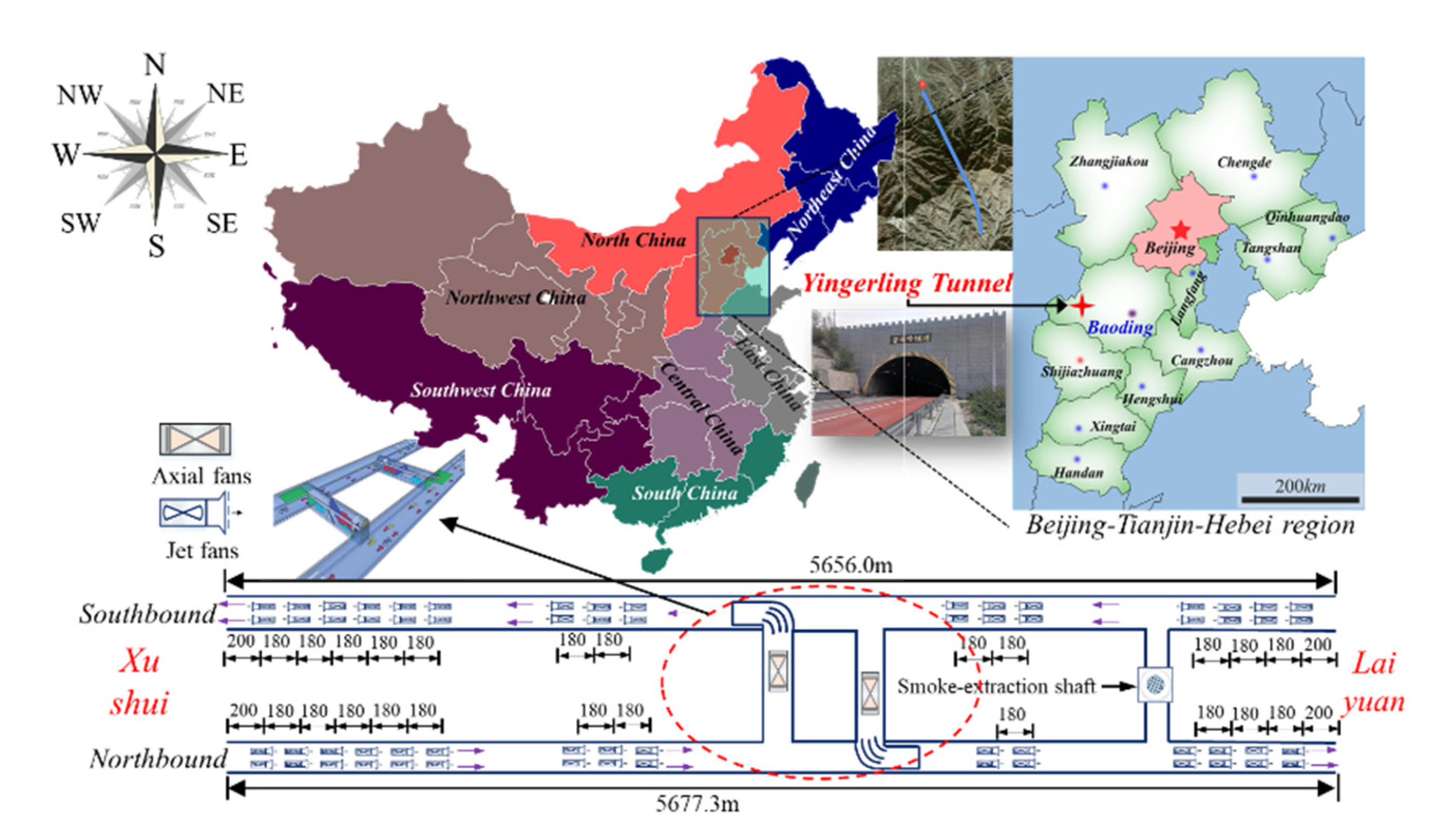
2. Tunnel Description
3. Experimental Method
3.1. Traffic Data
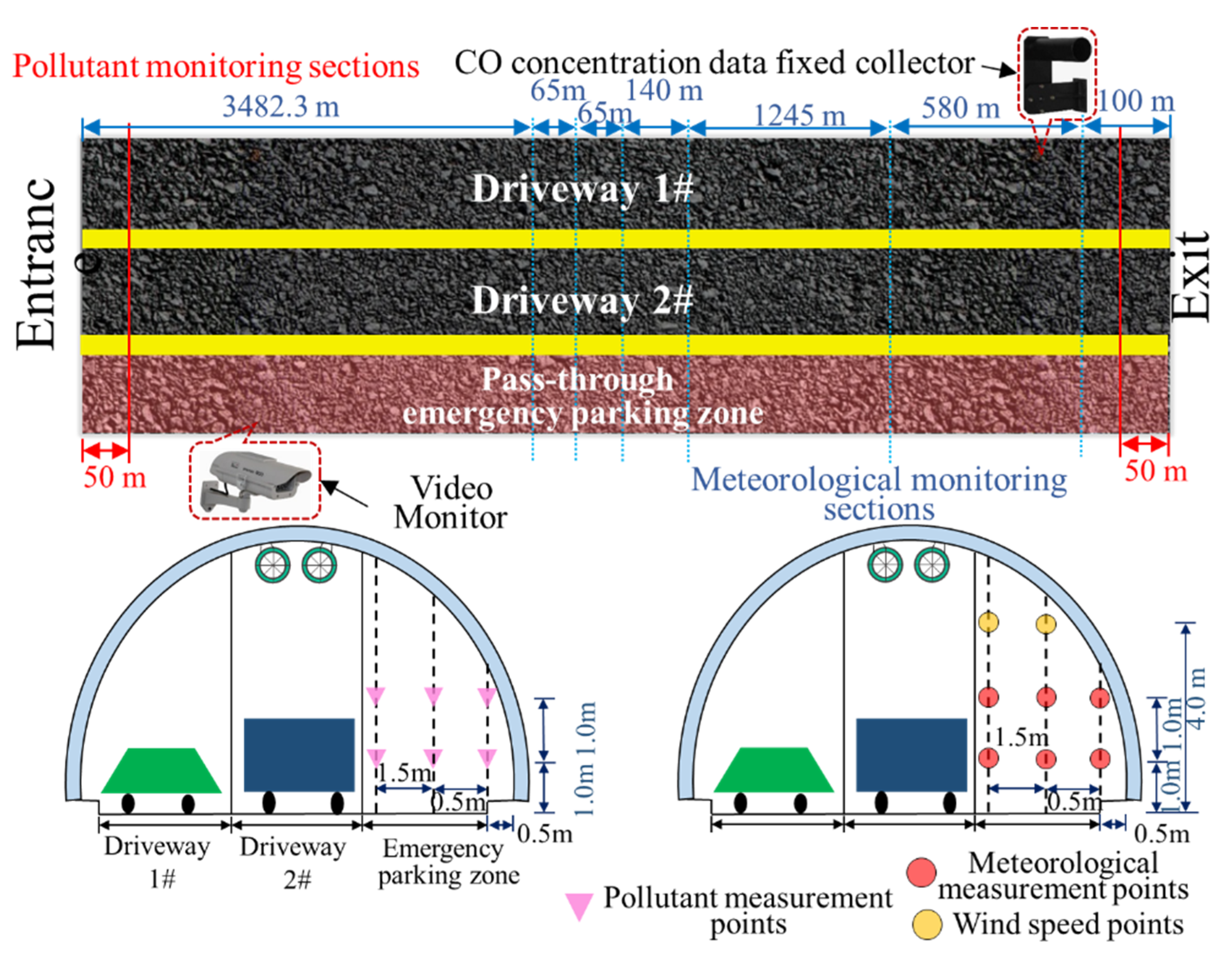
3.2. Environmental Parameters
3.3. Pollutant Concentration
4. Methodology
4.1. Multifractal Detrended Fluctuation Analysis Method (MFDFA)
- (1)
- For the pollutant concentration time series xt, t = 1, 2, 3, …, N, construct the cumulative deviation series Yi. The time series Yi is divided equidistantly into Ns intervals.
- (2)
- To obtain the mean square error F2(v, s), the local trend of the 2Ns subintervals is calculated by fitting each subinterval v (v = 1, 2, …, 2Ns) with the least-squares method. The yv(i) is the fitted polynomial for the v segment of data in Equation (2).
- (3)
- The fluctuation function Fq(s) of order q is calculated, as shown in Equation (3).>
- (4)
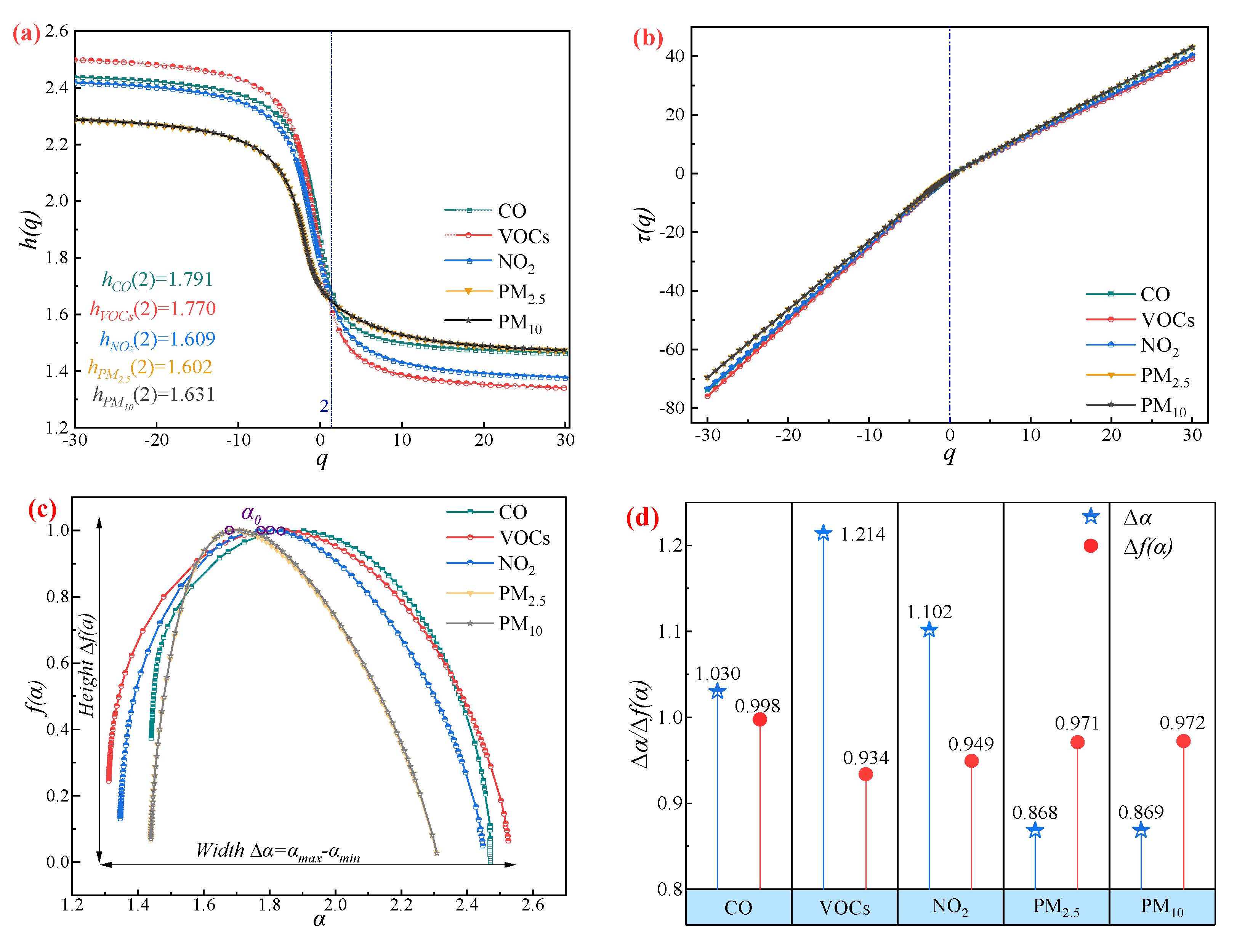
- The power-law relationship between the volatility function Fq(s) of order q and the time scale s holds when the time series xt has self-similarity, as shown in Equations (4) and (5).where: h(q) is the generalized Hurst exponent and defines. The mass index τ(q) and the fractal dimension D(q) in multifractal theory satisfy the Equation (6).
4.2. Random Forest Model (RF)
5. Results and Discussion
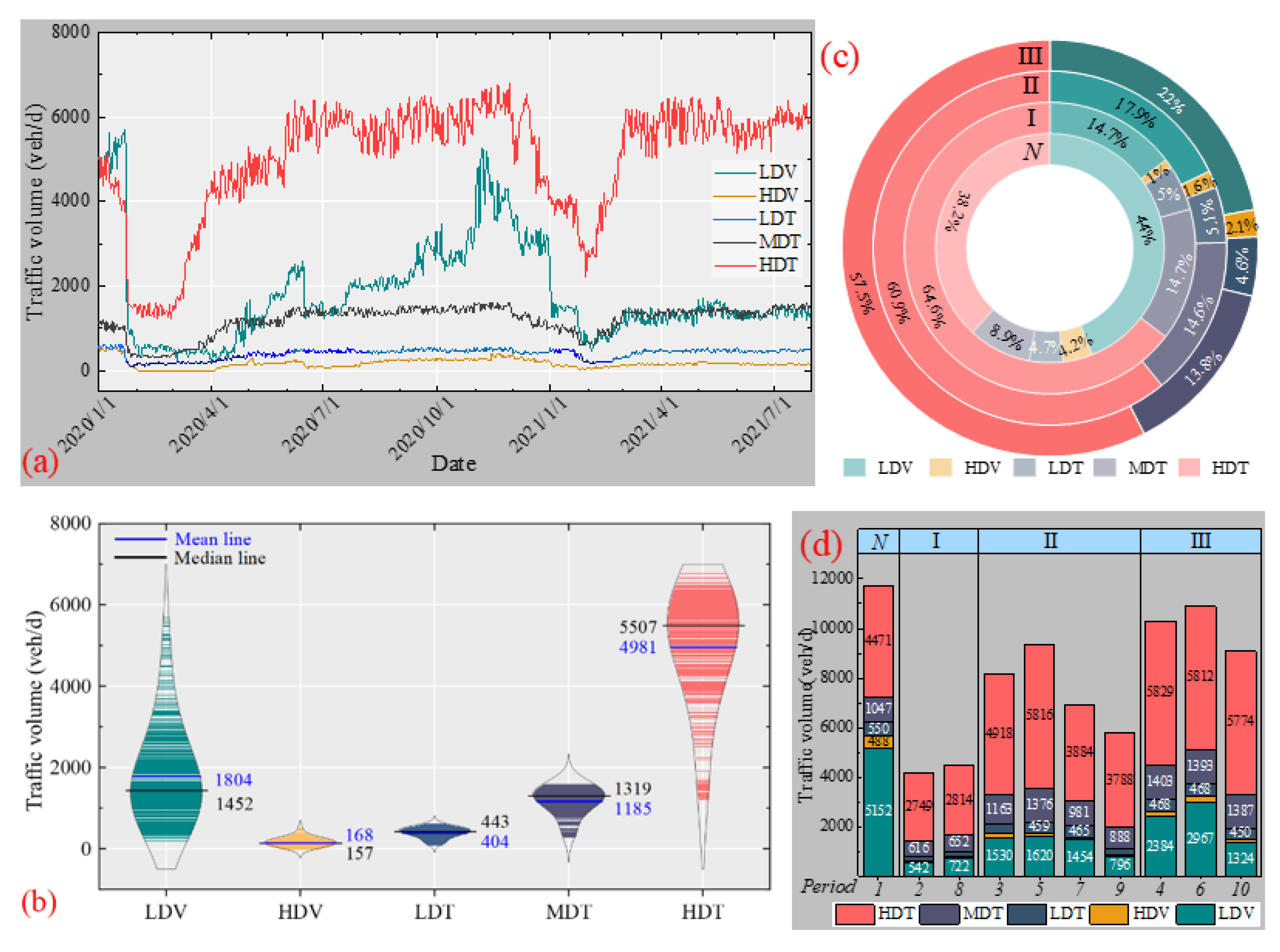
5.1. Traffic Characteristic
5.2. Monitoring Results
5.2.1. Pollutant Concentrations
5.2.2. Tunnel Environment Parameters
5.3. Relationship between Pollutant Concentrations and Environmental Parameters
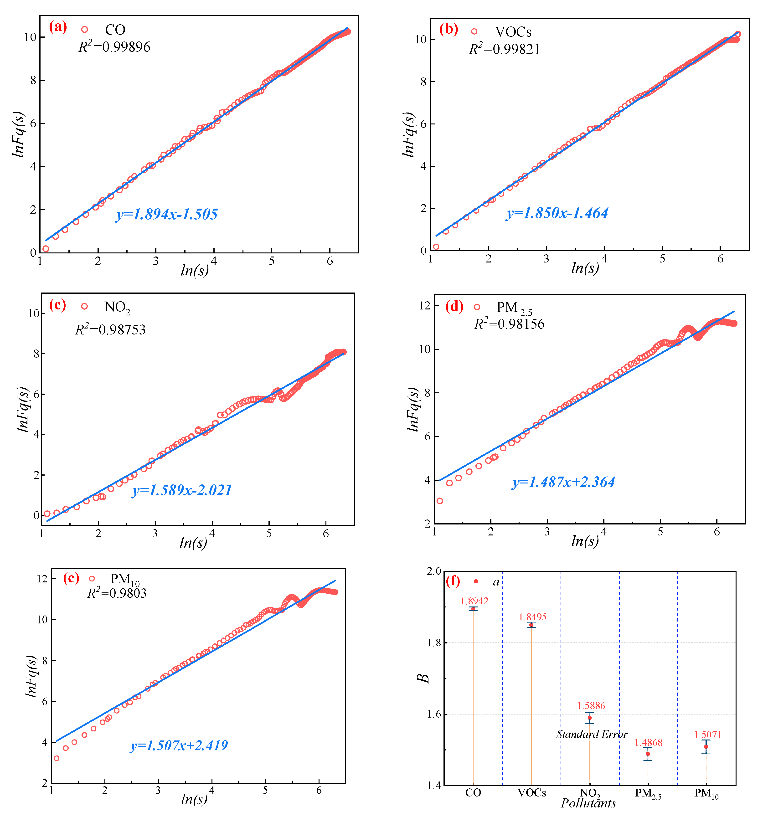
5.4. Pollutants’ Nonlinear Evolution
5.5. Prediction of Air Pollutants in YEL Tunnel
6. Conclusions
- (1)
- Different epidemic control levels had different degrees of impact on daily traffic for different types of vehicles, with the HDT only showing a stronger response to level-I control. The same control level also had different effects on traffic flow in different periods.
- (2)
- The pollutant concentrations did not fluctuate significantly during the observation period. Typical correlation analysis results show wind speed largely influences pollutants concentration, ranging from −0.523 to 0.673. The correlations between aerosol pollutant concentrations and wind speed are negative, and the aerosol pollutants are more likely to be discharged from the tunnel. The traffic wind dilutes the pollutant concentrations, and the higher the traffic wind, the higher the pollutant emissions.
- (3)
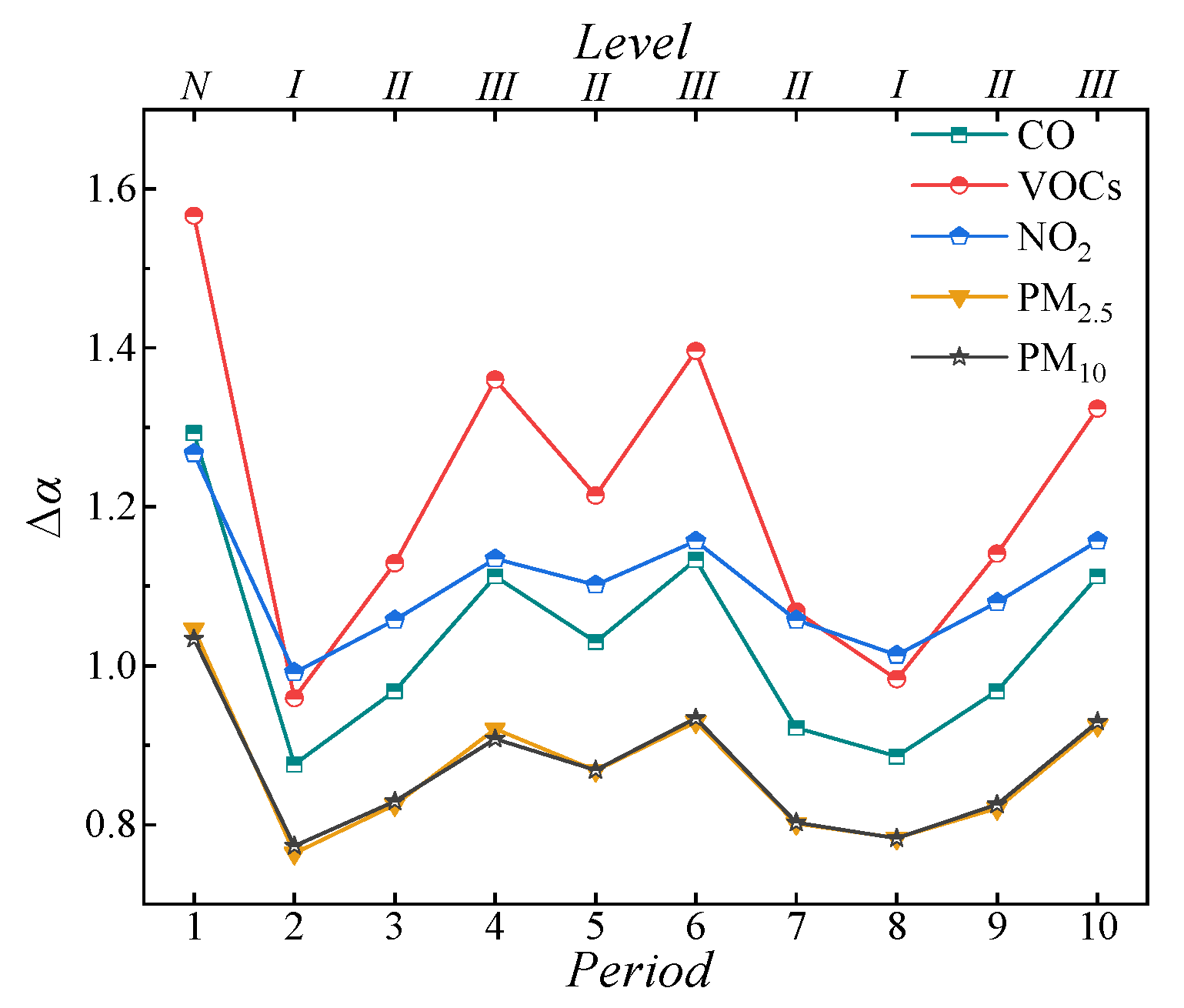
- The MFDFA results indicate that the pollutant concentrations inside the tunnel exhibit long-term persistence, with CO concentrations being the most significant (hco(2) = 1.791), and relatively weak for PM2.5 concentrations (hPM2.5(2) = 1.602). The evolution of each pollutant has a stable power-law distribution structure, and the pollutant evolution may have the Self-Organized Critical (SOC) state.
- (4)
- Through the validation results for the 10-Fold CV and different mathematical models, the created RF models demonstrated high prediction accuracy and generalization ability. The HDT traffic flow was the controlling factor for each pollutant (39.26 to 82.38%). The concentration inversion findings revealed that the prediction accuracy (R2) is 0.9942 for CO, 0.9825 for VOCs, 0.9903 for NO2, 0.9758 for PM2.5, and 0.9845 for PM10.
Author Contributions
Funding
Institutional Review Board Statement
Informed Consent Statement
Data Availability Statement
Acknowledgments
Conflicts of Interest
References
- Alves, C.A.; Vicente, A.M.; Rocha, S.; Vasconcellos, P. Hopanoid hydrocarbons in PM10 from road tunnels in So Paulo, Brazil. Air Qual. Atmos. Health 2017, 10, 799–807. [Google Scholar]
- Santos, E.M.; Azevedo, D.D. Impact on ground-level ozone formation by emission characterization of volatile organic compounds from a flex-fuel light-duty vehicle fleet in a traffic tunnel in Rio de Janeiro, Brazil. Air Qual. Atmos. Health 2021, 14, 259–270. [Google Scholar]
- Zhang, Z.Q.; Zhang, H.; Tan, Y.J.; Yang, H.Y. Natural wind utilization in the vertical shaft of a super-long highway tunnel and its energy saving effect. Build. Environ. 2018, 145, 140–152. [Google Scholar]
- Steffens, J.T.; Heist, D.K.; Perry, S.G.; Isakov, V.; Baldauf, R.W.; Zhang, K.M. Effects of roadway configurations on near-road air quality and the implications on roadway designs. Atmos. Environ. 2014, 94, 74–85. [Google Scholar]
- Yang, Q.H.; Shen, H.G.; Liang, Z. Analysis of particulate matter and carbon monoxide emission rates from vehicles in a Shanghai tunnel. Sustain. Cities Soc. 2020, 56, 102104. [Google Scholar]
- Ma, Z.L.; Chien, S.I.J.; Dong, C.J.; Hu, D.W.; Xu, T. Exploring factors affecting injury severity of crashes in freeway tunnels. Tunn. Undergr. Space Technol. 2016, 59, 100–104. [Google Scholar]
- Giunta, M. Assessment of the Impact of CO, NOx and PM10 on Air Quality during Road Construction and Operation Phases. Sustainability 2020, 12, 10549. [Google Scholar]
- Rada, E.C.; Magaril, E.R.; Schiavon, M.; Karaeva, A.; Chashchin, M.; Torretta, V. MSW Management in Universities: Sharing Best Practices. Sustainability 2020, 12, 5084. [Google Scholar]
- Torretta, V.; Tolkou, A.; Katsoyiannis, I.; Schiavon, M. Second-Hand Smoke Exposure Effects on Human Health: Evaluation of PM10 Concentrations in the External Areas of a University Campus. Sustainability 2020, 12, 2948. [Google Scholar]
- Rada, E.C.; Schiavon, M.; Torretta, V. A regulatory strategy for the emission control of hexavalent chromium from waste-to-energy plants. J. Clean Prod. 2021, 278, 123415. [Google Scholar]
- Klockner, P.; Seiwert, B.; Weyrauch, S.; Escher, B.I.; Reemtsma, T.; Wagner, S. Comprehensive characterization of tire and road wear particles in highway tunnel road dust by use of size and density fractionation. Chemosphere 2021, 279, 130530. [Google Scholar] [PubMed]
- Wang, R.Y.; Ye, X.N.; Liu, Y.X.; Li, H.W.; Yang, X.; Chen, J.M.; Gao, W.; Yin, Z. Characteristics of atmospheric ammonia and its relationship with vehicle emissions in a megacity in China. Atmos. Environ. 2018, 182, 97–104. [Google Scholar]
- Luo, Y.B.; Chen, J.X.; Liu, W.W.; Ji, Z.; Ji, X.; Shi, Z.; Yuan, J.P.; Li, Y. Pollutant concentration measurement and emission factor analysis of highway tunnel with mainly HGVs in mountainous area. Tunn. Undergr. Space Technol. 2020, 106, 103591. [Google Scholar]
- Shahne, M.Z.; Arhami, M.; Hosseini, V.; El Haddad, I. Particulate emissions of real-world light-duty gasoline vehicle fleet in Iran. Environ. Pollut. 2022, 292, 118303. [Google Scholar]
- Zhang, J.S.; Peng, J.F.; Song, C.B.; Ma, C.; Men, Z.Y.; Wu, J.H.; Wu, L.; Wang, T.; Zhang, X.F.; Tao, S.C.; et al. Vehicular non-exhaust particulate emissions in Chinese megacities: Source profiles, real-world emission factors, and inventories. Environ. Pollut. 2020, 266, 115268. [Google Scholar]
- Pant, P.; Baker, S.J.; Shukla, A.; Maikawa, C.; Pollitt, K.J.G.; Harrison, R.M. The PM10 fraction of road dust in the UK and India: Characterization, source profiles and oxidative potential. Sci. Total Environ. 2015, 530, 445–452. [Google Scholar]
- Song, C.B.; Ma, C.; Zhang, Y.J.; Wang, T.; Wu, L.; Wang, P.; Liu, Y.; Li, Q.; Zhang, J.S.; Dai, Q.L.; et al. Heavy-duty diesel vehicles dominate vehicle emissions in a tunnel study in northern China. Sci. Total Environ. 2018, 637, 431–442. [Google Scholar]
- Gao, P.P.; Zhao, Y.B.; Ni, H.G. Incidence of real-world automotive parent and halogenated PAH in urban atmosphere. Environ. Pollut. 2018, 237, 515–522. [Google Scholar]
- Wang, M.N.; Wang, X.; Yu, L.; Deng, T. Field measurements of the environmental parameter and pollutant dispersion in urban undersea road tunnel. Build. Environ. 2019, 149, 100–108. [Google Scholar]
- Wang, Y.Q.; Xu, S.S.; Ren, R.; Zhang, S.Z.; Ren, Z.D. Application of the twin-tube complementary ventilation system in large-slopping road tunnels in China. Int. J. Vent. 2020, 19, 63–82. [Google Scholar]
- Jathar, S.H.; Sharma, N.; Galang, A.; Vanderheyden, C.; Takhar, M.; Chan, A.W.H.; Pierce, J.R.; Volckens, J. Measuring and modeling the primary organic aerosol volatility from a modern non-road diesel engine. Atmos. Environ. 2020, 223, 117221. [Google Scholar]
- Colella, F.; Rein, G.; Borchiellini, R.; Carvel, R.; Torero, J.L.; Verda, V. Calculation and design of tunnel ventilation systems using a two-scale modelling approach. Build. Environ. 2009, 44, 2357–2367. [Google Scholar]
- Lee, S.R.; Ryou, H.S. A numerical study on smoke movement in longitudinal ventilation tunnel fires for different aspect ratio. Build. Environ. 2006, 41, 719–725. [Google Scholar]
- Yang, D.; Huo, R.; Zhang, X.; Zhu, S.; Zhao, X. Comparative study on carbon monoxide stratification and thermal stratification in a horizontal channel fire. Build. Environ. 2012, 49, 1–8. [Google Scholar]
- Kam, W.; Liacos, J.W.; Schauer, J.J.; Delfino, R.J.; Sioutas, C. On-road emission factors of PM pollutants for light-duty vehicles (LDVs) based on urban street driving conditions. Atmos. Environ. 2012, 61, 378–386. [Google Scholar]
- Jiang, X.P.; Chen, X.G.; Xiao, N.Q.; Liao, X.J.; Fan, C.G. Influence of the competitive effect of V-shaped slope tunnel on smoke characteristics. Tunn. Undergr. Space Technol. 2021, 118, 104193. [Google Scholar]
- Savalanpour, H.; Farhanieh, B.; Afshin, H. Proposing a general formula to calculate the critical velocities in tunnels with different cross-sectional shapes. Tunn. Undergr. Space Technol. 2021, 110, 103798. [Google Scholar]
- Mukhtar, A.; Yusoff, M.Z.; Ng, K.C. The potential influence of building optimization and passive design strategies on natural ventilation systems in underground buildings: The state of the art. Tunn. Undergr. Space Technol. 2019, 92, 103065. [Google Scholar]
- Bhautmage, U.; Gokhale, S. Effects of moving-vehicle wakes on pollutant dispersion inside a highway road tunnel. Environ. Pollut. 2016, 218, 783–793. [Google Scholar]
- Wang, F.; Wang, M.; Wang, Q. Numerical study of effects of deflected angles of jet fans on the normal ventilation in a curved tunnel. Tunn. Undergr. Space Technol. 2012, 31, 80–85. [Google Scholar]
- Gokce, H.B.; Arioglu, E.; Copty, N.K.; Onay, T.T.; Gun, B. Exterior air quality monitoring for the Eurasia Tunnel in Istanbul, Turkey. Sci. Total Environ. 2020, 699, 134312. [Google Scholar] [CrossRef] [PubMed]
- Paull, N.J.; Irga, P.J.; Torpy, F.R. Active green wall plant health tolerance to diesel smoke exposure. Environ. Pollut. 2018, 240, 448–456. [Google Scholar] [PubMed]
- Baldauf, R. Roadside vegetation design characteristics that can improve local, near-road air quality. Transp. Res. Part D-Transp. Environ. 2017, 52, 354–361. [Google Scholar] [CrossRef] [PubMed]
- Dallmann, T.R.; DeMartini, S.J.; Kirchstetter, T.W.; Herndon, S.C.; Onasch, T.B.; Wood, E.C.; Harley, R.A. On-Road Measurement of Gas and Particle Phase Pollutant Emission Factors for Individual Heavy-Duty Diesel Trucks. Environ. Sci. Technol. 2012, 46, 8511–8518. [Google Scholar] [CrossRef] [PubMed]
- Song, X.C.; Zhao, Y. Numerical investigation of airflow patterns and pollutant dispersions induced by a fleet of vehicles inside road tunnels using dynamic mesh Part II: Pollutant dispersion and exposure levels. Atmos. Environ. 2019, 210, 198–210. [Google Scholar]
- Li, Q.; Chen, C. Survey and measurement of the vehicle pollutant emission in urban underground bifurcate tunnel, China. Sustain. Cities Soc. 2019, 48, 101519. [Google Scholar] [CrossRef]
- Li, H.C.; Chen, K.S.; Lai, C.H.; Wang, H.K. Measurements of Gaseous Pollutant Concentrations in the Hsuehshan Traffic Tunnel of Northern Taiwan. Aerosol Air Qual. Res. 2011, 11, 776–782. [Google Scholar] [CrossRef]
- Ma, C.M.; Hong, G.B.; Chang, C.T. Influence of Traffic Flow Patterns on Air Quality inside the Longest Tunnel in Asia. Aerosol Air Qual. Res. 2011, 11, 44–50. [Google Scholar]
- Chang, S.-C.; Lin, T.-H.; Lee, C.-T. On-road emission factors from light-duty vehicles measured in Hsuehshan Tunnel (12.9 km), the longest tunnel in Asia. Environ. Monit. Assess. 2009, 153, 187–200. [Google Scholar]
- Xu, H.M.; Feng, R.; Wang, Z.X.; Zhang, N.N.; Zhang, R.J.; He, K.L.; Wang, Q.Y.; Zhang, Q.; Sun, J.; Zhang, B.; et al. Environmental and health risks of VOCs in the longest inner-city tunnel in Xi’an, Northwest China: Implication of impact from new energy vehicles. Environ. Pollut. 2021, 282, 117057. [Google Scholar] [CrossRef]
- Hou, C.; Shao, L.Y.; Hu, W.; Zhang, D.Z.; Zhao, C.M.; Xing, J.P.; Huang, X.F.; Hu, M. Characteristics and aging of traffic-derived particles in a highway tunnel at a coastal city in southern China. Sci. Total Environ. 2018, 619, 1385–1393. [Google Scholar] [CrossRef] [PubMed]
- Dallmann, T.R.; Kirchstetter, T.W.; DeMartini, S.J.; Harley, R.A. Quantifying On-Road Emissions from Gasoline-Powered Motor Vehicles: Accounting for the Presence of Medium- and Heavy-Duty Diesel Trucks. Environ. Sci. Technol. 2013, 47, 13873–13881. [Google Scholar] [CrossRef] [PubMed]
- Tong, Y.; Wang, X.; Zhai, J.; Niu, X.F.; Liu, L.L. Theoretical predictions and field measurements for potential natural ventilation in urban vehicular tunnels with roof openings. Build. Environ. 2014, 82, 450–458. [Google Scholar] [CrossRef]
- Xue, Y.; Pan, W.; Lu, W.Z.; He, H.D. Multifractal nature of particulate matters (PMs) in Hong Kong urban air. Sci. Total Environ. 2015, 532, 744–751. [Google Scholar] [CrossRef] [PubMed]
- Shi, X.Q.; Brasseur, G.P. The Response in Air Quality to the Reduction of Chinese Economic Activities During the COVID-19 Outbreak. Geophys. Res. Lett. 2020, 47, e2020GL088070. [Google Scholar] [CrossRef]
- Kantelhardt, J.W.; Zschiegner, S.A.; Koscielny-Bunde, E.; Havlin, S.; Bunde, A.; Stanley, H.E.J.P.A.S.M.; Applications, i. Multifractal detrended fluctuation analysis of nonstationary time series. Phys. A: Stat. Mech. Its Appl. 2002, 316, 87–114. [Google Scholar] [CrossRef]
- Breiman, L. Random forests. Mach. Learn. 2001, 45, 5–32. [Google Scholar] [CrossRef]
- Speiser, J.L.; Miller, M.E.; Tooze, J.; Ip, E. A comparison of random forest variable selection methods for classification prediction modeling. Expert Syst. Appl. 2019, 134, 93–101. [Google Scholar] [CrossRef]
- Grech, D.; Pamula, G. On the multifractal effects generated by monofractal signals. Phys. A-Stat. Mech. Its Appl. 2013, 392, 5845–5864. [Google Scholar] [CrossRef]
- Accard, P. Criticality: How Changes Preserve Stability in Self-Organizing Systems. Organ. Stud. 2019, 40, 1613–1629. [Google Scholar] [CrossRef]
- Yazdi, M.N.; Delavarrafiee, M.; Arhami, M. Evaluating near highway air pollutant levels and estimating emission factors: Case study of Tehran, Iran. Sci. Total Environ. 2015, 538, 375–384. [Google Scholar] [CrossRef] [PubMed]





| Project | Instrument | Producers | Range | Resolution | Accuracy |
|---|---|---|---|---|---|
| Temperature | Kestrel 5500 | Kestrel | −29~70 °C | 0.1 °C | 0.5 °C |
| Relative humidity | 10~90% | 0.1 | 2% | ||
| Air pressure | 700~1100 hPa | 0.1 hPa/mb | 1.5 hPa/mb | ||
| Wind speed | 0.6~40 m/s | 0.1 m/s | 3% | ||
| AR866A | SMART SENSOR | 0~30 m/s | 0.01 m/s | 1% | |
| CO | HFP-1201 | Huafan (Xi’an) | 0~1000 pPM | 1 pPM | 3% |
| VOCs | HYPERSENSE 1000 | Peking ZhongHA | 0~1000 mg/m3 | 0.1 μg/m3 | 3% |
| NO2 | PAC7000-NO2 | Draeger Company | 0~50 pPM | 0.1 pPM | 3% |
| PM2.5 | HW-N1 | Hanvon | 0~999.9 μg/m3 | 0.1 μg/m3 | 5% |
| PM10 | HW-M1 | Hanvon | 0~999.9 μg/m3 | 0.1 μg/m3 | 5% |
| Abbreviation | Variables | Units |
|---|---|---|
| Environmental parameters | ||
| Temp | Air temperature | °C |
| RH | Relative humidity | % |
| Pressure | Atmospheric pressure | hPa |
| Precipitation | Precipitation in Baoding area | mm |
| Vehicle parameters | ||
| N-1 | Count of LDV vehicle per day | n.a. |
| N-2 | Count of HDV vehicle per day | n.a. |
| N-3 | Count of LDT vehicle per day | n.a. |
| N-4 | Count of MDT vehicle per day | n.a. |
| N-5 | Count of HDT vehicle per day | n.a. |
| Prediction variables | ||
| CO_e | Vehicle emissions for CO | g/km |
| VOCs_e | Vehicle emissions for VOCs | g/km |
| NO2_e | Vehicle emissions for NO2 | g/km |
| PM2.5_e | Vehicle emissions for PM2.5 | g/km |
| PM10_e | Vehicle emissions for PM10 | g/km |
| No. | Level | Period | No. | Level | Period |
|---|---|---|---|---|---|
| 1 | N (1) | 1 January 2020–23 January 2020 | 6 | Ⅲ (6) | 6 August 2020–1 January 2021 |
| 2 | Ⅰ (2) | 24 January 2020–29 April 2020 | 7 | Ⅱ (7) | 2 January 2021–23 January 2021 |
| 3 | Ⅱ (3) | 30 April 2020–5 June 2020 | 8 | Ⅰ (8) | 24 January 2021–7 February 2021 |
| 4 | Ⅲ (4) | 6 June 2020–15 June 2020 | 9 | Ⅱ (9) | 8 February 2021–20 February 2021 |
| 5 | Ⅱ (5) | 16 June 2020–5 August 2020 | 10 | Ⅲ (10) | 21 February 2021–31 July 2021 |
| Code | MSE | RMSE | MAE | R2 | MAPE | MSE * | RMSE * | MAE * | R2 * | MAPE * |
|---|---|---|---|---|---|---|---|---|---|---|
| CO | 9,359,226.8 | 3059.3 | 2126.8 | 0.9983 | 1.0388 | 9,988,660.5 | 3160.5 | 2219.4 | 0.9971 | 1.5187 |
| VOCs | 1346.4 | 36.7 | 22.8 | 0.9882 | 1.8102 | 1194.7 | 34.6 | 21.3 | 0.9893 | 1.6982 |
| NO2 | 3,066,479.4 | 1751.1 | 1065.1 | 0.9805 | 2.3059 | 2,820,593.7 | 1679.5 | 993.4 | 0.9826 | 2.1507 |
| PM2.5 | 5611.1 | 74.9 | 39.7 | 0.9632 | 3.5809 | 6286.6 | 79.3 | 45.1 | 0.9503 | 3.8625 |
| PM10 | 5709.1 | 75.6 | 46.2 | 0.9698 | 3.4651 | 6212.3 | 78.8 | 48.2 | 0.9636 | 3.6166 |
| Model | The Goodness of Fit (R2) | ||||
|---|---|---|---|---|---|
| CO | VOCs | NO2 | PM2.5 | PM10 | |
| MLR | 0.4021 | 0.5259 | 0.3805 | 0.3462 | 0.3025 |
| PR | 0.5005 | 0.5188 | 0.3966 | 0.2218 | 0.2564 |
| RF | 0.9983 | 0.9882 | 0.9805 | 0.9632 | 0.9698 |
| CART | 0.9860 | 0.9021 | 0.9410 | 0.8905 | 0.8582 |
| XGB | 0.9905 | 0.9941 | 0.9606 | 0.9153 | 0.9055 |
| Code | MSE | RMSE | MAE | R2 | MAPE |
|---|---|---|---|---|---|
| CO | 10,761,006.4 | 3280.4 | 2490.1 | 0.9948 | 1.6591 |
| VOCs | 2102.6 | 45.99 | 30.3 | 0.9852 | 2.4129 |
| NO2 | 3,247,377.2 | 1802.0 | 1089.2 | 0.9803 | 2.3583 |
| PM2.5 | 6964.5 | 83.5 | 46.3 | 0.9514 | 3.8052 |
| PM10 | 5308.7 | 72.9 | 45.6 | 0.9734 | 3.3862 |
Publisher’s Note: MDPI stays neutral with regard to jurisdictional claims in published maps and institutional affiliations. |
© 2022 by the authors. Licensee MDPI, Basel, Switzerland. This article is an open access article distributed under the terms and conditions of the Creative Commons Attribution (CC BY) license (https://creativecommons.org/licenses/by/4.0/).
Share and Cite
Chang, H.; Ren, R.; Wang, Y.; Li, J. Evaluation of Air Pollutants in Extra-Long Road Tunnel with the Combination of Pollutants Nonlinear Evolution and Machine Learning Method. Sustainability 2022, 14, 10710. https://doi.org/10.3390/su141710710
Chang H, Ren R, Wang Y, Li J. Evaluation of Air Pollutants in Extra-Long Road Tunnel with the Combination of Pollutants Nonlinear Evolution and Machine Learning Method. Sustainability. 2022; 14(17):10710. https://doi.org/10.3390/su141710710
Chicago/Turabian StyleChang, Hongtao, Rui Ren, Yaqiong Wang, and Jiaqi Li. 2022. "Evaluation of Air Pollutants in Extra-Long Road Tunnel with the Combination of Pollutants Nonlinear Evolution and Machine Learning Method" Sustainability 14, no. 17: 10710. https://doi.org/10.3390/su141710710
APA StyleChang, H., Ren, R., Wang, Y., & Li, J. (2022). Evaluation of Air Pollutants in Extra-Long Road Tunnel with the Combination of Pollutants Nonlinear Evolution and Machine Learning Method. Sustainability, 14(17), 10710. https://doi.org/10.3390/su141710710


