An Improved Optimization Algorithm Based on Density Grid for Green Storage Monitoring System

Abstract

This study takes a sample of green storage monitoring data for corn from a biochemical energy enterprise, based on the enterprise’s original storage monitoring system while establishing a “green fortress” intending to achieve green and sustainable grain storage. This paper proposes a set of processing algorithms for real-time flow data from the storage system based on cluster analysis to detect abnormal storage conditions, achieve the goal of green grain storage and maximize benefits for the enterprises. Firstly, data from the corn storage monitoring system and the current status of research on data processing algorithms are analyzed. Our study summarizes the processing of re-al-time stream data together with the characteristics of the monitoring system and discusses the application of clustering analysis algorithms. The study includes an in-depth study of the green storage monitoring system data for corn and the processing requirements for real-time stream data. As the main novelty of this research, the optimization algorithm model is applied to the green storage monitoring system for maize and is validated. Finally, the processing results for the green storage monitoring data for maize are presented in graphical and textual formats.

1. Introduction

Corn is one of China’s major agricultural products and one of the three major food crops in China, the others being rice and wheat. Warehouses are important nodes in the supply chain for almost every industry. In the past two years, epidemics have had a significant impact and, subsequently, “green warehousing” of corn has become a critical issue. “Green warehousing” represents an environmentally sustainable process within a supply chain, although a formal definition of this concept has not been provided to date. In this new era, green storage is a requirement for the development of scientific food preservation [1,2]. Green storage can effectively reduce environmental pollution, cargo damage, and transportation costs [3]. With the rapid development of the economy, the shortening of product life cycles, global energy shortages, and increasing concerns regarding environmental protection in various countries, the rate of product renewal is accelerating [4,5]. The storage of corn that is sufficient, green, and safe is important for maintaining social stability and sustainable development in the national economy. At present, the system-wide nitrogen gas storage scale has reached GBP 4 billion, and this year construction of a nitrogen gas storage project costing GBP 4 billion has started, with corn as one of the most important storage varieties. In both the summer and winter, grain storage presents its own unique characteristics, focus, and difficulties. In order to ensure the quality of green storage for corn, not only in terms of effective pest control, quality, and freshness, but also to improve technology and reduce costs, it is particularly important to carry out corn storage monitoring. Maize storage monitoring systems comprise a large number of corn quality indicators for continuous and uninterrupted monitoring, with the server obtaining sensor monitoring data at certain time intervals in the monitoring process. If the storage environment is poor, for example, as a result of high temperatures and heavy moisture in the summer and extreme cold and dry conditions in the winter, the monitoring data will be frequently transmitted to the server for analysis and processing. This makes the corn storage monitoring data real-time, of long duration, and data-intensive. For this reason, it is important to use suitable algorithms to process monitoring system data rapidly [6,7].

1.1. Status of Research on Corn Storage Monitoring Data

(1)

Moisture content is an important indicator of corn quality.

Moisture content has an important relationship with grain storage, transportation, and processing, and the level of moisture content has a significant impact on the quality of corn. Too much moisture content in corn can lead to mold and sprouting, and thus, affect its quality in terms of its use, resulting in economic losses. There are two major types of methods for moisture content testing: direct and indirect. Direct testing has a high accuracy but is time consuming and is not suitable for online and real-time monitoring. Indirect testing is the indirect determination of the moisture content of maize by detecting physical quantities that are related to the moisture content, and this method is generally faster and suitable for real-time monitoring [8,9]. A machine vision system was developed by Ni B to identify different types of maize kernel crown end shapes. Image processing techniques were used to enhance the acquired images and reduce noise, and maize kernels were classified as convex or indented depending on their crown end shape. The kernels were further classified as smooth indented or non-smooth indented kernels, and one-dimensional line profile analysis was used to obtain the required three-dimensional information [10]. Wang W C designed a concentric cylinder type capacitive sensor and described the signal processing circuit of the system in detail. Based on practical tests, various factors affecting the grain moisture capacitance measurement were tested. The experimental results showed that this method was highly accurate as well as convenient and suitable for determining the moisture content [11]. Tan L B conducted a comprehensive study of a grain moisture detection system consisting of six components: one cylindrical capacitor, a signal conditioning circuit, a microcontroller control module with a frequency converter, a temperature detection module, a keyboard module, and a display module. The system is simple and can adapt to extreme environments to achieve rapid inspection in manufacturing processes [12]. A prediction model was developed and the results showed the prediction of r = 0.84, RMSE = 1.75%, and that the hyperspectral image technique could be used for a direct non-destructive detection of moisture mass fraction uniformity.

(2)

The fatty acid value of corn is also an important indicator for quality testing.

Fat and other components of maize decompose, oxidize, and rancidize with prolonged storage time, and the fatty acid content increases significantly, Thus, the fatty acid value can be used as an important indicator of good or bad storage quality of maize [13,14]. Lam H S proposed a rapid ambient temperature isopropyl alcohol (IPA) extraction method for determining the surface lipids of milled rice which improved on the Soxhlet solvent method. The improvement may be because of the more effective extraction of polar lipids and antioxidants by IPA [15]. Dou Y P studied the determination of fatty acid values of maize using potentiometric titration. A combined cell was placed in the solution to be measured and the solution was stirred with a magnetic stirrer during titration. Because of the chemical reaction that occurred, the electric potential changes and the titration endpoint were determined by a sudden change in hydrogen ion concentration, resulting in a corresponding sudden change in the potential. The endpoint was calculated experimentally using the second-order derivative method [16]. From the experimentally measured data, it was found that where $\mathsf{\Delta }E2/\mathsf{\Delta }V2$ changes from positive to negative, the titration endpoint must be in this range. Based on the values of $\mathsf{\Delta }E2/\mathsf{\Delta }V2$ at the two endpoints of this range, $\mathsf{\Delta }E2/\mathsf{\Delta }V2=0$, the volume of potassium hydroxide solution consumed at the end of the titration can be calculated by interpolation.

(3)

Mold is another quality testing standard.

For a long time, we have been striving to achieve green food storage with the objective of green and safe food preservation, with no insects, rodents, or mildew, by setting up “green barriers” and raising the quality threshold of imported and exported grain. Corn has a high initial moisture content, a large embryo that absorbs water easily, and a high fat content, characteristics that make storage challenging. During storage, when the humidity is greater than 86% and the temperature is greater than 26 °C, mold develops easily, thereby damaging the quality of the corn. The toxins produced by moldy corn are mainly vomitoxin, aflatoxin, gibberellins, and other mycotoxins, which are serious threats to human and animal health. Yan L examined the measurement of aflatoxins in stored maize by measuring CO₂ gas. The experiments showed that Aspergillus flavus can grow and produce toxins in maize of differing initial quality. The production of AFB1 was two to eight times higher in the group where Aspergillus flavus was the original dominant fungus than in the other test groups, and they all exhibited an increased rate of CO₂ production. The rate of mold growth and storage temperature affected the production of CO₂ and AFB1 in stored maize. The accelerated rate of CO₂ gas production was observed in all of the AFB1-producing maize. Comparing the change in the rate of CO₂ gas production in stored corn with the time of monitoring out AFB1, it was found that monitoring CO₂ gas could be more than 6 days earlier. Therefore, the characteristics of fungal CO₂ production in maize storage can be used to predict aflatoxin contamination in advance [17]. Hui C Y applied hyperspectral techniques to study and construct a monitoring method for aflatoxin B1 (AFB1) and zearalenone (ZEN) content in moldy maize. By creating a prediction model for these two toxins in moldy maize, timely, efficient, and accurate determination of the degree of moldiness of maize was achieved [18].

Real-time monitoring of corn quality indicators is usually obtained by establishing a relevant mathematical model based on the visible characteristic values of the corn itself or the gas changes and the use of sensors to measure these directly or indirectly. The final feedback to the customer is in the form of data.

1.2. Current Status of Research Applications of Data Processing Algorithms

The two main data processing methods in the era of Big Data are real-time streaming data processing and batch data processing [19]. The batch processing mode usually starts with data storage and then, the stored static data are either computed centrally or distributed so as to obtain highly accurate results. Batch data are generally characterized by a large data size, static storage, and low value density, and the main batch processing systems are Hadoop systems [20]. Real-time stream data processing is mainly suitable for application environments that do not require prior data storage, can be used directly for data computation and processing, and have relatively high real-time requirements, but relatively little examination of the accuracy of the data [21,22]. The frameworks examined for real-time streaming data analysis were Storm, Time Stream, and Apache Flink.

(1) Storm is an open source, distributed streaming data solution researched and developed by Twitter [23]. Storm has many application scenarios, such as online processing, online machine study, continuous calculation, and data transfer which operate with a high efficiency and can compute nearly 10 million data streams per minute per processing point. It can horizontally scale the business as user demand increases. Additionally, fault tolerance is high; an error at one node in the process does not affect the whole process. However, there are disadvantages, such as the difficulty in adapting resource allocation and poor scalability.

(2) Time Stream is a streaming data computing product developed by Microsoft based on Stream Insight. Time Stream is distributed, low-latency, and continuous in real time, using an elastic substitution strategy, which meets the specific needs of this new computing model to handle fault recovery and dynamic reconfiguration in response to changes in load. Time Stream performs a logical view of the data flow computation unit as a DAG; Time Stream processes online ad aggregation pipelines at 700,000 URL/s with a latency of 2 s. It also performs sentiment analysis on tweet data with busy time rates at nearly 10,000 tweets per second with a latency of about two seconds [24]. The main applications are in scenarios with high traffic fluctuations and high system stability requirements.

(3) Apache Flink started as a research project at the Technical University of Berlin [25]. It was taken over by Apache in 2014 and then quickly became one of the top-level projects of the Apache Software Foundation. Implemented mainly in a computer programming language, Apache Flink is an open source data processing solution. It supports both distributed data stream processing and batch processing in the same Flink runtime. This means that Flink can process all tasks as streams, which is its most significant advantage [26]. Flink can support fast iterations locally, as well as some iterative tasks in a loop. Flink can also customize memory management and support high-throughput, fault-tolerant real-time data processing, and automatic program optimization.

In terms of anomalous data detection algorithms, there are statistical model-based anomaly detection methods which use mathematical models based on probability theory and statistics, i.e., normal data objects are assumed to satisfy a specific distribution or probability model, and data objects that do not conform to this model are marked as anomalous data, thus enabling data processing [27]. However, statistical model-based anomaly detection requires knowledge of information, such as the distribution parameters of normal data objects, which directly limits its application in practice and, in addition, is not applicable for diverse data streams. Knorr E et al. proposed the introduction of distance-based clustering algorithms to discover unusual data objects based on the definition of distance-based outliers [27,28]. According to the principles and methods of clustering, the main clustering algorithms can be classified as division-based, hierarchy-based, density-based, grid-based, or model-based [29,30].

(1) Division-based clustering: Given the number of clusters k and the objective function F, an iterative localization technique is used to divide D into k classes, so that the objective function is optimal under this division. Common partitioning methods are: k-means, k-medoids, and CLARANS (Clustering Large Applications based upon RANdomized Search). The Figure 1 block diagram of the delineation clustering algorithm describes the basic block diagram of the partitioning algorithm, in which the first three steps have various methods and by combining these, different partitioning algorithms can be obtained [31].

The division-based clustering algorithm is relatively simple and computationally efficient, but the clustering is distance-based, so the results tend to be spherical, which is not ideal when dealing with non-spherical clustering. In addition, this class of algorithms requires a high domain knowledge, which is more difficult to define in use [32].

(2) Hierarchy-based clustering: Given a set S of data objects, a hierarchical classification of each data object in S is called a hierarchical clustering method. According to how the decomposition of levels is formed, hierarchical clustering methods can be divided into cohesive hierarchical clustering and split hierarchical clustering. Cohesive hierarchical clustering uses a bottom-up strategy for clustering. It starts with single-member clusters and gradually merges them into larger clusters where the two closest clusters are merged in each level. In contrast, split hierarchical clustering uses a top-down strategy that starts with a cluster containing all objects and gradually decomposes it into smaller clusters [32,33]. Typical hierarchical methods are BIRCH, CUBE, ROCK, Chameleon, AGNES, DIANA, etc. Figure 2 depicts the process of a cohesive hierarchical clustering method and a split hierarchical clustering method on a data set $\left\{a,b,c,d,e\right\}$ containing five objects [34].

The basic idea of hierarchy-based clustering algorithm is relatively simple, but the algorithm must wait for the termination condition to complete in order to start, so the scalability of this type of algorithm is poor.

(3) Density-based clustering: Given a data point p, if its proximity density Tp, T is a set threshold, the cluster where p is located is continuously clustered, and since density is a local concept, this type of algorithm is also known as local clustering [35]. Density-based clustering usually scans the database only once, so it is also called single-scan clustering. Density-based clustering methods are mainly divided into two types. One is density clustering based on densely connected regions and its typical algorithms are DBSCAN and OPTICS. The other is clustering based on density distribution functions and its typical algorithm is DENCLUE. Density-based clustering methods have the advantage of scanning only once and they can find clusters of arbitrary shape and variable number in a spatial database with noise [36,37].

(4) Grid-based clustering: The object space is quantized into M cells, which constitute the grid structure, and then the data objects are manipulated on the grid structure. It uses a multi-resolution grid data structure that divides the data space into cells, and the location information of the segmentation points on each dimension is stored in arrays with segmentation lines running through the entire space [38]. This method is fast because the computation time only relates to M and not to the number of data objects. Typical grid-based clustering methods are STING, WaveCluster, and CLIQUE. The main advantage of grid-based clustering methods is that their processing time is independent of the number of data objects and depends only on the number of cells on each dimension in the quantized space, and the processing speed is, therefore, fast.

(5) Model-based clustering: Assuming that the data set can be aggregated into N clusters, a model is constructed based on the data objects in each cluster. A model-based algorithm may locate clusters by constructing a density function that reflects the spatial distribution of data points, and it also automatically decides on the number of clusters based on standard statistics, considering noisy data or isolated points, resulting in robust clustering methods [39]. Typical model-based clustering methods include statistical methods (e.g., COBWEB, CLASSIT, and AutoClass) or neural network methods (e.g., competitive learning and self-organizing feature maps) [40,41]. Model-based clustering algorithms are computationally complex and slightly inadequate for handling large-scale data sets.

2. Materials and Methods

Because corn storage monitoring data are a typical real-time stream of data, the processing of real-time data for corn storage needs to meet the following four challenges:

(1) Validity: The data volume is large, arrives continuously, and can only be accessed using a limited number of scans, placing high demands on the validity of processing.

(2) Timeliness: In the environment of real-time data flow, the real-time requirements for clustering algorithms are significant, requiring the ability to complete clustering operations on data in a very short and limited time.

(3) Limited resources (e.g., CPU, memory, etc.): Because data arrive continuously, it is not possible to store all the data and then perform the clustering process.

(4) Variability of data flow: As time passes, the data may also change and there are some inconsistent data, which have a great impact on the accuracy of clustering results.

Relevant Definitions of the Improved Algorithm

Definition 1.

Real-time data stream: data$Y=\left\{Y1, Y2,\dots , Yn\right\},$arriving in time sequence, can only be accessed sequentially and only once or several times; is called real-time data flow.

Definition 2.

Grid: a data item Y has m dimensions,$Y=Y1\times Y2\times , \dots ,\times Ym$, if$Yi$is divided into n segments, then$Yi$is divided into n grids, the cross-combination space of other dimensions is the grid, and the total number of grids is the product of each dimension of data Y from$Y1$to$Ym$.

Definition 3.

Tuple of the grid: grid cells are stored with the summary data structure information in the same way as feature vectors.

For example, the tuple of the grid W corresponding to the grid is $W=\left(Tf, Cen\left(w,t\right), D\left(w,t\right), Cla, Status, Bound, Dlittle, W〈V〉\right)$, where $Tf$ represents the last data arrival time; $Cen\left(w,t\right)$ represents the center of mass of the grid; $D\left(w,t\right)$ is the density of the grid; Cla represents the cluster class; Status represents whether the grid is anomalous; Bound indicates whether the grid is a boundary grid (the boundary grid is the grid where the boundary of the cluster is located; the rest of the grid is the internal grid. The boundary grid is judged according to the location and density of the grid. If the grid is dense and its neighboring grids are not empty, it is the internal grid, otherwise, it is the boundary grid); Dlittle represents the set of small grid cells after the secondary division; $W〈V〉$ represents the set of numbers after the grid division. The spacing of the large grid is 2 and the spacing of the subgrid is 1. As shown in Figure 3, the subgrid $\left(1, 1\right)$ level is the fine-grained grid of grid $\left(2, 2\right)$.

Definition 4.

Sparse grid, transition grid, dense grid: According to the difference in density, they are classified as sparse grid, transition grid, or dense grid. Specify the dense threshold Dt and the sparse threshold Ds, and the average grid density is:

$$Da={{\displaystyle \sum }}_{i=1}^m{D}_i/m$$

(1)

where m is the number of non-empty grids, and$Di$is the density of the$ith$grid.

Dense threshold:$Dt=\left(Da+Dmax\right)/2$, where$Dmax$is the maximum grid density.

Sparse threshold:$Ds=\left(Da+Dmin \right)/2,$where$Dmin$is the minimum grid density.

Dense grid:$D>Dt$, denoted as Dthick.

Sparse grid:$D<Ds$, denoted as Dspare.

Transition grid:$Ds<D<Dt$, denoted as Dtrans.

For fine-grained grids, the dense grid threshold is$Dt\_little=Dt/2m$, where m is the number of dimensions of the data stream, the corresponding sparse grid threshold is$Ds\_little=Ds/2m$, and the density threshold is dynamically adjusted in the algorithm.

Definition 5.

Adjacent lattices: According to the two-dimensional space, two kinds of definitions are often used: the 4-connection connected definition and the 8-connection connected definition, as shown in Figure 4 and Figure 5. Usually, 4-connection is used for the determination because it has 4m neighboring cells (m is the number of dimensions of the lattice cells), whereas the latter has 3m-1, which has a higher computational complexity, and in general, both results are the same.

Definition 6.

Decay of grid density: recent data often reflect the impact of the most recent real-time data better than historical data clustering, so at intervals T, the grid density will decay by the decay factor $\lambda$, which is called decay of grid density.

Definition 7.

Isolated grid cell: after running the algorithm for a period of time, a grid cell that arrives with fewer data than the specified threshold and with neighboring grid cells that are all sparse grid cells or with no neighboring grid cells is an isolated grid cell.

The algorithm focuses on the following calculation steps:

(1) Determination of whether it is an adjacent grid:

For grid $W1=\left( V1 , V2,\dots ,Vn\right) and grid W2=\left(M1, M2,\dots ,Mn\right)$, when and only when there exists $j$ such that

$$\left\{\begin{array}{c}{V}_i=M_i\left(i=1,2,\dots ,j-1,j+1,\dots n\right)\\ \left|V_j-M_j\right|=2\end{array}\right.$$

(2)

then the lattices $W1$ and $W2$ are mutually called neighboring lattices to each other.

(2) The density of the grid after adding the decay coefficient:

Knowing that $\lambda$ is the attenuation coefficient and $\lambda \in \left(0,1\right)$, the density of the grid W at moment t is denoted as $D\left(W,t\right)$, and at moment $t=t+T$, the grid density $D \left(W,t+T\right)=\lambda D \left(W,T \right)$ and the grid density $D\left(w,tm\right)$ of the grid w at moment tm is

$$D\left(w,tm\right)={\lambda }^{\left(t_m-t_f\right)}D\left(w,t_f\right)+m$$

(3)

where $tf$ is the last update time, $D\left(tf\right)$ is the grid density of tf, $tm>tf$, and m is the number of data arrivals.

Proof. 

For a grid w in tf data $Y=\left\{Y1,Y2,\dots , Yn\right\}.$

Then, we have $D\left(w,t_f\right)={\displaystyle \sum }_{i=1}^{n}D\left(w,t_f\right)$

$$D\left(Y_i,t_m\right)={\lambda }^{\left(t_m-T\left(Y_i\right)\right)}={\lambda }^{\left(t_m-t_f\right)}{\lambda }^{\left(t_f-T\left(Y_i\right)\right)}={\lambda }^{\left(t_m-t_f\right)}D\left(Y_i,t_f\right)$$

(4)

where $i=1,2,\dots ,n$, so that

$$D\left(w,t_m\right)={{\displaystyle \sum }}_{i=1}^{n}D\left(Y_i,t_m\right)+m={{\displaystyle \sum }}_{i=1}^n{\lambda }^{\left(t_m-t_f\right)}D\left(Y_i,t_f\right)+m={\lambda }^{\left(t_m-t_f\right)}D\left(w,t_f\right)+m$$

(5)

This yields Equation (3).

(3) Incremental method to calculate the center of mass of the grid:

The density of the mesh $w$ at moment $t1$ is $D\left(w,t1\right)$, the center of mass at moment $t1$ is $Cen\left(w,t1\right)$, and the center of mass at moment $t2, Cen\left(w,t2\right),$ is calculated as

$$Cen\left(w,t2\right)=\frac{Cen\left(w,t_1\right)\ast D\left(w,t_1\right)+Y_i}{D\left(w,t_1\right)+1 }$$

(6)

where $Yi$ denotes the data items arriving at the data stream, and this method can reduce the complexity of the algorithm.

(4) Grid influence factor:

The grid influence factor is a measure of the size of the influence on the surrounding grid obtained by combining the center of mass and distance of the grid. The grid influence factor between grids $w1$ and $w2$ is denoted as $Fac\left(w1 ,w2\right).$

The grid influence factor between $w1$ and $w2,$ which are different grids, is

$$Fac\left(w1,w2\right)=K\times D\left(w1,t\right)\times D \left(w2,t\right)/R2$$

(7)

where $K$ is a constant, R = $\sqrt{\sum \left|Cen\left(w_1,t\right)-Cen\left(w_2,t\right)\right|2}$, $Cen\left(w1,t\right) and Cen\left(w2,t\right)$ are the centers of mass of lattices $w1$ and $w2$, respectively, and $D \left(w1,t\right) and D\left(w2,t\right)$ are the lattice densities of lattices $w1 and w2$, respectively. The influence is calculated in order to determine whether they are of the same class. □

3. Correlation Modeling of the Improved Algorithm

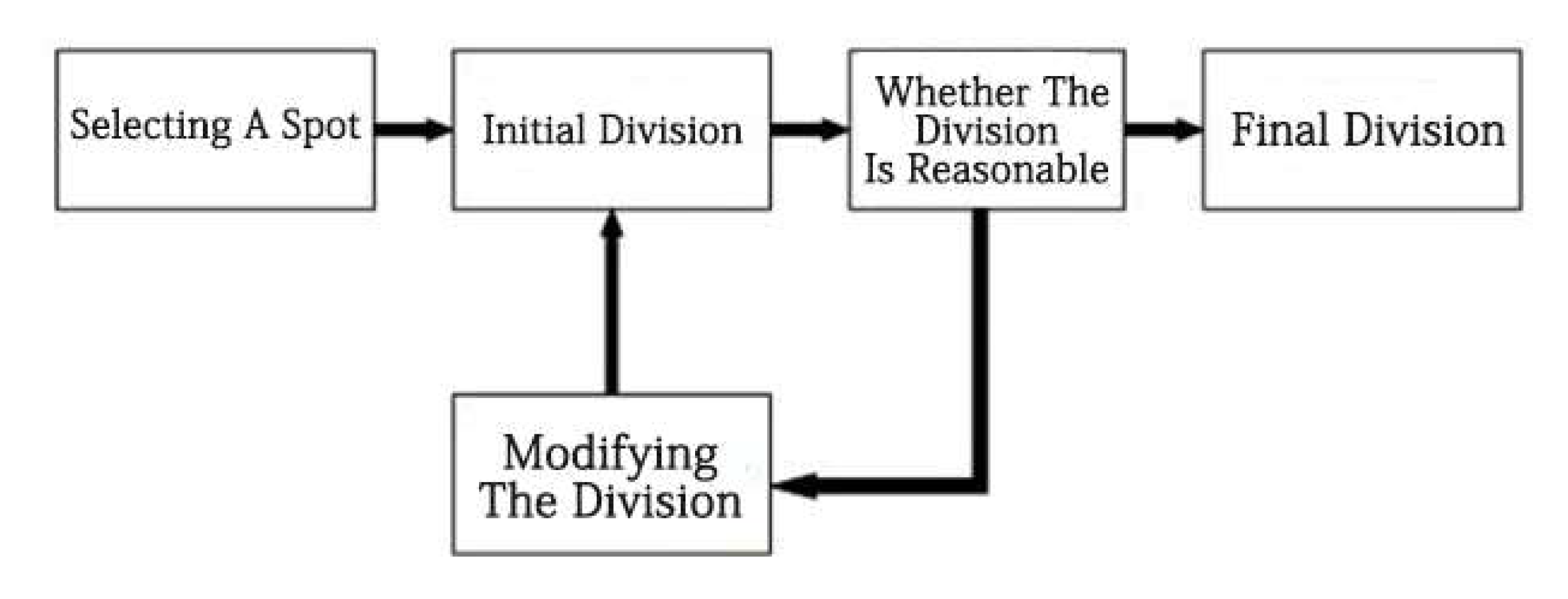
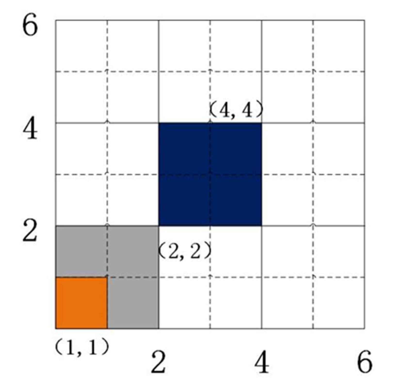
3.1. Adjacent Grid Determination

After the initialization of the grid is completed, the grid is divided into a large granularity grid and small granularity subgrid. Whether the large grid is adjacent to each other is calculated by Equation (2), and the determination of whether the subgrid is adjacent to each other is the same. The process of determining the adjacent grid of the subgrid and large grid is as follows.

(1) Subgrid $w〈V〉=〈V11,V22\dots \dots .Vmm〉$, large grid $W〈V〉=〈V1,V2\dots \dots .Vm〉$

(2) Find the difference between the two vector sets $\Delta \mathrm{V}=\left| \mathrm{w}〈\mathrm{V}〉-\mathrm{W}〈\mathrm{V}〉\right|$

If $\Delta V>2$ exists, the two grids are not adjacent.

If $\Delta V=2$ exists and only one exists and the remaining $\Delta V=0$, then these two grids are adjacent.

If all $\Delta V=1$ or all $\Delta V=2$, then these two lattices are adjacent.

These two lattices are not adjacent in all cases except these three cases.

3.2. Determination of a Boundary Mesh

The density grid-based clustering analysis algorithm is prone to problems such as incorrect data point delineation or missing data points on the boundary grid, leading to a low accuracy of clustering results; therefore, the accurate processing of the boundary grid is of great significance to improve the accuracy of the algorithm. The improved algorithm enhances the processing of the boundary grid compared with the original algorithm, thus improving the quality of the clustering results.

At the beginning of the algorithm, after the grid has been divided, each grid is by default the boundary grid. This is because the internal grid is easier to judge than the boundary grid, and as the whole grid is composed of the internal grid and the boundary grid together, if the grid is not the internal grid, it is the boundary grid. The main steps of the determination algorithm Determination of Boundary () of the boundary grid are shown as Algorithm 1.

Algorithm 1 Steps for determining the boundary grid
Input: Feature vector of the grid to be determined, summary storage mechanism W_List
Output: Bounding mesh identifier Bound
1:	if (adjacent mesh of input mesh does not exist in W_List)
2:	return the grid is a boundary grid
3:	else if (the density of adjacent grid cells of this grid are above the sparsity threshold         Ds or the density of adjacent grid neighboring subgrids is above the subgrid         sparsity threshold Ds_little)
4:	return the grid is an interior grid
5:	else{
6:	return the grid
7:	}//end else if

After determining whether the grid is a boundary grid, the feature vector of the grid is updated, and when the user’s clustering request arrives, the internal grid is processed first and then the boundary grid is processed in the offline stage. The inner grid is usually close to the core of the cluster, while the boundary grid usually consists of a transition or sparse grid.

3.3. Detection and Processing of Isolated Grid Cells

Isolated grid cells are mainly divided into two types: the first type is a grid that has fewer data arriving at the initial stage of the algorithm so that the amount of data is low and cannot reach the specified threshold; the second type is a grid that has more data initially, but fewer data arriving in a period of time, so that the density of the grid cells becomes lower and lower considering the decay factor and eventually fails to reach the threshold. If too much effort is spent on maintaining such grid cells in the algorithm, it will have a significant impact on the efficiency of the whole improvement algorithm, so they should be removed to improve the efficiency of the entire improved algorithm.

Because isolated grid cells are formed by different processes, the methods to remove these two types of isolated grids are also different.

Define the threshold $\rho \left(t_m,t_f\right)$ = $\left({\lambda }^{(-\left(t_m-t_f+T\right)}-1\right)/\left({\lambda }^{(-\left(t_m-t_f\right)}-1\right)$, which is used to avoid the potential for dense grid cells to be removed, where tm represents the current time and t_f represents the time when the data last arrived.

$$\underset{t_{m\to \infty }}{\lim }\rho \left(t_m,t_f\right)=\frac{{\lambda }^{(-(t_m-t_f+T}-1}{{\lambda }^{(-(t_m-t_f}-1}=\frac{\lambda -T-{\lambda }^{\left(t_m-t_f\right)}}{1-{\lambda }^{\left(t_m-t_f\right)}}=\lambda -T$$

(8)

A mesh to be removed that meets this threshold must be a sparse mesh that does not become a potentially dense mesh.

For an isolated grid cell of the first type, if the density of all its subgrid cells is lower than the threshold of subgrid dense grid cells and no data stream arrives in this grid cell in the last interval time T, it is removed, i.e., in addition to satisfying the above threshold, the grid cell satisfies the condition that

$$\left\{\begin{array}{c}\forall D_{little}\left(w,t\right)<{\mathrm{D}}_{t-little}\\ \mathrm{T}\mathrm{w}+\mathrm{T}<\mathrm{t}\end{array}\right.$$

For isolated grid cells of the second type, if all subgrid cells of this grid are below the subgrid density threshold and no data streams have arrived recently, they are not removed during the time period t + T and are not removed if data arrive during the next time period T. Otherwise, the grid cell is removed.

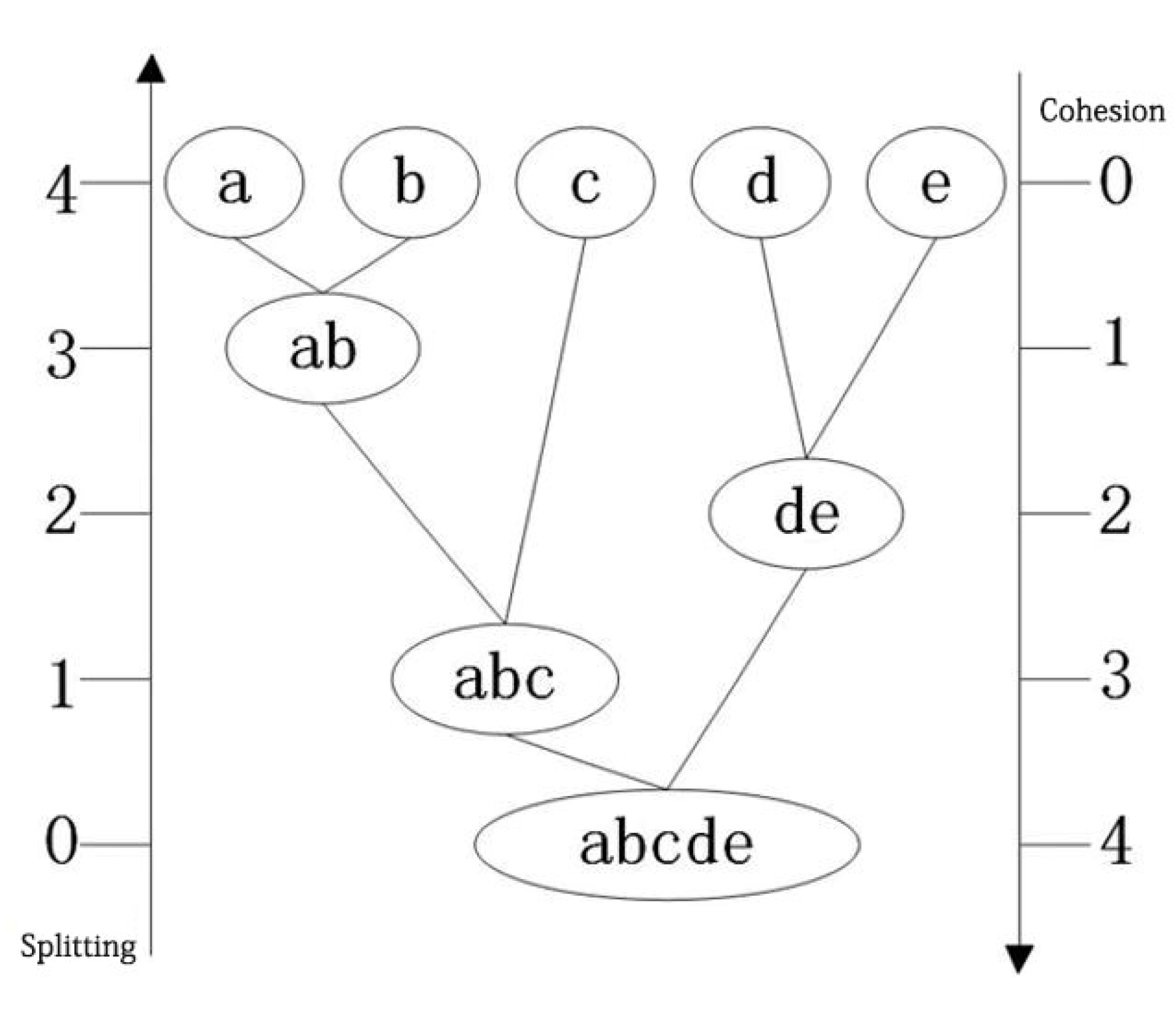
3.4. Microclustering Algorithm

In the process of dynamically receiving real-time data streams, the internal grid is first microclustered using Equation (7) to form initial lattice clusters, which are used as the initial class centers for clustering. When the algorithm runs for a time interval T or a multiple of T, the grid cells are dynamically adjusted. Usually, the larger density grid is regarded as the starting point of clustering, the class attributes in the feature vector are updated, and if an adjacent grid cell of that grid is found, it is grouped into the microclusters as the grid feature vector is updated again, and so on until the search is completed and the first grid cluster is formed. Then, the remaining internal grid cells are processed in the same way, and finally, the set of grid clusters is formed.

The algorithm of microcluster clustering Micro-Cluster() flow is shown in Algorithm 2.

Algorithm 2 Steps of microcluster clustering
Input: the set of internal grid cells in the dynamic grid
Output: set of grid clusters
1:	Detect all internal grid cells and update the grid cell feature vector
2:	While (the class attributes within the set of dynamic internal grid cells no longer change)
3:	{    for(dynamic internal grid cell W1)
4:	{ if(dynamic internal grid cells of W1 exist adjacent to the internal grid W2)
5:	compute Fac(W1,W2);
6:	if (there exists an adjacent grid cell W2 of W1 such that Fac(W1,W2) is maximum)
7:	group grid W2 and W1 into the same cluster.
8:	else group grid W1 as a separate cluster and update flag Cla.
9:	}//end for
10:	}//end while

The final clustering of the offline process uses the grid clusters formed by the microcluster clustering algorithm. This process can be considered as the initial stage of the clustering analysis, and the results of this stage are saved in the grid feature vector.

3.5. Clustering Algorithm for Boundary Subgrids

After obtaining the initial clustering results in the online stage, the main core classes can be obtained. The main purpose of the offline stage is processing the boundary grid, so as to improve the accuracy of the clustering results. The clustering of the boundary grid is based on the existing grid clusters, using fine-grained subgrids for clustering processing. Additionally, using Equation (7), the subgrids are divided and processed for grouping into the nearest and most relevant initial classes, and then the final clustering results are obtained.

The main process of the Boundary sub-grid clustering() algorithm is shown in Algorithm 3.

Algorithm3 Steps of clustering algorithm for boundary subgrid
Input: the boundary grid W1 and its subgrid feature vectors, the set of grid feature vectors
Output: the classes to which the subgrids of grid W1 belong.
1:	obtain information about the boundary grid and its subgrid feature vectors.
2:	if (grid W1 adjacent grid has internal grid)
3:	{ for(internal grid W)
4:	{ for(subgrid cell Wlittle)
5:	{ if(subgrid cell density reaches subgrid density threshold Df-little)
6:	if the subgrid adjacent grid has a large grid that has been divided into     classes, calculate the density factor, group the subgrid into the class where the     grid with the largest Fac is located, and update the subgrid cell feature vector.
7:	else ignore this sub-grid, i.e., the clustering grid density requirement is not met.
8:	}//end for
9:	}//end for
10:	}//end if

The Boundary sub-grid clustering() algorithm divides the subgrid into categories and further processes the boundary grid to improve the quality of the clustering results.

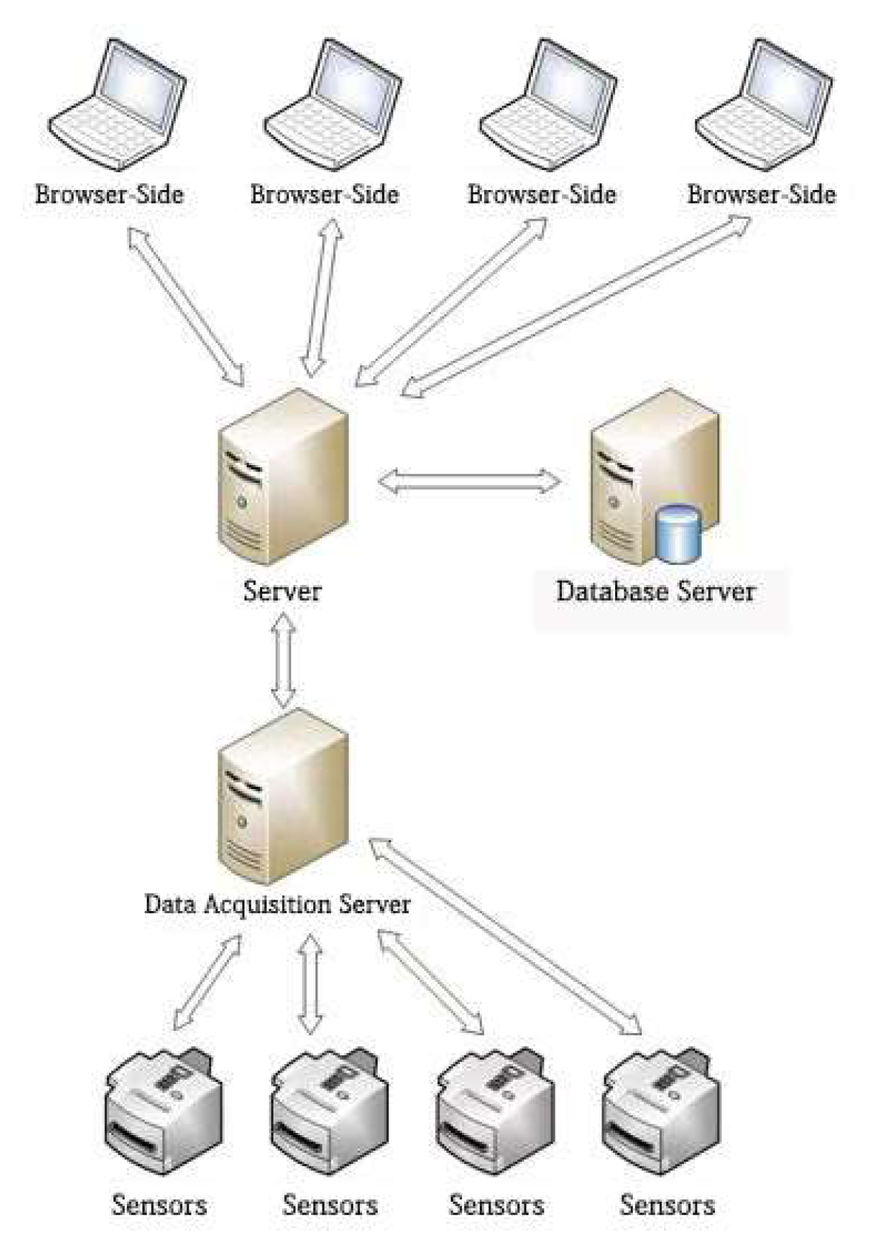
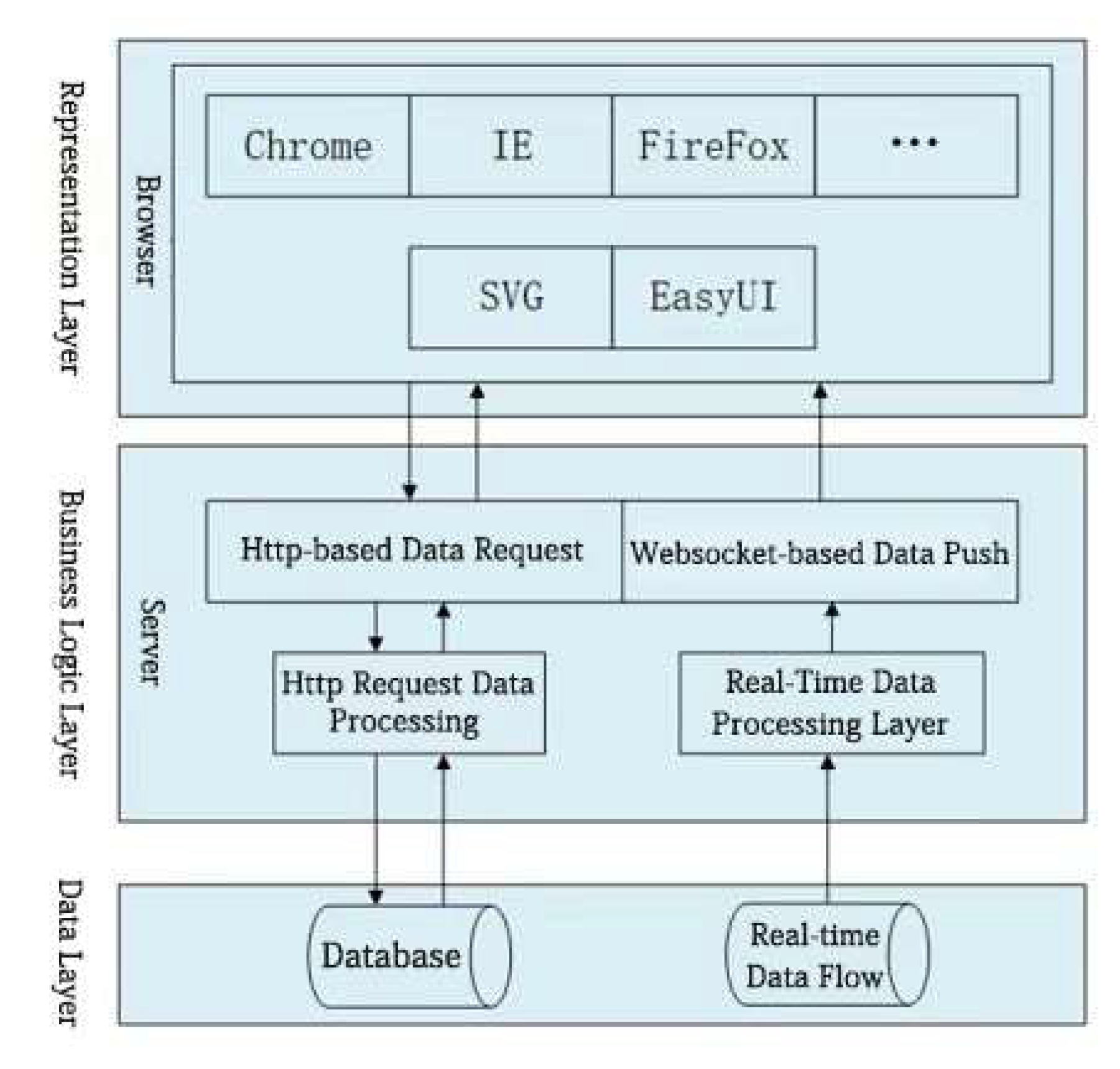
4. Application of the Improved Algorithm in the Corn Storage Monitoring System

The main structure of the corn storage monitoring system is shown in Figure 6. The data streams obtained from the corn quality monitoring sensors are sent to the data acquisition server, which parses the data items and forwards them to the business server. This, in turn, processes them according to the data stream clustering algorithm, thus obtaining the latest status of the corn and displaying it to the user through the browser. This allows the quality status of the corn to be monitored more intuitively.

The main model of the system is shown in Figure 7. The system uses Web-based real-time monitoring. The data flow is processed by the server, the results are delivered to the Web side, and the user can also customize the time for historical queries.

The system is divided into three layers.

(1) Representation layer: this is used to show the monitoring status to the user; it is a dynamic display of the corn quality monitoring status.

(2) Business logic layer: This is used for the business processing of data services and clustering analysis processing of real-time data streams. As the main part of the system, this layer obtains the latest clustering results immediately after pushing them to the front-end page for a real-time response to the monitoring status. In addition, the business logic layer is used to handle other requests from users.

(3) Data layer: this includes the database and the real-time data flow parts of the system, which store the basic information regarding the user and the system and reflects the latest status of the equipment through data collection, respectively.

The improved algorithm is mainly applied in the real-time data flow processing module in the system structure model, which is also the core part of the system. The system acquires real-time data, performs clustering analysis processing, stores and maintains the analysis results in the memory, and sends status information to the front-end page through the clustering result matching analysis.

Together with the corn storage monitoring system module, the steps of the improved algorithm for the real-time data flow processing module are shown in Algorithm 4.

Algorithm4 Steps to improve algorithms in monitoring systems
1:	Initialize the division grid, initialize the grid maintenance cell W_List, current time t;
2:	While (data flow is not finished)
3:	{   read in data item Y, preprocess the data, map to the corresponding grid, update the grid tuple and put it in the data structure information table W_List
4:	if (t = T)//i.e. time reaches the first interval
5:	adjudicate the boundary grid and form the initial grid according to the microcluster clustering algorithm.
6:	if (t > T and t mod T = 0)//that is, the time to reach the second and subsequent intervals
7:	{ decay the grid density according to the decay function and update the grid tuple.
8:	detection and processing of isolated meshes.
9:	adjusting the boundary grid and internal grid information to the density grid microclusters.
10:	starting a new thread to invoke the offline algorithm.
11:	Offline clustering.
12:	Matching analysis results.
13:	Snapshot storage of summary information.
14:	WebSocket message pushing.
15:	}//end if
16:	}//end While

In this system, the improved algorithm processes isolated grids where the data of the isolated grid cells may be anomalous or may be caused by errors during the acquisition process; therefore, its processing differs from the initial algorithm steps. After the isolated grids are acquired, they are analyzed according to user-defined rules, and if there are any abnormalities, they are quickly pushed and saved. Since we are more concerned regarding the monitoring of the most recent time period, this snapshot model stores relevant information for the most recently arrived results with fine granularity.

4.1. Analysis of the Operational Effect of the Improved Algorithm

4.1.1. Operation of the Improved Algorithm

In this study, the data set from a biochemical energy enterprise’s corn storage monitoring system was selected as the test data. The data set included several types of corn moisture content, capacity, and mold grains. Since the original data volume was relatively large, we selected only some of them for testing and used them for comparative analysis experiments.

Table 1. Data from the 20 monitoring sites in the corn storage monitoring data set.

Monitoring Point	Molded Grain %	Moisture Content %	Capacity Weight g/L
1	0.0	10.9	741
2	0.0	11.1	738
3	0.1	11.0	742
4	0.0	12.7	551
5	0.0	12.7	756
6	1.2	12.2	753
7	0.0	12.0	732
8	0.6	15.1	743
9	3.0	12.8	620
10	1.2	17.5	638
11	0.2	13.6	560
12	4.0	10.9	652
13	6.0	10.6	667
14	5.5	10.4	785
15	0.0	9.4	757
16	1.0	22.9	687
17	1.5	21.3	705
18	0.2	22.0	700
19	0.0	12.9	769
20	0.0	13.3	746

shows the data from 20 monitoring points in the maize storage monitoring data set.

The results of the clustering analysis are shown below:

$$\begin{gathered} A=\left[1, 2\left] B=\right[3,5, 6, 15, 20\left] C=\right[4, 11\left] D=\right[7, 19\left] E=\right[8\right] \\ F=\left[9, 10, 12, 13, 16, 17, 18\left] G=\right[14\right] \end{gathered}$$

After clustering the data, the results obtained were matched and analyzed according to the national corn quality indicators (

Table 2. Maize quality indicators.

Grade	Weight Capacity g/L	Mildew Grain Content %	Moisture Content %
1	$\ge$720	$\le$2.0	$\le$14.0
2	$\ge$690
3	$\ge$660
4	$\ge$630
5	$\ge$600
Other	$<$600

) entered by the user, thus enabling real-time monitoring of the quality status of the stored corn. In the data above and in the following table, A, B, and D were first class corn, and C, E, F, and G were unqualified quality corn.

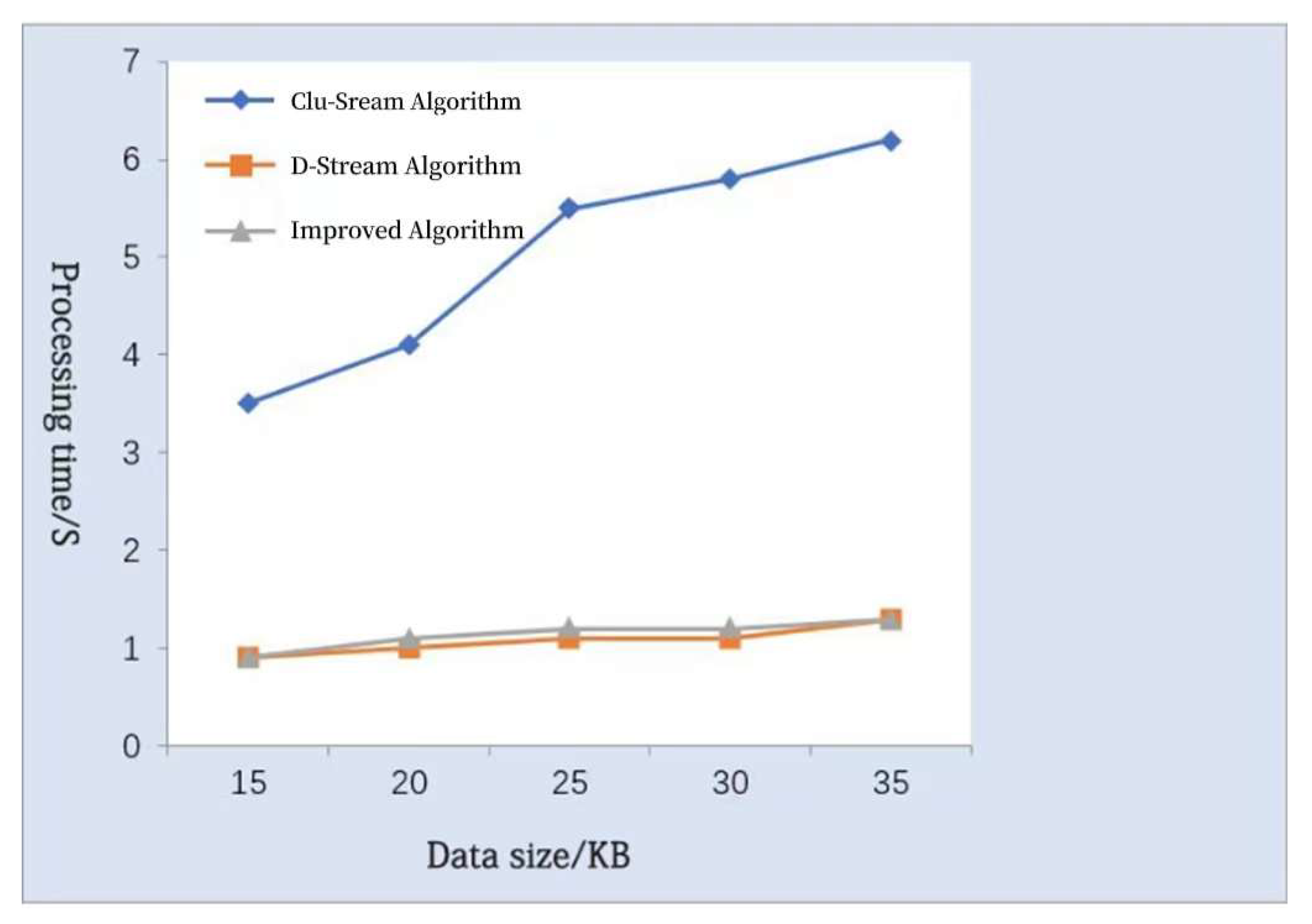
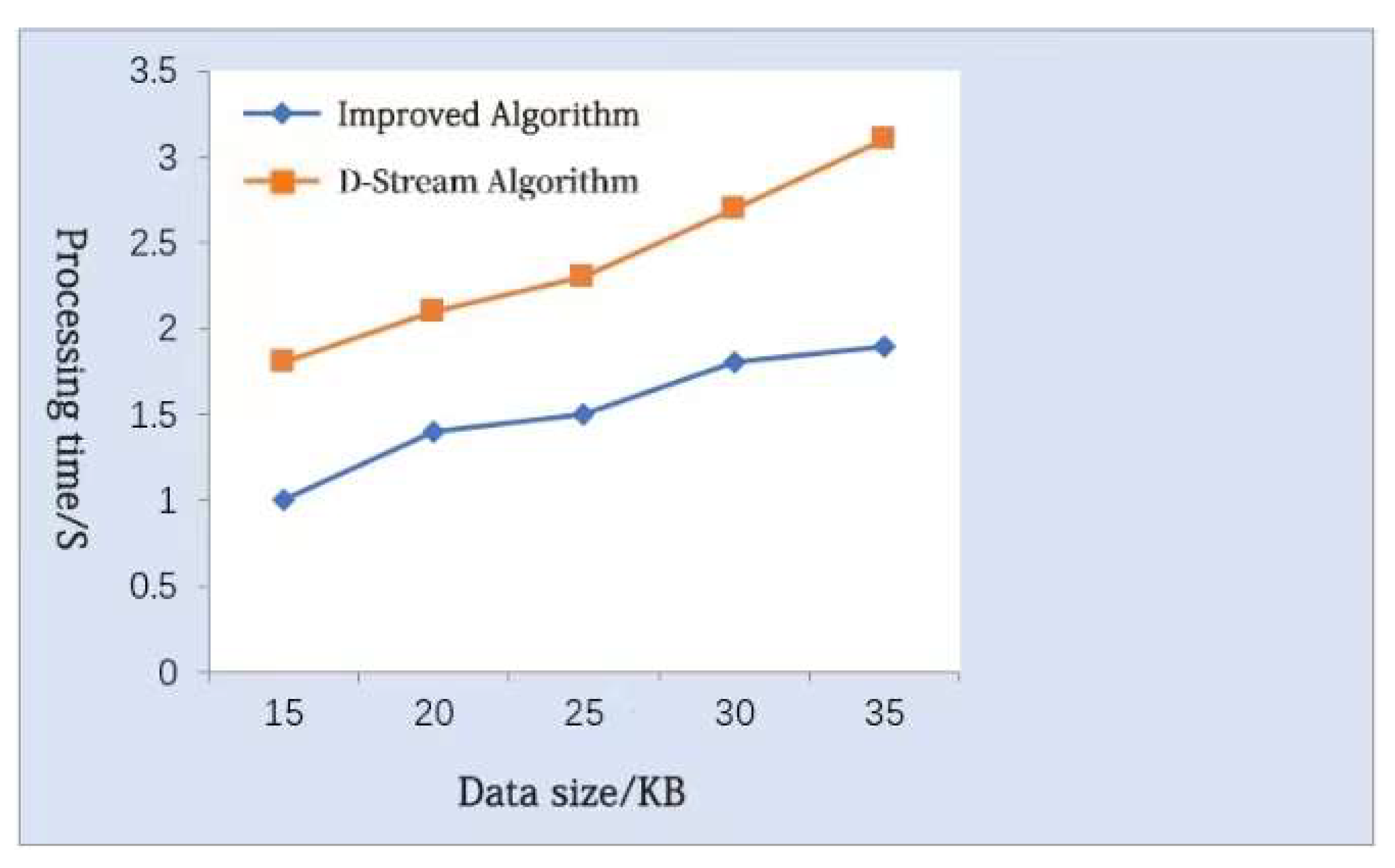
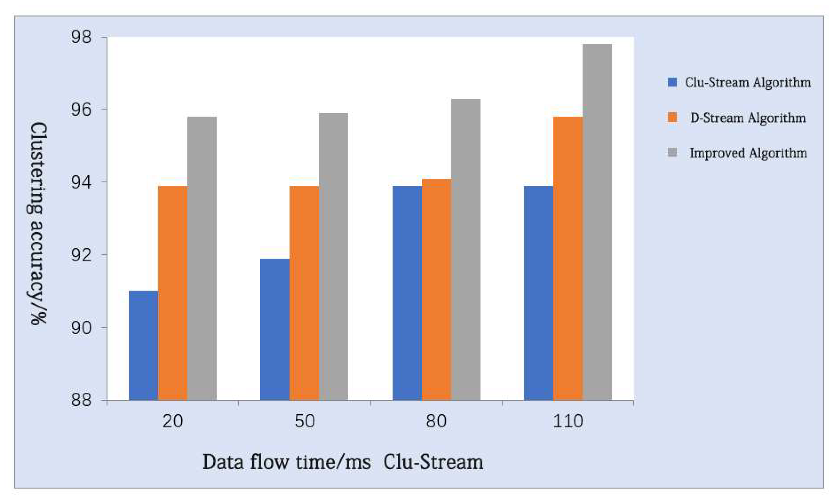
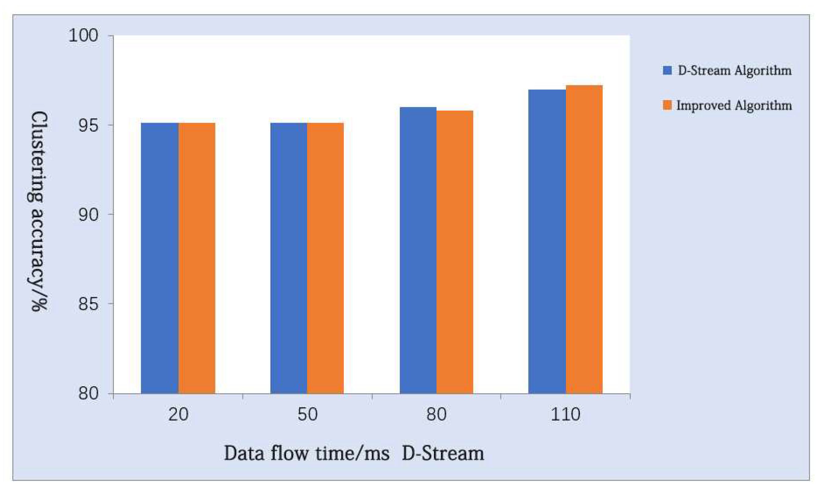
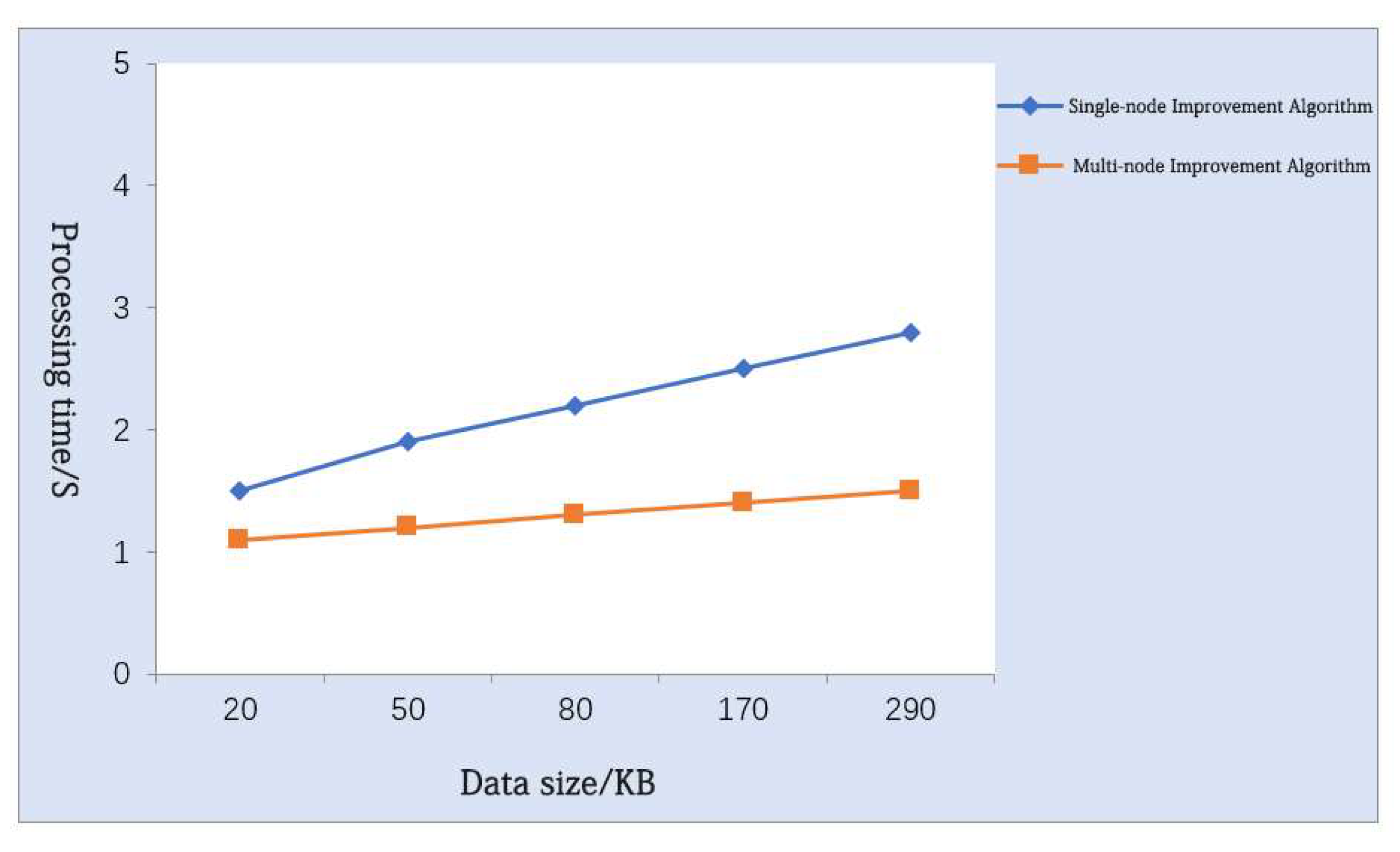
4.1.2. Comparative Analysis of the Improved Algorithms

(1) Comparison and analysis of algorithm running time:

Firstly, we compared the processing time of experimental data ranging from 15 KB to 35 KB under the same running environment, taking the length = 0.065, and comparing the processing time of the Clu-Stream algorithm, the D-Stream algorithm, and the improved algorithm, as shown in Figure 8.

Because both the improved algorithm and the Clu-Stream algorithm directly divide the grid with fine granularity, and the fine granularity of D-stream is equivalent to selecting length/2, the improved algorithm with a grid division of length = 0.065 and the D-Stream algorithm with a grid division of length/2 were selected for comparison. The amount of data selected for the experiments remained in the range of 15 KB to 35 KB, and the processing time results for the comparison are shown in Figure 9.

(2) Comparison of clustering accuracy:

After comparing the clustering runtime, the clustering accuracies of the three algorithms (Clu-Stream, D-Stream, and the improved algorithm) were compared. The clustering accuracy was measured by the intra-group clustering sum (i.e., clustering SSQ), and the clustering accuracy is shown in Figure 10.

Similarly, the improved algorithm with a grid division of length = 0.085 and the D-Stream algorithm with a grid division of length/2 were selected for comparison, with an experimental data volume of 35 KB and different data flow speeds. The results of the comparison clustering accuracy comparison results are shown in Figure 11.

(3) Single-node versus multi-node:

In the previous analysis, we proposed a multi-node processing algorithm in a distributed environment. We used the improved algorithm with a single node and also simulated four local nodes for the comparison experiments below. The amount of experimental data selected was between 20 KB and 290 KB, and the results are shown in Figure 12.

Combining the results of (1) and (2), it can be seen that the processing efficiency of the improved algorithm is greatly superior to that of the Clu-Stream algorithm, in terms of running time under the same experimental environment and experimental data. The more data to be processed, the more obvious the difference between these two algorithms was, but there was almost no difference in the running time when the D-Stream algorithm was used. However, we further compared the processing efficiency of a fine-grained permutation, i.e., D-Stream algorithm at the condition length/2, with that of the improved algorithm, and the results show that the improved algorithm ran almost twice as fast as the D-stream algorithm. In terms of clustering accuracy, the improved algorithm was more accurate than the Clu-Stream algorithm and the D-Stream algorithm and was comparable with the D-Stream algorithm under the fine-grained partitioning condition. Additionally, we observed that the slower the data stream arrived, the better the algorithm clustered. In summary, we can conclude that the improved algorithm improves the clustering accuracy on the basis of guaranteed running time.

From the results of (3), we can observe that the multi-node approach in a distributed environment improves the running time of the improved algorithm, and the advantage of this approach compared with a single node is more obvious when the amount of data is larger, meaning that it can be used when the data stream is processed too fast.

5. Conclusions

Today, green, ecological, and sustainable energy-saving storage technology is the direction of travel for the scientific and technological development of grain storage. The data flow monitored by corn storage systems is high-speed, continuous, and real-time, whereas the traditional cluster analysis algorithm is primarily intended for static data information processing. In this study, we addressed the shortcomings of the algorithm and proposed an improved algorithm for the clustering analysis of real-time data streams based on density grid; on its insufficient processing of boundary grid and single-node uniform division of the grid problem. The algorithm is based on a two-stage processing framework of online and offline processing. The algorithm adopts a grid partitioning strategy with different granularities of coarse and fine, clustering the internal grid with a coarse-grained grid based on the grid influence factor, and processing the boundary grid with fine-grained clustering. It also includes dynamic adjustment of the grid density threshold, and detection and processing of isolated grids, which improves its efficiency. The dynamic density threshold is used in the improved algorithm, and the incremental algorithm calculates the center of mass, which better reflects the real-time change in the data and the processing of isolated grids, improving the efficiency of the algorithm. We also propose a local and global node processing model for this algorithm in a distributed environment, which once again improves its processing speed.

The algorithm was run in a green storage monitoring system for corn, and the clustering accuracy and the processing efficiency were verified by comparison tests with the Clu-stream and D-stream algorithms. Finally, the algorithm was applied to the green storage monitoring system for corn belonging to a biochemical energy enterprise. Through experimental comparison and analysis, it was shown that the improved algorithm had a higher clustering accuracy, a stable and real-time running state, and good performance. It can successfully ensure that corn is stored in a green way that is green, safe, and efficient, thus contributing to the achievement of sustainability goals.

From our results, one potential future research direction is to compare our im-proved optimization algorithms with other proposed ones in the literature, or new al-gorithms can be designed and compared with the ones applied to this study. To im-prove the accuracy of our clustering while ensuring less predictable errors, the logistics regressions can be combined with our algorithms. More analyses for the calibration and tuning of our methods can be done to improve the efficiency of our optimization algorithm. Finally, different real-time optimization policies and strategies can be ex-tracted from the literature to further analyze our results as an extension of this paper.

References

1. Rostamzadeh, R.; Govindan, K.; Esmaeili, A.; Sabaghi, M. Application of fuzzy VIKOR for evaluation of green supply chain management practices. Ecol. Indic. 2015, 49, 188–203. [Google Scholar] [CrossRef]
2. Kumar, N.; Agrahari, R.P.; Roy, D. Review of green supply chain processes. Ifac-Pap. 2015, 48, 374–381. [Google Scholar] [CrossRef]
3. Mao, J.; Sun, Q.; Ma, C.; Tang, M. Site selection of straw collection and storage facilities considering carbon emission reduction. Environ. Sci Pollut Res. 2021. [Google Scholar] [CrossRef]
4. Mao, J.; Hong, D.; Chen, Z.; Changhai, M.; Weiwen, L.; Wang, J. Disassembly sequence planning of waste auto parts. J. Air Waste Manag. Assoc. 2021, 71, 607–619. [Google Scholar] [CrossRef] [PubMed]
5. Jiang, X.; Tian, Z.; Liu, W.; Tian, G.; Gao, Y.; Xing, F.; Suo, Y.; Song, B. An energy-efficient method of laser remanufacturing process. Sustain. Energy Technol. Assess. 2022, 52, 102201. [Google Scholar] [CrossRef]
6. Yin, Y.X.; Chen, L.; Meng, Z.; Li, B.; Luo, C.; Fu, W.; Mei, H.; Qin, W. Design and evaluation of a maize monitoring system for precision planting. Int. J. Agric. Biol. Eng. 2018, 11, 166–170. [Google Scholar] [CrossRef]
7. Irmak, S.; Haman, D.Z.; Bastug, R. Determination of Crop Water Stress Index for Irrigation Timing and Yield Estimation of Corn. Agron. J. 2000, 92, 1221–1227. [Google Scholar] [CrossRef]
8. Holmes, M.; Renk, J.S.; Coaldrake, P.; Kalambur, S.; Schmitz, C.; Anderson, N.; Gusmini, G.; Annor, G.; Hirsch, C.N. Food-Grade Maize Composition, Evaluation, and Genetics for Masa-Based Products. Crop Sci. 2019. [Google Scholar] [CrossRef]
9. Pippenger, N.; Segall, R.S.; Berleant, D.; Eversole, K.A.; Mustell, R.A.; Hood, E.E. Extracting Numerical Information about Corn Composition from Texts (Invited Paper). J. Syst. Cybern. Inform. 2015, 13, 68–75. [Google Scholar]
10. Ni, B.; Paulsen, M.R.; Reid, J.F. Corn Kernel Crown Shape Ientification Using Image Processing. Trans. ASAE 1997, 40, 833–838. [Google Scholar] [CrossRef]
11. Wang, W.C.; Wang, L. Design of Moisture Content Detection System. Phys. Procedia 2012, 33, 1408–1411. [Google Scholar] [CrossRef] [Green Version]
12. Tan, L.B.; Ji, H.Y. Study on Grain Moisture Detection System Based on the Theory of Dielectric Properties. Appl. Mech. Mater. 2013, 333–335, 1558–1563. [Google Scholar] [CrossRef]
13. Zhao, X.; Wei, J.; He, L.; Zhang, Y.; Zhao, Y.; Xu, X.; Wei, Y.; Ge, S.; Ding, D.; Liu, M.; et al. Identification of Fatty Acid Desaturases in Maize and Their Differential Responses to Low and High Temperature. Genes 2019, 10, 445. [Google Scholar] [CrossRef] [PubMed]
14. Sanjeev, P.; Chaudhary, D.P.; Sreevastava, P.; Saha, S.; Rajenderan, A.; Sekhar, J.C.; Chikkappa, G.K. Comparison of Fatty Acid Profile of Specialty Maize to Normal Maize. JAOCS. J. Am. Oil Chem. Soc. 2014, 91, 1001–1005. [Google Scholar] [CrossRef]
15. Lam, H.S.; Proctor, A. Rapid Methods for Milled Rice Surface Total Lipid and Free Fatty Acid Determination. Cereal Chem. 2001, 78, 498–499. [Google Scholar] [CrossRef]
16. Dou, Y.P. Determination of fatty acid values of corn by potentiometric titration. Grain Oil Storage Sci. Technol. Commun. 2004, 3, 47–49. [Google Scholar]
17. Liu, Y.; Zhai, H.B.; Cai, J.P. Early warning of aflatoxin production in stored maize using monitoring CO2 method. Mod. Food Sci. Technol. 2015, 31, 309–315. [Google Scholar]
18. Huichun, Y.U.; Lou, N.; Yin, Y.; Liu, Y. Study on Detection Model of Maize Toxin with Algorithm of SPXY and SPA Based on Hyperspectral Technology. Food Sci. 2018, 39, 328–335. [Google Scholar]
19. Techniques for the Discovery of Patterns Hidden in Large Data Sets and Process Flow of Data Mining. Int. J. Innov. Technol. Explor. Eng. 2019, 9, 2480–2483. [CrossRef]
20. Tencent Technology (Shenzhen, China) Company Limited. Data Batch Processing Method and System. US Patent 10,803,433, 13 October 2020.
21. Victorovich, K.K. A Multilevel Scheduling Model for Data Batches Processing in Conveyor Systems when Forming Sets and in the Presence of Restriction. SPIIRAS Proc. 2016, 4, 65. [Google Scholar] [CrossRef]
22. Goudarzi, M. Heterogeneous Architectures for Big Data Batch Processing in MapReduce Paradigm. IEEE Trans. Big Data 2019, 5, 18–33. [Google Scholar] [CrossRef]
23. Hensel, C.; Junges, S.; Katoen, J.; Quatmann, T.; Volk, M. The probabilistic model checker Storm. Int. J. Softw. Tools Technol. Transf. 2022, 24, 589–610. [Google Scholar] [CrossRef]
24. Research on Real-Time Anomaly Detection of Massive Log Streams Based on DME Cluster Analysis Model; Hangzhou University of Electronic Science and Technology: Hangzhou, China, 2017.
25. Chen, F.M.; Han, D.Z.; Bi, K.; Dai, Y.T. Exploration of key technologies for distributed data stream processing in big data environment. Comput. Appl. 2017, 37, 620–627. [Google Scholar] [CrossRef]
26. Chen, F. Research and Application of Data Stream Anomaly Detection Technology. Available online: https://kns.cnki.net/kcms/detail/detail.aspx?dbcode=CMFD&dbname=CMFD2011&filename=2010234254.nh&uniplatform=NZKPT&v=SwOVri0cKXGi4psyVacEyw4DekFbZXLvDIkK2-b8EvXAWNNBPcQa8ronLw8XZ7fD (accessed on 22 July 2022).
27. Knorr, E.M.; Ng, R.T.; Tucakov, V. Distance-based outliers: Algorithms and applications. VLDB J. 2000, 8, 237–253. [Google Scholar] [CrossRef]
28. Knorr, E.M.; Ng, R.T. Algorithms for Mining Distance-Based Outliers in Large Datasets. In Proceedings of the International Conference on Very Large Data Bases, New York, NY, USA, 24–27 August 1998; pp. 392–403. [Google Scholar]
29. Kumar, P.K.; Diwakar, S. Maxmin distance sort heuristic-based initial centroid method of partitional clustering for big data mining. Pattern Anal. Appl. 2022, 25, 139–156. [Google Scholar] [CrossRef]
30. Kamlesh, P.K.; Diwakar, S. Maxmin Data Range Heuristic-Based Initial Centroid Method of Partitional Clustering for Big Data Mining. Int. J. Inf. Retr. Res. (IJIRR) 2021, 12, 1–22. [Google Scholar] [CrossRef]
31. Narjes, V.; Mirzabeigi, M.; Sotudeh, H.; Fakhrahmad, S.M. Application of k-means clustering algorithm to improve effectiveness of the results recommended by journal recommender system. Scientometrics 2022, 127, 3237–3252. [Google Scholar] [CrossRef]
32. Awad, F.H.; Hamad, M.M. Improved k-Means Clustering Algorithm for Big Data Based on Distributed SmartphoneNeural Engine Processor. Electronics 2022, 11, 883. [Google Scholar] [CrossRef]
33. Bock, F. Hierarchy cost of hierarchical clusterings. J. Comb. Optim. 2022, 44, 617–634. [Google Scholar] [CrossRef]
34. Naik, C.; Shetty, P.D. FLAG: Fuzzy logic augmented game theoretic hybrid hierarchical clustering algorithm for wireless sensor networks. Telecommun. Syst. 2022, 79, 559–571. [Google Scholar] [CrossRef]
35. Khader, M.; Al-Naymat, G. An overview of various enhancements of DENCLUE algorithm. In Proceedings of the DATA’19: International Conference on Data Science, E-learning and Information Systems 2019, Dubai, United Arab Emirates, 2–5 December 2019. [Google Scholar] [CrossRef]
36. Alexander, K.; Peciar, P.; Coffey, K.; Bryan, K.; Lenihan, S. A combination of density-based clustering method and DEM to numerically investigate the breakage of bonded pharmaceutical granules in the ball milling process. Particuology 2021, 58, 153–168. [Google Scholar] [CrossRef]
37. Kazemi, U.; Boostani, R. FEM-DBSCAN: An Efficient Density-Based Clustering Approach. Iran. J. Sci. Technol. Trans. Electr. Eng. 2021, 45, 979–992. [Google Scholar] [CrossRef]
38. Suo, M.L.; Zhou, D.; Ruoming, A.; Shunli, L. Neighborhood density grid clustering algorithm and application. J. Tsinghua Univ. 2018, 58, 732–739. [Google Scholar] [CrossRef]
39. Weber, C.M.; Ray, D.; Valverde, A.A.; Clark, J.A.; Sharma, K.S. Gaussian mixture model clustering algorithms for the analysis of high-precision mass measurements. Nucl. Inst. Methods Phys. Res. 2022, 1027, 166299. [Google Scholar] [CrossRef]
40. García-Escudero, L.A.; Mayo-Iscar, A.; Riani, M. Constrained parsimonious model-based clustering. Stat. Comput. 2021, 32, 2. [Google Scholar] [CrossRef] [PubMed]
41. Mohammadi, M.; Gheibi, M.; Fathollahi-Fard, A.M.; Eftekhari, M.; Tian, G. A hybrid computational intelligence approach for bioremediation of amoxicillin based on fungus activities from soil resources and aflatoxin b1 controls. J. Environ. Manag. 2021, 299, 113594. [Google Scholar] [CrossRef]
Figure 1. Block diagram of the delineation clustering algorithm.
Sustainability 14 10822 g001
Figure 2. Coalescent and split-level clustering on the set of data objects {a, b, c, d, e}.
Sustainability 14 10822 g002
Figure 3. Grid division.
Sustainability 14 10822 g003
Figure 4. The 4-connection.
Sustainability 14 10822 g004
Figure 5. The 8-connection.
Sustainability 14 10822 g005
Figure 6. System structure diagram.
Sustainability 14 10822 g006
Figure 7. System architecture model diagram.
Sustainability 14 10822 g007
Figure 8. Comparison of processing time of Clu-Stream algorithm, D-Stream algorithm, and improved algorithm.
Sustainability 14 10822 g008
Figure 9. Comparison of processing time of D-Stream algorithm (length/2) and improved algorithm (length).
Sustainability 14 10822 g009
Figure 10. Comparison of clustering accuracy of Clu-Stream algorithm, D-Stream algorithm, and improved algorithm.
Sustainability 14 10822 g010
Figure 11. Comparison of clustering accuracy of D-Stream algorithm and improved algorithm.
Sustainability 14 10822 g011
Figure 12. Comparison of the running time of the improved algorithm under single-node and multi-node conditions.
Sustainability 14 10822 g012