Prediction of Ground Water Content Using Hyperspectral Information through Laboratory Test

Abstract

With the technological advances led by the fourth industrial revolution, automation has been implemented in road earthworks and paving in the road construction sector. For preparation of construction works, achieving an optimal degree of compaction of the subgrade soil is one of the key factors required for automation of construction and digitalization of quality control. The degree of compaction is greatly affected by water content in geotechnical aspects, and measurement of water content is a necessary process in construction sites. However, conventional methods of water content measurement have limitations and drawbacks and have low efficiency considering the recent trend of construction automation and digitalization of quality control. Therefore, in this study, hyperspectral remote sensing was applied for efficient large-scale measurement of water content over a wide area. To this end, first, through laboratory tests, soil water content was normalized with spectral information. A spectrum was derived with a varying water content using standard sand, and reflectance was obtained for specific ranges of wavelength. Finally, we obtained the relationship between the reflectance and the water content by comparing with various fitting models. At this time, the ranges of wavelength to be used in the equation were specified and presented in an exponential model.

1. Introduction

One of the main goals of the 4th industrial revolution is to accomplish groundbreaking innovation in industrial productivity through convergence of various information and communication technologies (ICT) and digital technologies such as artificial intelligence, the Internet of Things, and big data. The implementation of intelligent information technologies and the impact of technological advancement resulted in transformational changes in economic and social dimensions [1]. However, the construction industry has experienced relatively few changes during the fourth industrial revolution because of the conservative or traditional nature of the industry, compared to other sectors. This led to a number of challenges in the construction industry, and in recent trends for active implementation of the fourth industrial revolution, digitalization and introduction of innovative technologies has occurred in the industry [2]. Among the various fields of the construction industry, the road construction sector has shown some progress in research on digitalization and automation for productivity enhancement and improvement in quality control. Representative examples include utilization of unmanned aerial vehicles (UAVs), 3D laser scanning, building information modeling (BIM), and automated (unmanned) construction using robots, as well as improved construction materials [3].

Road earthworks and paving form the basis of the road construction sector, and it has been reported that, as these works are carried out linearly with repetitive processes, the application of automated construction is relatively straightforward [4,5]. However, this is true only for the introduction of automation equipment related to construction. In contrast, in the case of obtaining the required degree of compaction of the subgrade soil, which is performed prior to construction, the work entails considerable variability depending on the ground conditions. This variability in the work has a significant impact on the construction automation and digitization of quality control.

An optimal degree of subgrade compaction ensures road performance and quality, whereas substandard compaction significantly compromises the modulus and integrity of the subgrade [6]. The degree of compaction is represented as the ratio of the dry unit weight in the construction site to the maximum unit weight and is directly related to the water content in the ground. According to the standard compaction test [7], when the same compaction energy is applied to the ground, the compaction curve for the dry unit weight of the soil has an inverted parabolic shape as a function of water content. Its maximum value corresponds to the optimum water content. That is, the degree of compaction cannot reach 100% if the water content is not optimum, and energy greater than the standard energy needs to be applied. The variation in soil water content has a significant impact on the bearing capacity, soil deformation characteristics, and as a result, stability of earth structures [8]. That is, the interplay between water content and degree of compaction plays a key role in terms of long-term stability and long-term serviceability of engineered earth structures [9]. Therefore, determination of soil water content is an essential prerequisite to achieve accurately designed compaction.

In general, for in situ determination of soil water content at construction sites, conventional methods (measurement of water content by gravimetric analysis of the weight of an in situ soil sample and the weight of the dried sample) are applied. These methods tend to be time-consuming, unreliable owing to the difference in error range, depending on the proficiency of individual operator, and provide information point-by-point rather than over an area. Thus, conventional methods are limited in reflecting the overall conditions of construction sites. In order to resolve these problems, time-domain reflectometry (TDR) and ground-penetrating radar (GPR) have been employed to determine soil water content [10,11,12,13,14,15]. TDR uses an instrument that measures the time it takes for a pulse signal to return, and GPR performs measurements of volumetric water content and dielectric constant. However, these methods also have limitations in terms of implementing automation, because they cannot measure water content of the entire construction site, are time-consuming or require manual inputs in the process of data measurement.

In this study, we address the limitations of the conventional methods of water content measurement by introducing hyperspectral remote sensing, wherein water content is measured over a wide area and data are constructed based on the measurements. Hyperspectral remote sensing facilitates the construction automation and digitalization of quality control. In the construction industry, hyperspectral remote sensing has mainly been employed for classification of mineral types, particle sizes, and qualities or for the development of new vegetation parameters or vegetation indices [16,17,18,19]. In terms of water-related measurements, the technology has been applied to measurements of water quality parameters or water content in plants [20,21,22]. Research on soil water content has been less conducted to date, and whenever the technology of hyperspectral remote sensing can be applied, large-scale water content measurements can be carried out over a wide area.

Hyperspectral images may be used through spectral image fusion using different sensors or different spectral ranges, depending on the purposes of applications. Hyperspectral images have a complex data structure due to the presence of more bands than in conventional spectral images. For visual observation of hyperspectral images, the image for each band is visualized individually. Alternatively, in the case of hyperspectral images in the VNIR range, VNIR hyperspectral images are reconstructed into Rend-Green-Blue (RGB) images for visualization, based on the intensity of the RGB bands [23]. The basic spectrum of remote sensing is a function of wavelength and is expressed in terms of apparent spectra of reflectance distribution. Spectral reflectance is used to determine properties of the chemical and physical composition of individual matter, including molecular and electronic resonances, as well as surface and bulk structures [24].

The final objective of this study is to mount a hyperspectral camera on a drone, a UAV, and to convert the hyperspectral information captured over a wide area by the camera into water content. With the aim of this study as described above, laboratory tests were performed to carry out normalization of water content using spectral information. To this end, ground specimens containing different water contents were obtained, and a system for the acquisition of hyperspectral information of the ground was constructed. For the soil used in the experiment, well-known standard sand was used considering normalization, and the water content composition varied from 0 to 21% in 1% increments. The hyperspectral information acquired through the constructed system was reflectance by the wavelength range, and 1:1 matching with water content was not possible. Consequently, the hyperspectral information was converted into spectrum indices proposed in previous studies [25,26,27]. In this case, when the reliability of the water content prediction by existing methods was questionable, a new equation for the estimation of the spectrum index was applied.

2. Methodology

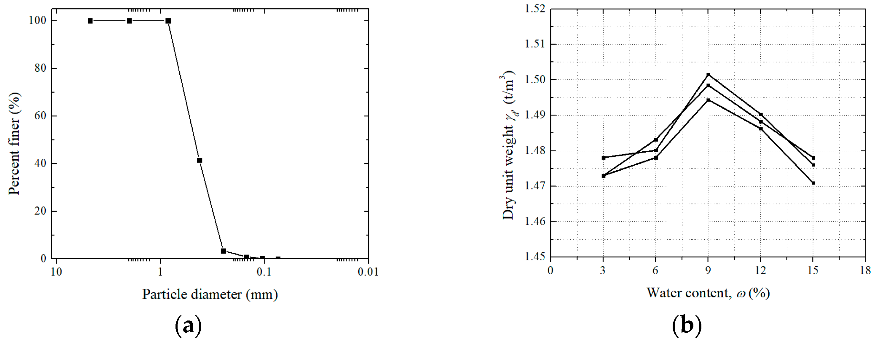
2.1. Material Properties of Soil

Standard sand that allowed for the acquisition of ideal experimental results, normalization of data, and ensured reliability was selected as the soil for the experiment. For the analysis of the material properties of the selected soil, the sieve test according to ASTM D422 [28] and the standard compaction test of ASTM D698 [7] were performed. The results are presented in Figure 1 and

Table 1. Sieve analysis results of the used sand.

D10 1 (mm)	D30 2 (mm)	D60 3 (mm)	Coefficient of Uniformity, Cu	Coefficient of Curvature, Cc	Percent Passing No. 200 Sieve (%)	Soil Classification Based on USCS [30]
0.270	0.358	0.527	1.952	0.901	0.06	SP

¹ D₁₀: particle diameter in percent finer of the soil corresponding to 10%; ² D₃₀: particle diameter in percent finer of the soil corresponding to 30%; ³ D₆₀: particle diameter in percent finer of the soil corresponding to 60%.

.

Figure 1a and Table 1 represent the sieve test results. The particle size range of the selected soil met the range specified in ISO 679 (0.08–2.00 mm) [29], which is the range of standard sand. In Table 1, D₁₀, D₃₀, and D₆₀ are the particle sizes at which 10%, 30%, and 60% of the soil particles are finer, respectively. Furthermore, the coefficient of uniformity (C_u = D₆₀/D₁₀) and the coefficient of curvature (C_c = D₃₀²/(D₁₀D₆₀)) are presented. Based on the test results, the soil used in the experiment was classified as poorly graded sand (SP) according to the Unified Soil Classification System (USCS) of ASTM D2487 [30]. Figure 1b shows the result of the compaction test. The maximum unit weight (γ_d,max) of the sand was 1.498 t/m³, and the optimum water content (ω_opt) was 9%.

2.2. Laboratory Test to Obtain Hyperspectral Information

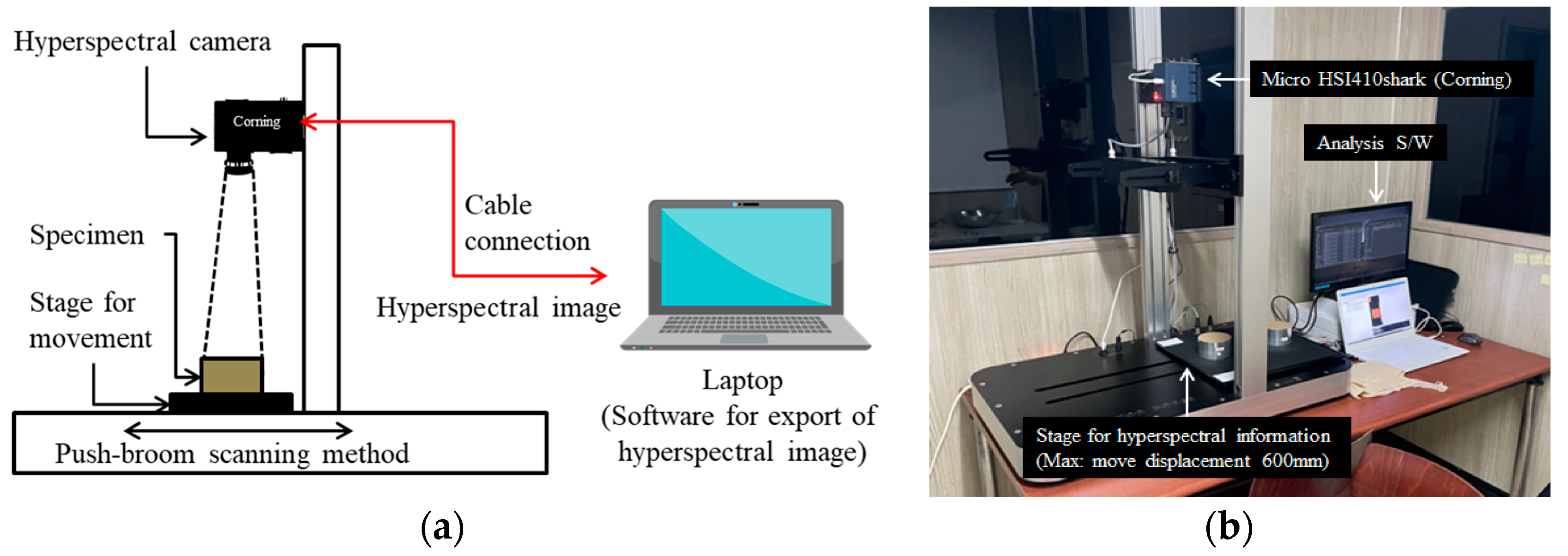
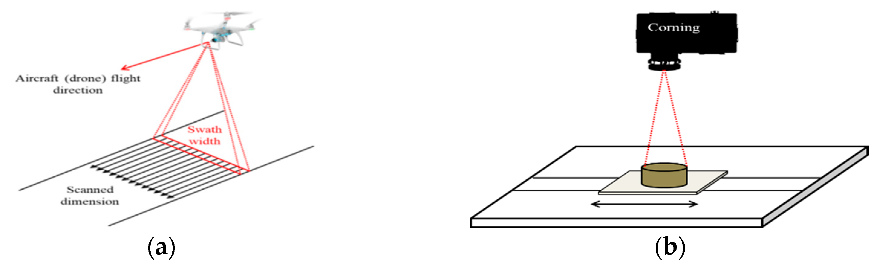
2.2.1. Analysis System to Obtain the Hyperspectral Information of the Soil

For the acquisition of hyperspectral information according to the water content condition of the sand, a laboratory test system was set up, as shown in Figure 2. The system consisted of a hyperspectral camera, a stage for mounting and moving the specimen, and a laptop for running software.

The hyperspectral camera (Micro HSI410shark, Coring, NY, USA) was a VNIR camera capable of measuring wavelengths from 380 to 1000 nm with a spectral resolution of 2 nm. In the setup, the hyperspectral camera was installed at a suitable height considering the field of view and focus. A specimen was mounted on a stage, moved according to the push-broom scanner method and was captured from a hyperspectral camera above. For all experimental processes, including command and control, in-house software pre-programmed in an embedded processor (a laptop in this study) was used.

In general, the main scanning approaches used for a spectral camera include staring or spectral scanning, which captures the entire scene in the band-sequential format, and push-broom scanning, which generates hyperspectral images according to the line-by-line scanning method [31]. In staring or spectral-scanning, the number of spectrum filters is small and the resolution is limited, whereas push-broom scanning allows for a reasonable range of spatial resolution and high spectral resolution [32].

Therefore, in this study, push-broom scanning was adopted as a method of capturing images with the hyperspectral camera for water content measurement. This method has been applied in previous studies, and its reliability can be considered to be verified through the results reported therein [33,34,35,36,37].

Furthermore, push-broom scanning was selected in this study, because the technology was applied to a UAV later on. Push-broom scanning is the most common method of acquiring spectral images through flight vehicles such as UAVs or airborne systems. As shown in Figure 3a, a hyperspectral camera (or sensor) is mounted on an aircraft (drone) with a slit perpendicular to the forward flight direction of the drone. In a typical spectral camera, the spectrum is measured according to the width of the pixel (equal to the scanning range on the ground), which is determined by the detection interval, focal length, and flight altitude. The camera mounted on the drone measures the spatial spectrum frame of a specific pixel and measures the frame of the line corresponding to the next pixel while moving. In this way, the designed system is able to capture the 2D image width [24].

In this way, push-broom scanning is applied to the analysis system herein, and the moving part is installed on the stage where the specimen is set, rather than by means of the aircraft moving, as shown in Figure 3b. Therefore, the hyperspectral camera was fixed in the experimental setup of this study, and the spectral information of the soil in the specimen was scanned according to the movement of the moving part of the stage.

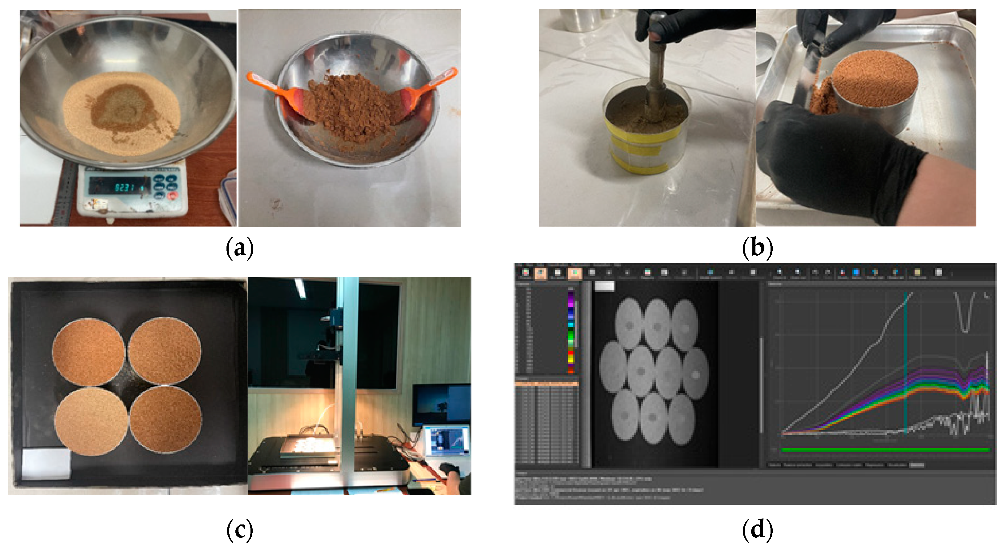
2.2.2. Procedure to Obtain Hyperspectral Information about Water Content

In this study, for the acquisition of hyperspectral information under different water content conditions, specimens were prepared as shown in Figure 4. The experimental conditions were as follows. The range of the water content condition was 0–21%, with an increment in the water content of 1%, and the degree of compaction of the specimens was set to 95%, being the optimal degree of compaction of the subgrade soil.

Here, the water content was the weight ratio of soil and water, and water as much as the water content corresponding to the weight of the sample soil was added and mixed. The volume of the used cylinder can (diameter = 10 cm; height = 6 cm) was 471 cm³, and the cylinder contained up to 705 g of soil according to the compaction result in Figure 4a. In this study, a degree of compaction of 95% was aimed at, and about 670 g of sand were used for each test. At this time, the water content was 0–21% for 670 g of soil as shown in Figure 4a. For example, in the condition of 1% water content, 6.7 g of water were added and mixed. When mixing was complete, compaction was performed, so that all of the soil mixed according to the water content was included inside the circular can, as shown in Figure 4b. At this time, the test was conducted very elaborately. As a result of re-measurement of the water content after all the experimental procedures, it was confirmed that the water content was the same as immediately after production. This means that the test case accurately reflected the water content in the spectral information acquisition experiment performed later.

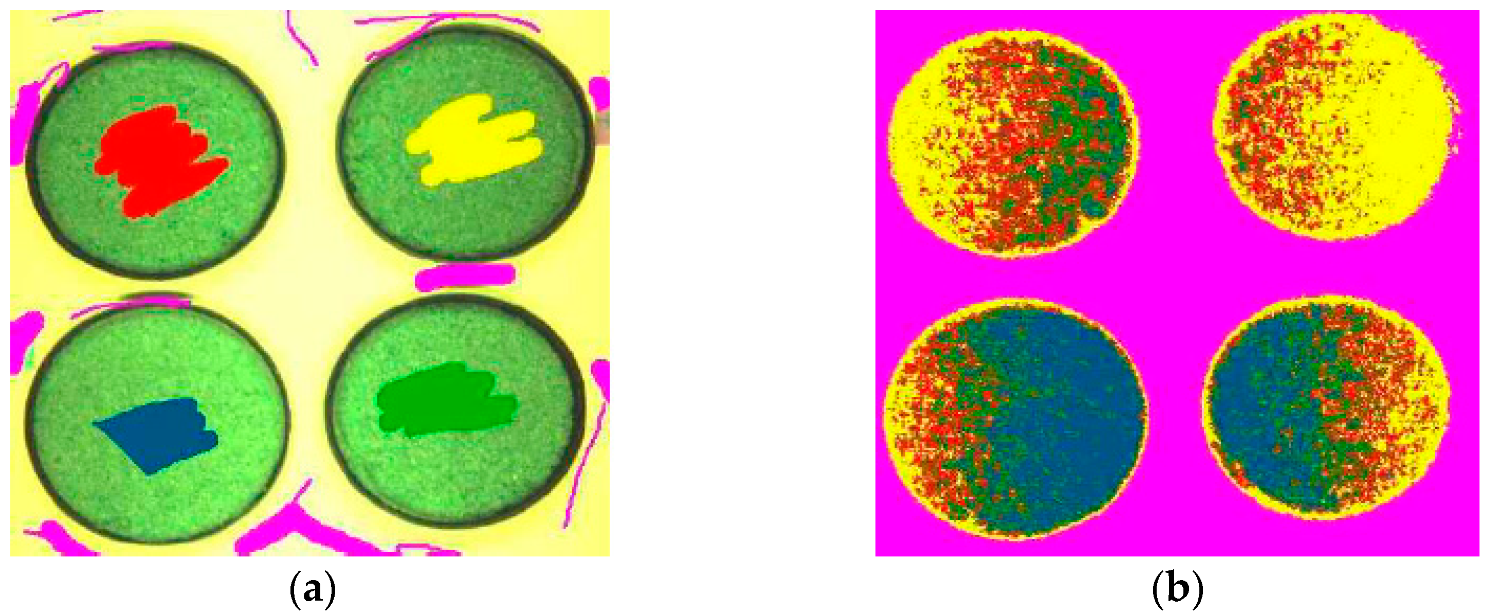
2.3. Extraction Method of Hyperspectral Information

Because spectral information includes reflectance over tens-to-hundreds of wavelength ranges, data preprocessing is essential to remove duplicate spectral information, wavelength noise, and other possible errors. Figure 5 shows the preprocessing performed in this study. After labeling the hyperspectral information as shown in Figure 5a, the distribution of the hyperspectral reflectance was obtained, as shown in Figure 5b. In this case, if diffuse reflection occurred owing to heterogeneity and variability in the process of the soil sample composition, the experiment was repeated.

3. Hyperspectral Information through Laboratory Tests

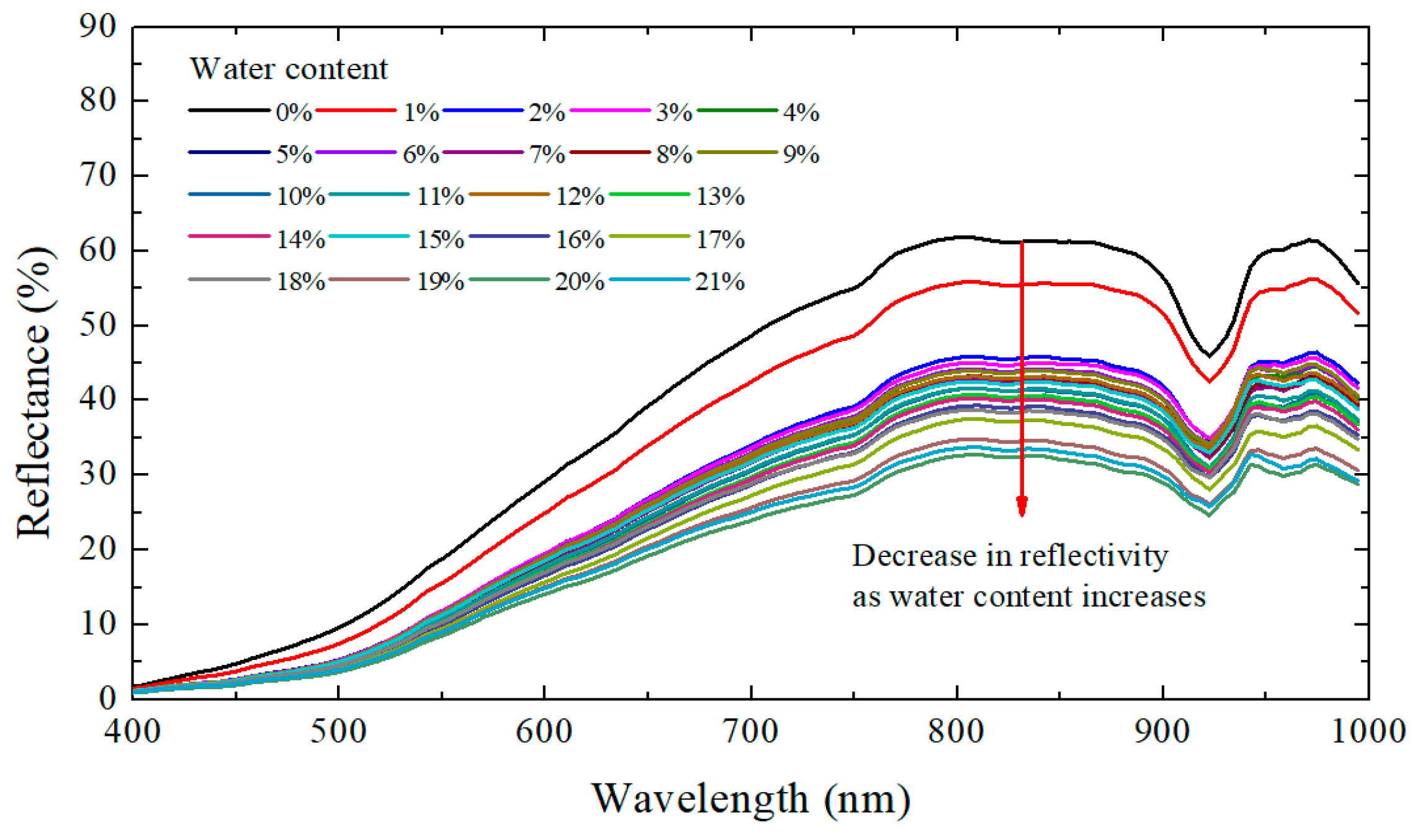
3.1. Relationshop between the Wavelength and the Reflection

In the case of soil with a water content of 22% or more, it behaved like a liquid and could not maintain a degree of compaction of 95%. In addition, in actual construction sites, compaction is not performed in soil containing too much water. Therefore, the test was not performed on soil with a water content of 22% or more.

The relationship between the wavelength and the reflectance under various water content conditions, derived through the experiments, is shown in Figure 6, in which 22 curves for the water content range from 0 to 21% are depicted. In all analysis cases, the curves of spectral information showed a similar nonlinear behavior. Up to a wavelength of 800 nm, where the maximum reflectance was measured, the reflectance was continuously increasing. Next, it decreased up to about a wavelength of 930 nm. Thereafter, the reflectance showed a rapid increase and, subsequently, a pattern of irregular decrease.

As the water content was increased, the reflectance decreased for the same wavelength. However, specimens with a water content of 1% or less exhibited relatively large reflectance values compared to specimens with other water content values. In addition, the wavelength–reflectance curves are similar at water contents of 11% to 19%, but the difference was small. Therefore, it was judged that careful classification of the corresponding range should be performed during the normalization process using the spectrum index. This is because, if the normalization of the corresponding range is not properly performed, a large error may occur in the prediction of water content based on the measured spectral information.

3.2. Spectrum Index for Normalization from the Literature

The spectrum index refers to a value obtained by converting spectral information (wavelength–reflectance curve), obtained through the experiments, into a single value and is normalized according to necessary information. In this study, the necessary information was water content, and the spectrum index should represent water content either directly or indirectly.

In order to determine the applicability of the existing spectrum indices, a literature review was conducted, and the result is summarized in

Table 2. Spectrum index estimations from the literature.

Research	Spectrum Index
Ge et al. [27]	DI = R866 − R655	(1)
Ge et al. [27]	RI = R866/R655	(2)
Ge et al. [27]	NDI = (R866 − R655)/(R866 + R655)	(3)
Ge et al. [27]	PI = (R866 − 0.4404R655 − 0.3308)/(1 + 0.44012)1/2	(4)
Haboudane et al. [25]	NDVI = (R800 − R680)/(R800 + R680)	(5)
Tian et al. [26]	DVI = R800 − R680	(6)

R_i is the reflectance at the i-nm wavelength.

. The existing indices for soil water content measurement and prediction include the difference index (DI), ratio index (RI), normalized difference index (NDI), and product index (PI) proposed by Ge et al. [27] and are presented in Equations (1)–(4). Here, the spectrum indices were calculated using the reflectance values corresponding to wavelengths of 866 nm and 655 nm. In addition, because there is no equation for calculating the spectrum index related to water content measurement, the spectrum index related to water was additionally investigated. Therefore, the normalized difference vegetation index (NDVI) and the difference vegetation index (DVI) were identified from further literature search, expressed as in Equations (5) and (6). These indices are mainly used for analysis of chemical compositions and structures of plants [25,26]. Here, the spectrum indices were calculated using the reflectance values corresponding to wavelengths of 800 nm and 680 nm.

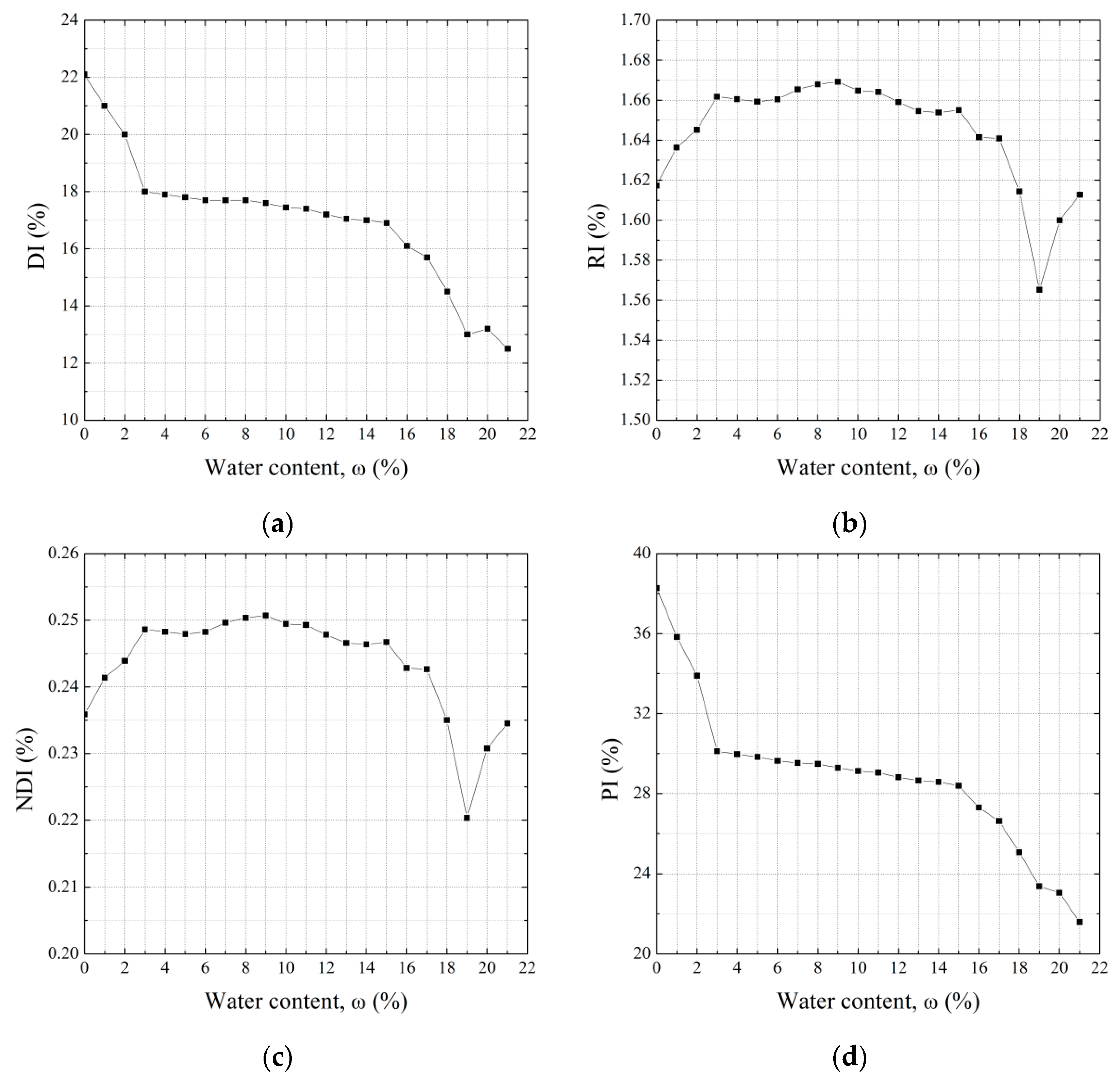
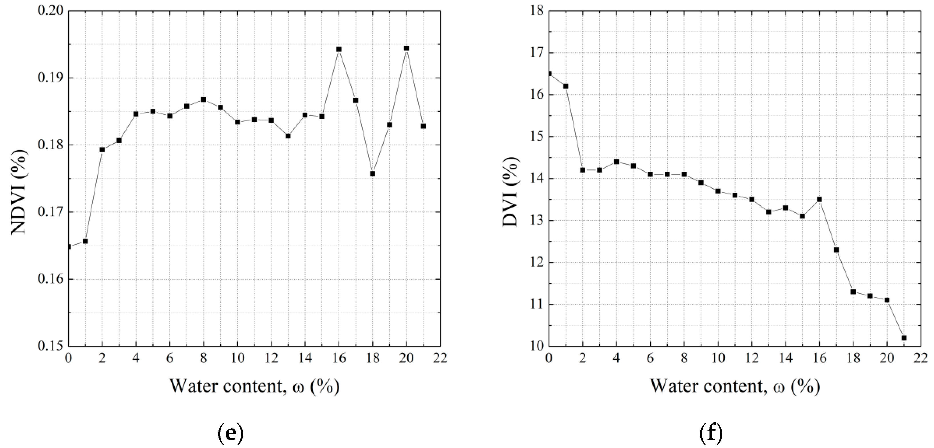
3.3. Calculation of the Spectrum Index

The calculation results of the spectrum indices according to Equations (1)–(6) in Table 2 are presented in Figure 7. The range of the values (value of the y-axis) reflected by each spectrum index was different, because the calculation methods are different. Therefore, a direct comparison of these values is meaningless. In terms of overall trends of the indices, DI, PI, and DVI showed similar patterns. The curves decreased sharply to a water content of about 3–4% and then showed a smooth decreasing trend. Subsequently, they decreased sharply again at a water content of about 15%. Additionally, the RI and the NDI were similar. These spectrum indices increased rapidly to a water content of about 3% and then showed a smooth upward convex parabolic shape. The indices increased, after a water content of 19% was used. The NDVI seemed to show a similar pattern to the RI or the NDI, but on the whole, showed an irregular pattern with a number of values out of the trend.

Except for the NDVI (irregular trend) and the DVI (outlier at a water content of 16%), the values of the DI, the RI, the NDI, and the PI showing specific trends, the DI and the PI showed a decreasing trend with the increasing water content, and the RI and the NDI showed a convex parabola shape. At this time, the RI and the NDI showing a parabolic shape were judged to be inappropriate. This is because for the calculation of a single spectrum index, two predicted water content values match the spectrum index. Therefore, among spectrum indices from the literature, only the DI and the PI should be used for comparisons, and the PI showed the most suitable characteristics.

4. Development of a New Spectrum Index for Water Content Prediction

4.1. Export of Specific Reflection for the Development of a New Spectrum Index

Among the spectrum indices from the literature, the PI was determined to be the most appropriate index for predicting water content. After calculating the PI (Equation (4)) from hyperspectral information, the wavelength–reflectance curve and the calculated spectrum index can be matched with the specific water content values on a one-to-one basis. This indicates that the water content can be predicted when the experimental procedure used in this study is applied to the ground with an unknown water content.

However, in the equation above, reflectances corresponding to wavelengths of 800 nm and 680 nm were used. Considering that 800 nm was the maximum measured reflectance in the wavelength–reflectance relationship shown in Figure 6, the reflectance corresponding to 680 nm had no significant characteristics. This indicated a lack of reliability in calculating the spectrum index.

Therefore, in this study, a new spectrum index that could be matched with water content one-to-one was calculated, and specific inflection point data shown in Figure 6 were extracted. At this time, the locations of the extracted data were all related to points with a significant change in the spectrum curves. The first inflection point (wavelength at 750 nm), the point of the maximum measured reflectance (800 nm), and the second inflection point (wavelength at 920 nm) are illustrated in Figure 8.

Figure 9 shows the reflectance versus the water content extracted from Figure 8. As the water content was increased, the reflectance showed a decreasing trend, and it can be seen that the trends for 0 and 1% water content values were somewhat different. The extracted trends according to the reflectance for each wavelength range were similar, which confirmed that determining the spectrum index by combining each reflectance did not have a significant meaning.

4.2. Fitting of Data for a Suitable Equation of the Spectrum Index

Data fitting was performed to determine an appropriate equation for spectrum index calculation. The final results are presented by converting the x-axis and y-axis of Figure 9 to those shown in Figure 10, considering that the input value is reflectance and the output value is water content. In this process, the reflectances at water contents of 0% and 1% were somewhat out of the trend and thus were excluded. Figure 10 shows that the water content gradually decreased as the reflectance increased, but it does not show a linear relationship. Therefore, a nonlinear equation for the relationship should be derived.

Various fitting equations (linear, polynomial, logarithm, exponential, and slogistic) were substituted for Figure 11, and the results are shown in Figure 12 and

Table 3. Results of fitting.

Point	Fitting Model	Equation	R2
1st inflection	Linear	$\mathsf{\omega }=-1.47+64.50$	0.837
	Polynomial	$\mathsf{\omega }=-0.001{\mathrm{R}}^4+0.11{\mathrm{R}}^3-4.73{\mathrm{R}}^2+88.16\mathrm{R}-576.89$	0.994
	Logarithm	$\mathsf{\omega }=-614.10\ln \left(\mathrm{R}+384.27\right)+3721.25$	0.858
	Exponential	$\mathsf{\omega }=-0.000788\exp \left(-\mathrm{R}/\left(-3.97\right)\right)+20.98$	0.991
	Slogistic	$\mathsf{\omega }=19.28/\left(1+\exp \left(0.63\left(\mathrm{R}-37.75\right)\right)\right)$	0.968
Maximum inflection	Linear	$\mathsf{\omega }=-1.34\mathrm{R}+67.67$	0.846
	Polynomial	$\mathsf{\omega }=-0.001{\mathrm{R}}^4-0.22{\mathrm{R}}^3+13.95{\mathrm{R}}^2-383.66\mathrm{R}+3932$	0.989
	Logarithm	$\mathsf{\omega }=-625.52\ln \left(\mathrm{R}+429.79\right)+3862.61$	0.833
	Exponential	$\mathsf{\omega }=-0.000487\exp \left(-\mathrm{R}/\left(-4.38\right)\right)+21.24$	0.986
	Slogistic	$\mathsf{\omega }=19.06/\left(1+\exp \left(0.68\left(\mathrm{R}-44.01\right)\right)\right)$	0.977
2nd inflection	Linear	$\mathsf{\omega }=-1.65\mathrm{R}+65.00$	0.880
	Polynomial	$\mathsf{\omega }=-0.001{\mathrm{R}}^4+0.17{\mathrm{R}}^3-6.74{\mathrm{R}}^2+117.42\mathrm{R}-731.72$	0.995
	Logarithm	$\mathsf{\omega }=-617.69\ln \left(\mathrm{R}+344.09\right)+3674.95$	0.871
	Exponential	$\mathsf{\omega }=-0.00131\exp \left(-\mathrm{R}/\left(-3.76\right)\right)+21.20$	0.993
	Slogistic	$\mathsf{\omega }=19.38/\left(1+\exp \left(0.65\left(\mathrm{R}-33.90\right)\right)\right)$	0.970

. Relatively large R-square was measured in a polynomial fitting model and an exponential fitting model, which means that the reflection–water content curve is suitable for both models. However, the polynomial fitting model must use the 4th order or higher, which requires five coefficients. In addition, although it is not expressed in the polynomial equation of Table 3, there is a disadvantage that a very large number of decimal places must be known. When rounding to two decimal places, fitting is not suitable, and at least six digits are required. On the other hand, the exponential fitting model requires three coefficients in a relatively simple equation. Therefore, it was judged that it is more reasonable to use the exponential equation in terms of usability.

4.3. Equation Selection for Water Content Prediction

Statistical analysis was performed to determine an appropriate exponential equation for water content measurement among the equations presented in Table 3. In this case, the predicted value was calculated using fitting equations, and the actual value is the point value of Figure 10. However, the sample size was small, with only 20 measured values, which may cause uncertainties of a significantly large error or a small error in the statistical analysis process. Therefore, the measured values were additionally set by dividing the interval between each point into 10 equal parts, assuming that the division between each point was linear.

Finally, the result of the comparison between the measured and predicted values (water content) with reflectance as the input value is shown in Figure 10. In addition, to quantify the comparative data in Figure 12, the R-square value, the mean and standard deviation of the bias factor (predicted value/measured value), and the coefficient of variation (COV) are listed in

Table 4. Comparison of bias factors of each inflection points.

Model of Curve	Inflection Point	Bias Factor
		R-Square	Average	St. Dev.	COV (%)
Exponential	1st	0.9924	1.010	0.066	6.554
	Maximum	0.9872	0.992	0.158	15.956
	2nd	0.9939	1.029	0.094	9.100

. As a result of the analysis, it was confirmed that the measured and predicted water contents showed the most linear relationship when the second inflection point was used. Further, the average of the bias factor was closest to 1, and the COV was the smallest at the first inflection point.

5. Conclusions

In the road construction process, for the quality of the road surface, compaction of the subgrade must be performed, and the water content of the ground must be understood for the degree of compaction. In this study, we tried to predict the water content based on hyperspectral information rather than the traditional water content measurement. However, as a result of examining the prediction methods of water content according to the existing literature, the equations in the existing literature were not suitable for water content prediction.

Therefore, we proposed an equation for prediction of water content according to the reflectance in a specific wavelength range, based on hyperspectral information (wavelength–reflectance curves), for different water content values. The key findings are outlined as follows:

(1)

In the existing literature, various spectrum indices for prediction of water content have been proposed. However, when the spectrum information obtained in this study was substituted into the equations for the spectrum index, it was confirmed that direct use is impossible, such as overlapping values and parabola curve. This is because the equation in the literature itself has great uncertainty and various conditions (indoor and outdoor, focal length, pixel width, etc.) exist in the process of acquiring hyperspectral information. Therefore, the reliability of the existing equation should be viewed as low. An optimized equation for prediction of water content should be selected by comparing it with the experimental results.

(2)

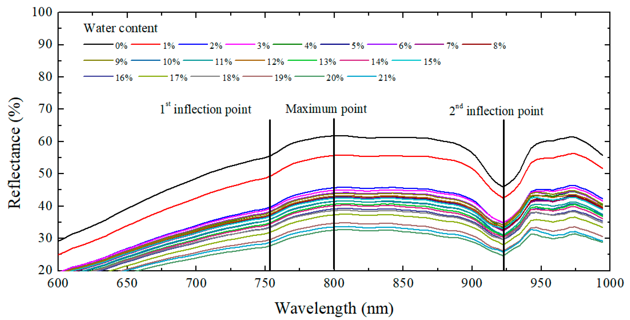
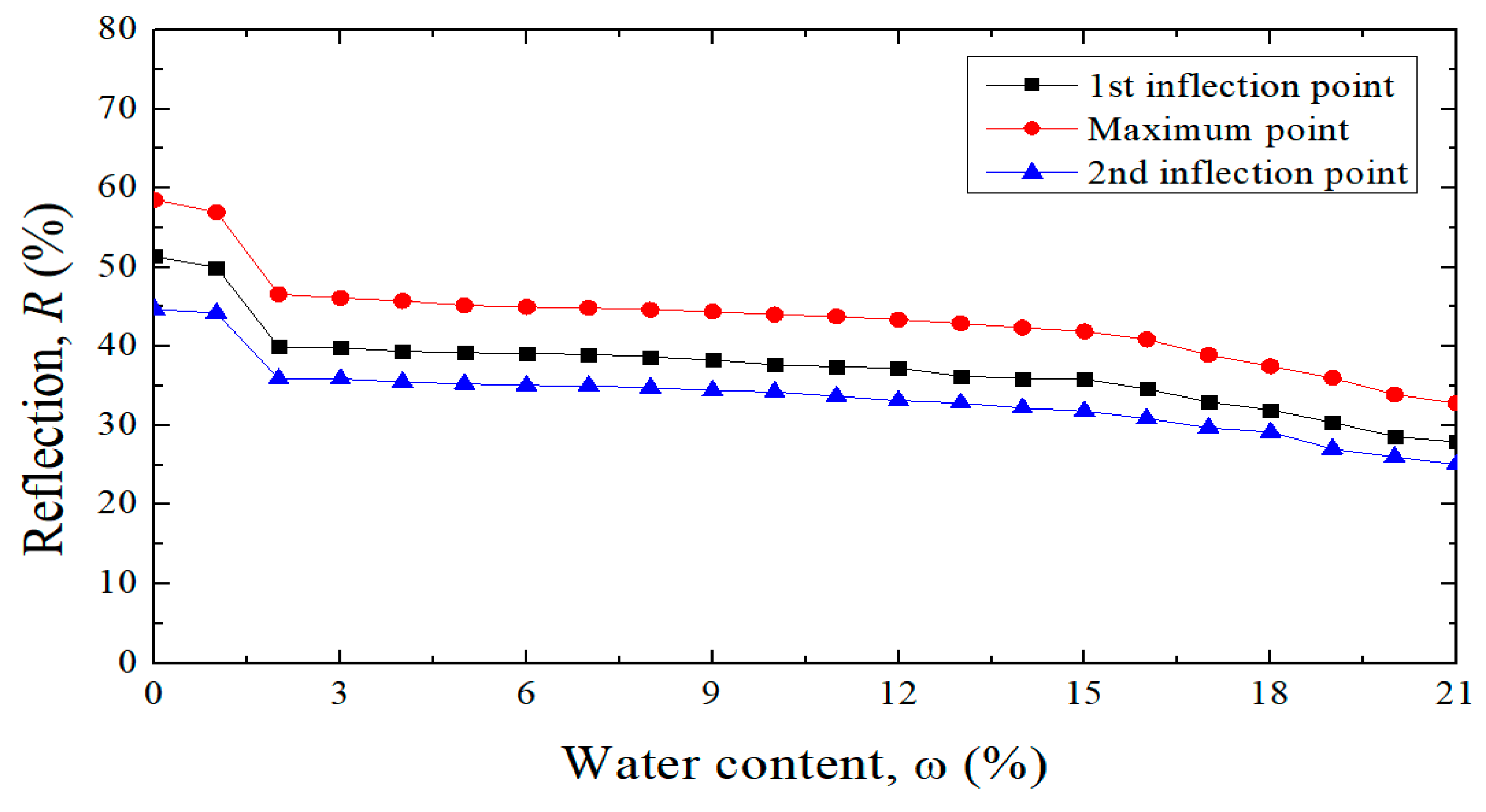
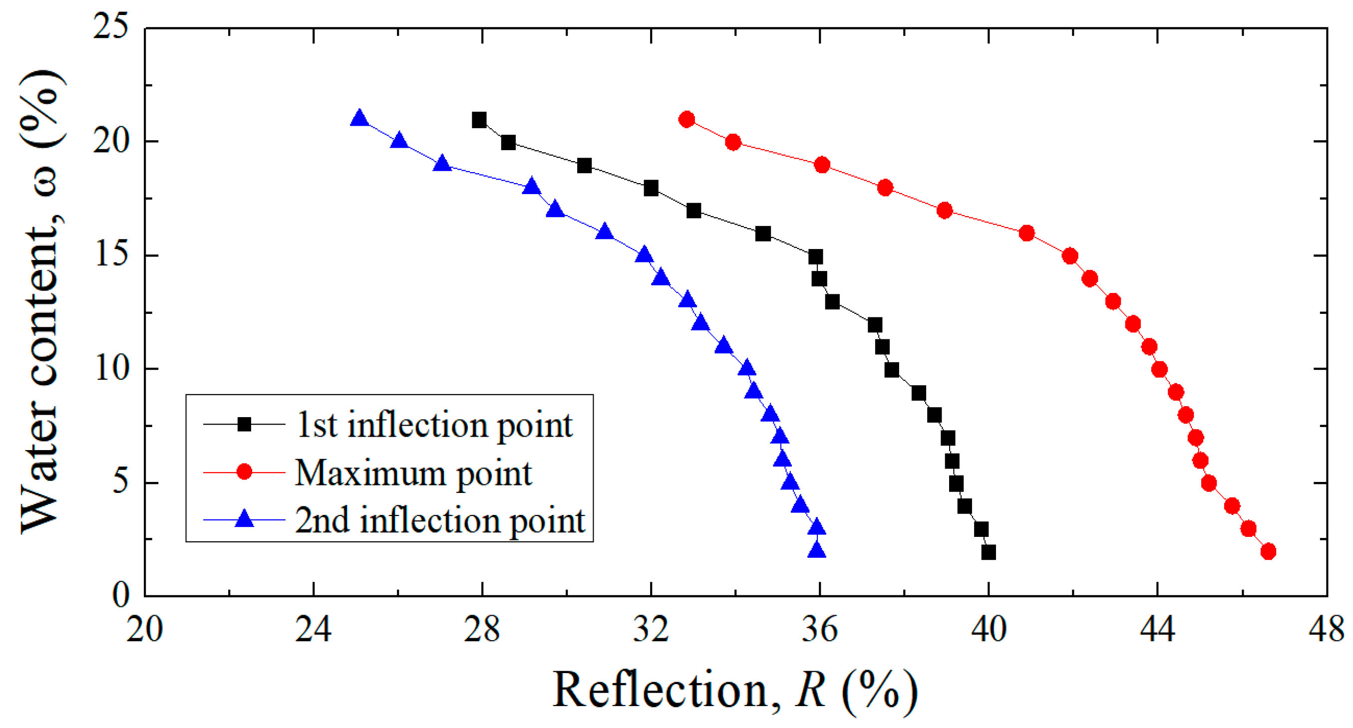
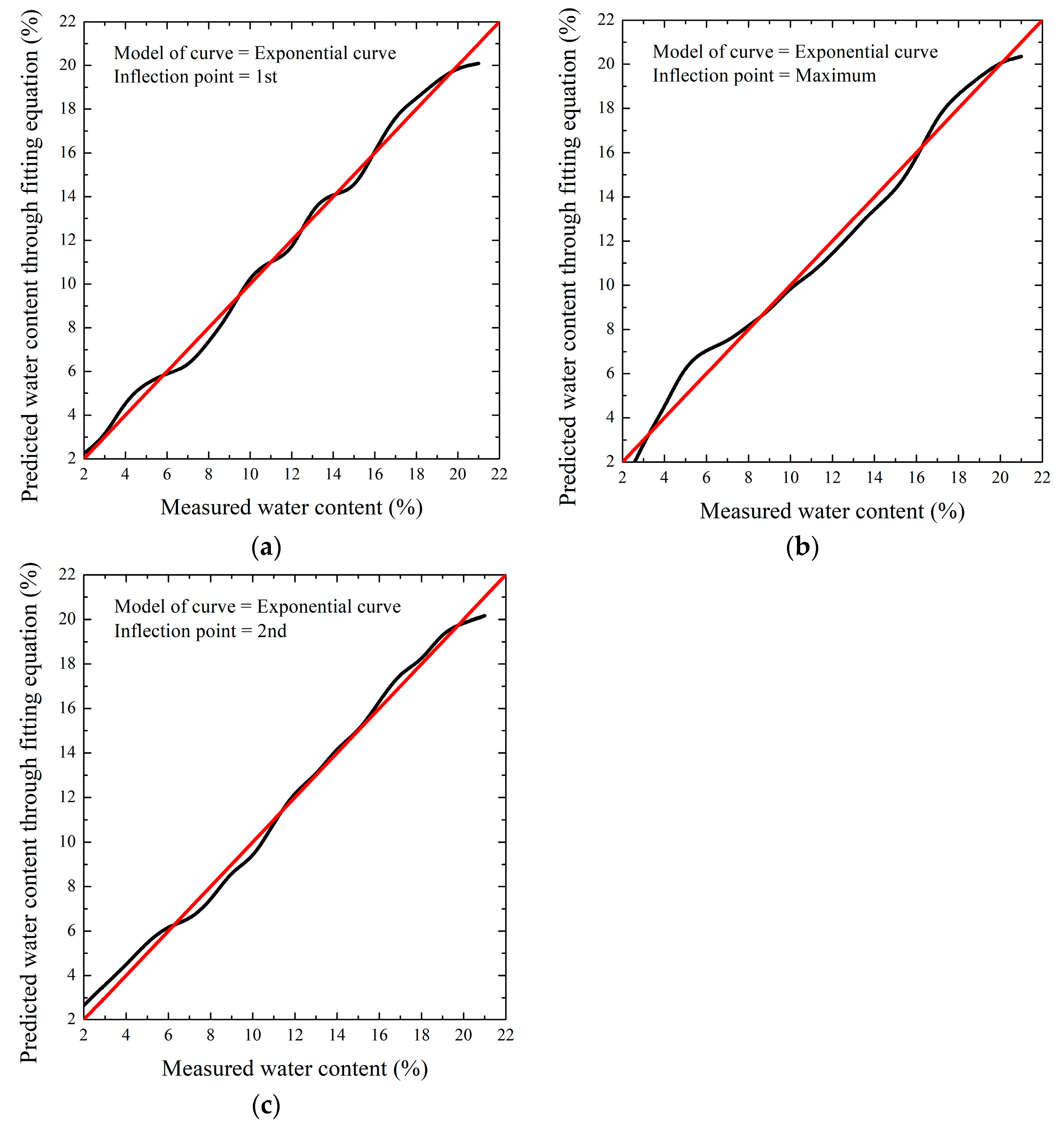
The prediction equation of water content may change, depending on the wavelength. However, the relationship between the wavelength and the curve used in the existing theory could not be confirmed. It was judged that it would be appropriate to extract a significant point from the wavelength−reflectance curve. Therefore, significant points were derived at the first inflection point (wavelength at 750 nm), the point of the maximum reflectance measurement (800 nm), and the second inflection point (wavelength at 920 nm). The first inflection point was a visible region in the wavelength band and corresponded to a deep red color. The maximum and second inflection points were near-infrared rays (NIRs), which cannot be seen by the human eye. The wavelength used for the final prediction equation of water content was the first inflection point, and it was judged that the wavelength selection in the visible region would be appropriate.

(3)

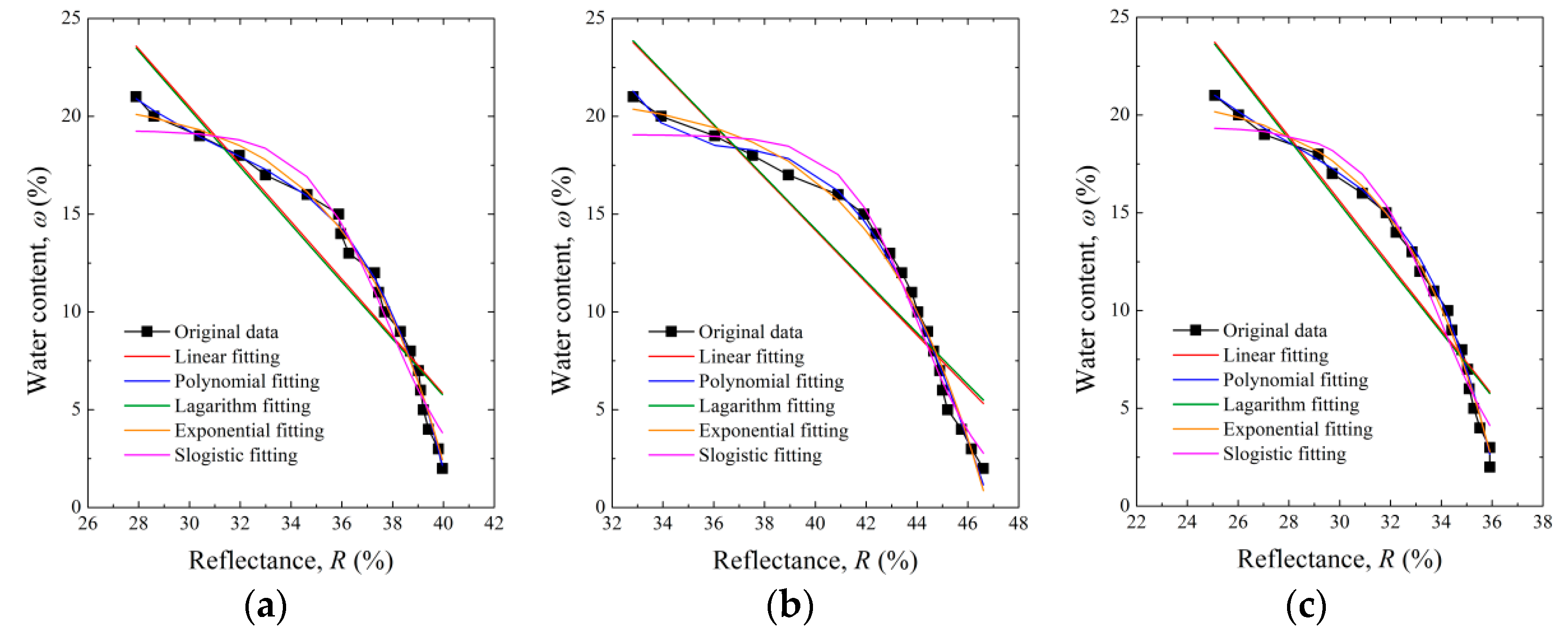
Through the comparison of various function models, the exponential equation was selected as a suitable model, and each extraction point was compared. In addition to R-square indicating linear regression, the COV of the bias factor indicating the occurrence of error also needs to be considered. This is because the reflectance for each wavelength range has a dense range of distribution according to water content, so that the occurrence of error greatly affects the output value (water content).

(4)

The hyperspectral information was obtained through precise laboratory tests on standard sand in this study. The equation for converting hyperspectral information into water content was proposed. This has the disadvantage that it was derived without performing various samples and field tests. It is meaningful in that it basically normalizes the water content prediction and proposes a new prediction equation of water content using hyperspectral information.

(5)

The subgrade soil of a real road construction site is not simply sand but a composite of various particle sizes, and errors may occur when the water content prediction formula developed in this study is applied. Thus, the accuracy and reliability of the derived equation should be tested and confirmed. If an error occurs in the application to real ground, the developed equation for prediction should be modified with a more comprehensive selection of soil types. Therefore, in future research, we aim to derive a specific wavelength range and reflectance in which a difference occurs ac-cording to water content, rather than being affected by the type of soil. Consequently, the equation derived above will be further modified and supplemented.

References

1. Kim, M.; Cho, Y. Evolution of corporate social contribution activities in the era of the Fourth industrial revolution. J. Korea Acad.-Ind. Coop. Soc. 2019, 20, 85–95. (In Korean) [Google Scholar]
2. Hong, S.; Chung, T.; Park, J.; Shin, H.S. Research on development of construction spatial information technology, using rover’s camera system. J. Korea Acad.-Ind. Coop. Soc. 2019, 20, 630–637. (In Korean) [Google Scholar]
3. Park, J.K.; Lee, K.W. Efficiency Analysis of Construction Automation Using 3D Geospatial Information. Sens. Mater. 2022, 34, 415–425. [Google Scholar] [CrossRef]
4. Seo, J.W.; Gang, T.G.; Choe, C.H. [I Priority sector] Automation Technology and Control Technology of Construction Equipment. Constr. Eng. Manag. 2020, 21, 4–10. [Google Scholar]
5. Sim, C.S.; Lee, S.Y.; Sim, S.H. [II Priority sector] Smart Construction Technology of road structures. Constr. Eng. Manag. 2020, 21, 11–15. [Google Scholar]
6. Ma, Y.; Luan, Y.C.; Zhang, W.G.; Zhang, Y.Q. Numerical simulation of intelligent compaction for subgrade construction. J. Cent. South Univ. 2020, 27, 2173–2184. [Google Scholar] [CrossRef]
7. ASTM D698; Standard Test Methods for Laboratory Compaction Characteristics of Soil Using Standard Effort (12,400 ft-lbf/ft3 (600 kN-m/m3)). American Society for Testing of Materials: West Conshohocken, PA, USA, 2017.
8. Roodposhti, H.R.; Hafizi, M.K.; Kermani, M.R.S.; Nik, M.R.G. Electrical resistivity method for water content and compaction evaluation, a laboratory test on construction material. J. Appl. Geophys. 2019, 168, 49–58. [Google Scholar] [CrossRef]
9. Ahmed, H.A. Electrical Resistivity Method for Water Content Characterization of Unsaturated Clay Soil. Ph.D. Thesis, Durham University, Durham, UK, 2014. [Google Scholar]
10. Abdullah, N.H.H.; Kuan, N.W.; Ibrahim, A.; Ismail, B.N.; Majid, M.R.A.; Ramli, R.; Mansor, N.S. Determination of soil water content using time domain reflectometer (TDR) for clayey soil. In Proceedings of the AIP Conference Proceedings, Penang, Malaysia, 5 October 2018. [Google Scholar]
11. Klotzsche, A.; Jonard, F.; Looms, M.C.; van der Kruk, J.; Huisman, J.A. Measuring soil water content with ground penetrating radar: A decade of progress. Vadose Zone J. 2018, 17, 1–9. [Google Scholar] [CrossRef]
12. Wen, M.M.; Liu, G.; Horton, R.; Noborio, K. An in situ probe-spacing-correction thermo-TDR sensor to measure soil water content accurately. Eur. J. Soil Sci. 2018, 69, 1030–1034. [Google Scholar] [CrossRef]
13. Peng, W.; Lu, Y.; Xie, X.; Ren, T.; Horton, R. An improved thermo-TDR technique for monitoring soil thermal properties, water content, bulk density, and porosity. Vadose Zone J. 2019, 18, 1–9. [Google Scholar] [CrossRef]
14. Ercoli, M.; Di Matteo, L.; Pauselli, C.; Mancinelli, P.; Frapiccini, S.; Talegalli, L.; Cannata, A. Integrated GPR and laboratory water content measures of sandy soils: From laboratory to field scale. Constr. Build. Mater. 2018, 159, 734–744. [Google Scholar] [CrossRef]
15. Zhou, L.; Yu, D.; Wang, Z.; Wang, X. Soil water content estimation using high-frequency ground penetrating radar. Water 2019, 11, 1036. [Google Scholar] [CrossRef]
16. Van der Meer, F. Imaging Spectrometry-Basic Principles and Prospective Applications; Kluwer Academic Publishers: Dordrecht, The Netherlands, 2003. [Google Scholar]
17. Bassani, C.; Cavalli, R.M.; Cavalcante, F.; Cuomo, V.; Palombo, A.; Pascucci, S.; Pignatti, S. Deterioration status of asbestos-cement roofing sheets assessed by analyzing hyperspectral data. Remote Sens. Environ. 2007, 109, 361–378. [Google Scholar] [CrossRef]
18. Smith, M.L.; Ollinger, S.V.; Martin, M.E.; Aber, J.D.; Hallett, R.A.; Goodale, C.L. Direct estimation of aboveground forest productivity through hyperspectral remote sensing of canopy nitrogen. Ecol. Appl. 2002, 12, 1286–1302. [Google Scholar] [CrossRef]
19. Kokaly, R.F.; Asner, G.P.; Ollinger, S.V.; Martin, M.E.; Wessman, C.A. Characterizing canopy biochemistry from imaging spectroscopy and its application to ecosystem studies. Remote Sens. Environ. 2009, 113, S78–S91. [Google Scholar] [CrossRef]
20. Zhang, F.; Zhou, G.S. Research progress on monitoring vegetation water content by using hyperspectral remote sensing. Chin. J. Plant Ecol. 2018, 42, 517. [Google Scholar]
21. Zhang, F.; Zhou, G. Estimation of vegetation water content using hyperspectral vegetation indices: A comparison of crop water indicators in response to water stress treatments for summer maize. BMC Ecol. 2019, 19, 18. [Google Scholar] [CrossRef]
22. Kovar, M.; Brestic, M.; Sytar, O.; Barek, V.; Hauptvogel, P.; Zivcak, M. Evaluation of hyperspectral reflectance parameters to assess the leaf water content in soybean. Water 2019, 11, 443. [Google Scholar] [CrossRef]
23. Aasen, H.; Burkart, A.; Bolten, A.; Bareth, G. Generating 3D hyperspectral information with lightweight UAV snapshot cameras for vegetation monitoring: From camera calibration to quality assurance. ISPRS J. Photogramm. Remote Sens. 2015, 108, 245–259. [Google Scholar] [CrossRef]
24. Eismann, M.T.; Stocker, A.D.; Nasrabadi, N.M. Automated hyperspectral cueing for civilian search and rescue. Proc. IEEE 2009, 97, 1031–1055. [Google Scholar] [CrossRef]
25. Haboudane, D.; Miller, J.R.; Pattey, E.; Zarco-Tejada, P.Z.; Strachan, I.B. Hyperspectral vegetation indices and novel algorithms for predicting green LAI of crop canopies: Modeling and validation in the context of precision agriculture. Remote Sens. Environ. 2004, 90, 337–352. [Google Scholar] [CrossRef]
26. Tian, Y.; Yao, X.; Yang, J.; Cao, W.; Zhu, Y. Extracting red edge position parameters from ground and space-based hyperspectral data for estimation of canopy leaf nitrogen concentration in rice. Plant Prod. Sci. 2011, 14, 270–281. [Google Scholar] [CrossRef]
27. Ge, X.; Wang, J.; Ding, J.; Cao, X.; Zhang, Z.; Liu, J.; Li, X. Combining UAV-based hyperspectral imagery and machine learning algorithms for soil moisture content monitoring. PeerJ 2019, 6926, e6926. [Google Scholar] [CrossRef]
28. ASTM D422; Standard Test Method for Particle-Size Analysis of Soils. American Society for Testing of Materials: West Conshohocken, PA, USA, 2016.
29. ISO 679; Cement-Test Methods-Determination of Strength. International Organization for Standardization: Geneva, Switzerland, 2009.
30. ASTM D2487; Standard Practice for Classification of Soils for Engineering Purposes (Unified Soil Classification System). American Society for Testing of Materials: West Conshohocken, PA, USA, 2017.
31. Lu, G.; Fei, B. Medical hyperspectral imaging: A review. J. Biomed. Opt. 2014, 19, 010901. [Google Scholar] [CrossRef] [PubMed]
32. Ortega, S.; Guerra, R.; Diaz, M.; Fabelo, H.; López, S.; Callico, G.M.; Sarmiento, R. Hyperspectral Push-Broom Microscope Development and Characterization. IEEE Access 2019, 7, 122473–122491. [Google Scholar] [CrossRef]
33. Habib, A.; Zhou, T.; Masjedi, A.; Zhang, Z.; Flatt, J.E.; Crawford, M. Boresight calibration of GNSS/INS-assisted push-broom hyperspectral scanners on UAV platforms. IEEE J. Sel. Top. Appl. Earth Obs. Remote Sens. 2018, 11, 1734–1749. [Google Scholar] [CrossRef]
34. Horstrand, P.; Díaz, M.; Guerra, R.; López, S.; López, J.F. A novel hyperspectral anomaly detection algorithm for real-time applications with push-broom sensors. IEEE J. Sel. Top. Appl. Earth Obs. Remote Sens. 2019, 12, 4787–4797. [Google Scholar] [CrossRef]
35. Angel, Y.; Turner, D.; Parkes, S.; Malbeteau, Y.; Lucieer, A.; McCabe, M.F. Automated georectification and mosaicking of UAV-based hyperspectral imagery from push-broom sensors. Remote Sens. 2020, 12, 34. [Google Scholar] [CrossRef]
36. Jurado, J.M.; Pádua, L.; Hruška, J.; Feito, F.R.; Sousa, J.J. An Efficient Method for Generating UAV-Based Hyperspectral Mosaics Using Push-Broom Sensors. IEEE J. Sel. Top. Appl. Earth Obs. Remote Sens. 2021, 14, 6515–6531. [Google Scholar]
37. Yi, L.; Chen, J.M.; Zhang, G.; Xu, X.; Ming, X.; Guo, W. Seamless Mosaicking of UAV-Based Push-Broom Hyperspectral Images for Environment Monitoring. Remote Sens. 2021, 13, 4720. [Google Scholar] [CrossRef]
Figure 1. Material properties of the sand used in this study: (a) particle size distribution curves of the used sand and the standard sand]; (b) compaction curve as a function of water content.
Sustainability 14 10999 g001
Figure 2. Analysis system for obtaining the hyperspectral information of soil: (a) combination of each device; (b) photo.
Sustainability 14 10999 g002
Figure 3. Push-broom scanning method: (a) application using a flight vehicle; (b) application in this study (laboratory test).
Sustainability 14 10999 g003
Figure 4. Experimental process to obtain hyperspectral information about the water content: (a) mixing of a sample soil with standard sand and water; (b) composition of the specimen in circular petri; (c) scanning after setting on the stage with the push-broom method; and (d) confirmation and analysis of hyperspectral information using software.
Sustainability 14 10999 g004
Figure 5. Image preprocessing process: (a) labelling of hyperspectral information; (b) distribution of hyperspectral reflection.
Sustainability 14 10999 g005
Figure 6. Relationships between the wavelength and the reflectance for different water content values.
Sustainability 14 10999 g006
Figure 7. Spectrum indices versus water content from the literature: (a) DI; (b) RI; (c) NDI; (d) PI; (e) NDVI; and (f) DVI.
Sustainability 14 10999 g007aSustainability 14 10999 g007b
Figure 8. Export of specific reflection with the changing of curves.
Sustainability 14 10999 g008
Figure 9. Reflectance versus water content at inflections and maximum points.
Sustainability 14 10999 g009
Figure 10. Transformation of the x- and y-axes of Figure 9.
Sustainability 14 10999 g010
Figure 11. Results of substituting various fitting equations: (a) at the 1st inflection point; (b) at the maximum point; and (c) at the 2nd inflection point.
Sustainability 14 10999 g011
Figure 12. Comparison between the measured and predicted water contents: (a) at the first inflection point; (b) at the maximum inflection point; and (c) at the second inflection point.
Sustainability 14 10999 g012