Evolutionary Participatory Selection for Organic Heterogeneous Material: A Case Study with Ox-Heart Tomato in Italy

Abstract

Cultivars specifically adapted to organic agriculture are lacking in most crops, and tomato is no exception. Evolutionary-participatory breeding (EPB) combines the adaptive ability of evolutionary populations with farmers’ selection, thus representing a cost-effective strategy for the development of novel organic heterogeneous material, as introduced by the European regulation on organic agriculture (EU) 2018/848. An F4 ox-heart tomato composite cross population (CCP), derived from a half-diallel cross of four local varieties chosen for their superior performance under organic conditions, was submitted to both natural and farmers’ selection on three organic farms and at one research station in Italy. During field days held at each location before harvest, farmers visually scored 400 plants, all of which were carried forward to develop the natural selection (NS) population, while the 20 best ranking plants were chosen to develop the farmers’ selection (FS). After two cycles of selection (2018 and 2019), one NS and one FS population were obtained at each location. After this two-year selection process, in 2020, the eight populations (four NS and four FS), were evaluated in a randomised complete block trial in the four locations of selection and evolution. Four local varieties chosen by farmers and two modern varieties (one open pollinated variety and one F₁ hybrid) were added as controls. The ANOVA showed significant differences among entries for all traits. Entry-by-location interactions were larger than the genetic effect for the overall evaluation, yield at first harvest, total yield and percentage of marketable yield. This confirms the importance of decentralising selection when seeking to develop specifically adapted varieties and/or populations. Evidence was observed of the effectiveness of participatory selection for improving the yield at first harvest, with a slight trade-off effect for the total yield and plant vigour.

1. Introduction

It has been widely recognised that intensive agriculture is unsustainable in terms of resource use efficiency and has outstepped planetary boundaries with relation to nitrogen use and biodiversity loss [1,2]. Agro-ecological and organic systems offer a viable alternative without compromising long-term food security [3]. However, the lack of suitable cultivars is limiting their potential since more than 95% of organic production is based on crop varieties that were bred for conventional high-input systems [4].

Tomato (Solanum lycopersicum) is the seventh most grown crop in the world [5] and Italy is the largest tomato producer in Europe [6]. Despite being a secondary centre of diversification with a large number of local varieties [7], many of the cultivars presently grown in Italy have been bred outside of the country [8], and as for many other crops, intense genetic erosion has been documented [9,10,11]. Tomato breeding efforts over the past decades have been directed toward high-yielding F₁ hybrids at the expense of open pollinated varieties. Of the 588 tomato varieties registered on the Italian national variety list, only 72 are open pollinated (among which there are three conservation and three amateur varieties) [12]. This limits the adaptive potential of the crop to specific environments, organic management and climate change challenges [13,14]. A renewed interest in local tomato varieties started in the 1980s with the appearance of the Protected Designation of Origin quality scheme (the “San Marzano” tomato being the earliest variety to be protected in this way) [15], followed by the registration of several conservation and amateur varieties under the EU directive 2009/145/EC [16]. In this context, organic agriculture has played a significant role in the preservation and continuous evolution of landraces in many different crops, and tomato is no exception; the robustness and resilience of these varieties may largely explain their success [17,18,19]. Organic tomato cultivation has been growing significantly around the world, especially in the US [20] and Europe [21]. However, local tomato varieties still face limitations in terms of their yield, nutrient use efficiency and tolerance or resistance to pests and pathogens, which highlight the importance of specific breeding programs for organic conditions [4,22].

In Italy, despite the exponential growth of the organic sector in recent years (representing 15.8% of the cultivated area against a European average of 8% in 2020) [23], the number of derogations granted to use non-organic tomato seed has remained stable (from 4752 in 2018 to 4482 in 2020) [24]. This appears consistent with the findings of Solfanelli et al. [25], who reported a 70% use of non-organic tomato seed by organic farmers in Southern Europe. Breeding new cultivars for organic agriculture remains challenging from an economic point of view due to the constrained size of the organic seed market, combined with the widespread use of derogations by organic farmers [26], which limit the potential revenue from organic seed sales. Furthermore, varietal choice for organic Italian tomato growers is restricted by the fact that farmers tend to purchase tomato transplants from horticultural nurseries, hence delegating the varietal choice to the seed and fresh produce market.

One viable and cost-effective strategy for organic plant breeding is evolutionary participatory breeding (EPB), which combines the adaptation potential of evolutionary populations with structured decentralised participatory plant breeding (PPB) programmes [27,28,29]. This approach, pioneered by Harlan and Martini and by Suneson for cereal crops [30,31] in the first half of the 1900s, was successfully applied to tomato in Italy by Campanelli et al. [8,32]. In several other crops, a number of PPB programmes have led to improved selection efficiency and higher adoption rates [33,34,35]. A review by Colley et al. [36] of PPB initiatives in the Global North (United States, Canada and Europe) identified 47 such projects targeting a total of 22 crop species, mainly addressing the needs of organic farming systems.

From January 2022, the European regulation for organic agriculture (EU) 2018/848 introduced the possibility to notify, produce and certify seed of organic heterogeneous material, widening the scope of a successful experiment in Europe with cereal populations (2014/150/EU) to all crops [37]. This represents a tremendous opportunity to quickly and effectively develop new heterogeneous cultivars, adapted and adaptable to organic growing conditions and specific geographical regions.

In the present work, we describe an EPB programme targeting an ox-heart tomato population, as developed during the SOLIBAM European project (2010–2014 www.solibam.eu; accessed on 1 October 2020), where tomato was used as a model crop to create one of the first documented horticultural composite cross populations (CCPs), building on earlier successful initiatives with cereals [38]. The work on this tomato CCP continued with the European project LIVESEED (2017–2021 www.liveseed.eu; accessed on 1 June 2022), which aimed to enhance organic breeding and the use of organic seed. The SOLIBAM tomato CCP was grown at four locations in different Italian regions, where it was submitted to both farmers’ selection (FS) and natural selection (NS) for two years. In the third and final year, the populations from each environment (four FS and four NS) were tested in a multi-location trial (MLT) in the four locations of selection and evolution. The objective was to assess the efficiency and effectiveness of farmers’ visual selection within a CCP, compared to both existing varieties and the products of natural selection.

2. Materials and Methods

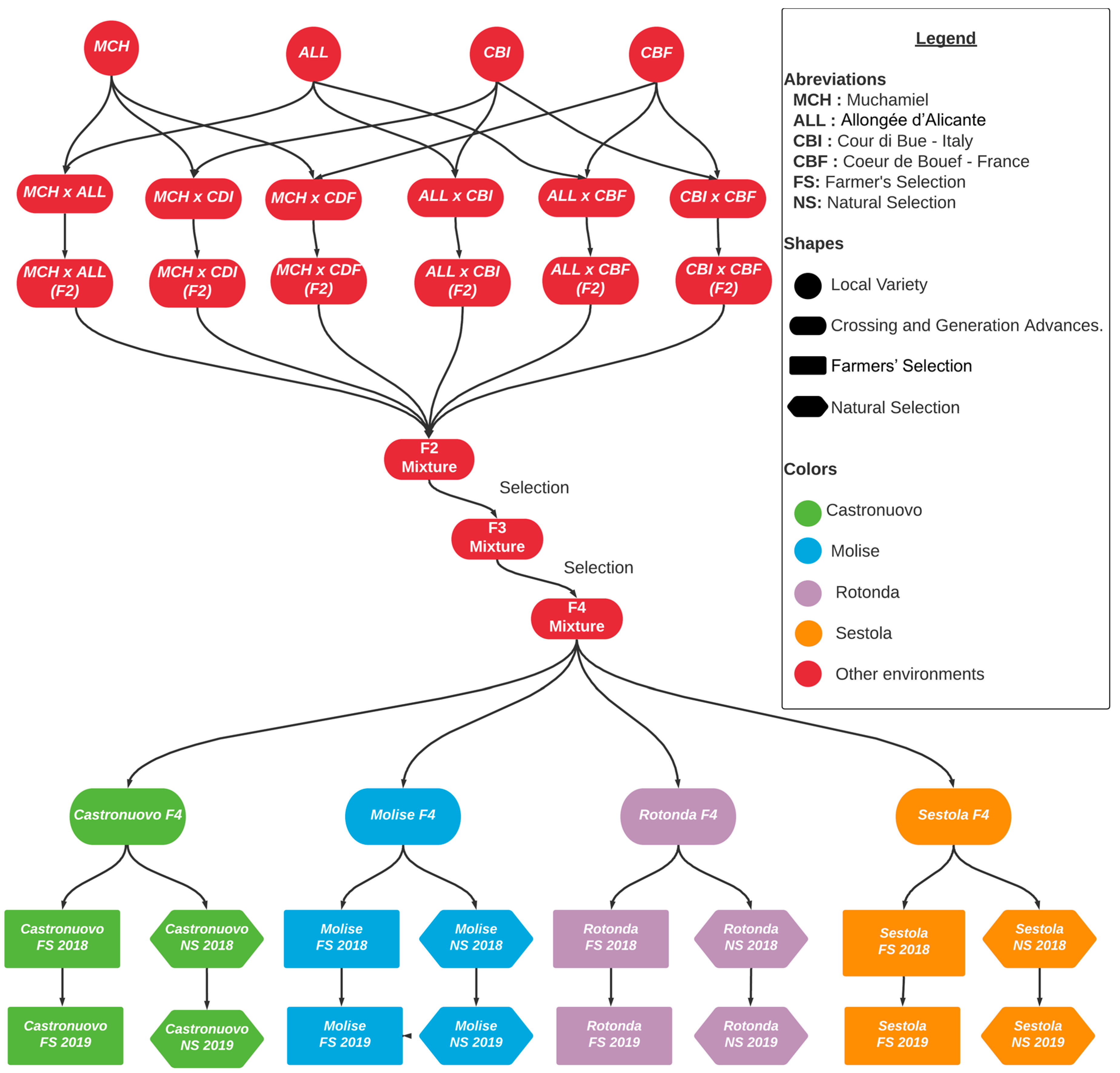
2.1. Plant Material

The tomato population used for this study was developed under the SOLIBAM European project, as part of which 35 tomato landraces were evaluated at four locations in France and Italy in 2011. Following a participatory evaluation, four varieties were selected by the French seed company Gautier Semences, according to key traits of interest for both direct use by organic farmers and for its own tomato breeding programme. The selection comprised two ox-heart types from France and Italy (Cuor di Bue and Cœur de Bœuf, respectively) and two Spanish landraces (the ribbed marmande-type Muchamiel and the smooth skinned Allongée d’Alicante) (

Table 1. Landraces used to form the tomato CCP.

Name	Allongée d’Alicante	Muchamiel	Cuor di Bue	Cœur de Bœuf
Origin	Spain	Spain	Italy	France
Shape	Rectangular	Marmande	Ox-Heart	Ox-Heart
Maturity	Late	Medium	Early	Medium
Growth Habit	Indeterminate	Determinate	Indeterminate	Indeterminate
Fruit weight (g)	150–190	190–250	190–250	190–250
Trait of interest	Homogeneity	Firmness	Shape	Shape

). The four varieties were crossed following a half-diallel scheme in 2012, producing six F₁ progenies. In the same year, these were grown in isolation and self-pollinated; the F₂ seed produced was mixed to constitute an evolutionary population [38,39].

Four hundred plants of this population were grown in 2013 at the organic farm Il Lombrico Felice (Perugia, Italy), then subjected to negative selection by Italian organic seed company Arcoiris to discard offtypes or plants with extreme susceptibility to disease. The resulting F₃ bulk was planted in 2014 at the Orti Corti farm (Santarcangelo di Romagna, Italy) and submitted to selection using the same criteria. The resulting harvest constituted the F₄ evolutionary population that was used as the starting material for the experiment described in this paper (Figure 1).

2.2. Trial Locations

The trials were held on organic farms at four different locations, representing diverse pedo-climatic conditions and management approaches (Figure 2). At three of the four locations, the project was implemented on the same farms over the three years. These were Alle Fontanine farm (Sestola, Emilia-Romagna), Silvano Di Leo’s farm (Castronuovo di Sant’Andrea, Basilicata) and the experimental farm A.A.S.D. Pollino of the regional agricultural agency ALSIA (Rotonda, Basilicata; www.alsia.it; accessed on 1 June 2022). In the case of the fourth location, in the Molise region, three different farms located within a 25 km radius were involved in different years: Vincenzo Battezzato’s farm (Campobasso, 2018 and 2019), Agribio Petacciato (San Giuliano di Puglia, 2019) and Primo Sole (Montagano, 2020).

2.3. Participatory Selection

In 2018, for each of the four locations, plots of 400 plants from the F₄ population were planted using the agronomic practices routinely applied on each farm involved. Right before the first harvest, a group mainly composed of farmers, but also researchers, technicians and citizens, was invited to the field and asked to evaluate each individual plant. Each participant was given a scoring form with a row for each of the 400 plants, and asked to independently choose a score for each individual plant (1 = not satisfying at all, 2 = unsatisfying, 3 = satisfying, 4 = very satisfying). Even though this exercise involved not just farmers, it was termed farmers’ selection for simplicity. All evaluations were averaged, and 20 seeds from each of the 20 best-ranking plants were taken to constitute the farmers’ selection population (FS) for the following year. At the same time, one random fruit from the first truss was collected from each of the 400 plants, and their seeds were mixed to constitute the natural selection population (NS) for the following year.

In 2019, at each location, the 400 plants of the FS populations were planted and evaluated in the same way as the previous year. On all farms, spatial arrangement consisted of 10 rows of 40 plants each, to allow for an even distribution of the 20 families of 20 individuals derived from each plant selected the previous year. Participatory evaluation was repeated as described for the first year, and a new FS population was formed for each location with 20 seeds from the 20 best-ranking plants. At the same time, 400 plants from the NS grown the previous year were planted, and the seeds from one random fruit per plant were collected to advance each NS population by one generation. After two growing seasons, four FS populations and four NS populations (one FS and one NS from each location) were obtained (Figure 1). In the case of Molise, in 2018, both FS and NS were obtained from Vincenzo Battezzato’s farm. In 2019, the FS was planted and selected on Vincenzo Battezzato’s farm, and the NS on Agribio Petacciato’s farm.

2.4. Multi-Location Trial

In 2020, a multi-location trial (MLT) was established at the four locations where selection had been conducted. In the case of Molise, the trial was conducted at the Primo Sole farm in Montagano, whereas at the other three locations, the trials were conducted on the same farms where the selection had taken place. All four farmers’ selection (FS) and all four natural selection (NS) populations were sent to each of the four locations. Additionally, one local variety (LV) to be used as the control was chosen by each farmer, with these four LVs added to the trials at each location. They were Costoluto di Parma (Arcoiris Sementi) for Sestola, Rosa di Castronuovo (farm-saved seed by Silvano di Leo) for Castronuovo, Miscuglio di Rotonda (ALSIA Pollino seed bank) for Rotonda and Kéro F₁ (seed provided by Primo Sole farm) for Molise. Two commercial controls were also included, the open pollinated variety (OPV) Belmonte (Sementi Biologici) and F₁ hybrid Déko (ISI Sementi), with a total of 14 entries across locations.

Trials were designed as randomised blocks in rows and columns with two replicates and 28 plots. Each plot consisted of 20 plants, subdivided into two adjacent rows of 10 plants each. The total number of rows per field was 14; each row had 40 plants and every pair of rows contained four plots. The distance was 1.5 m between rows and 20 to 40 cm between plants, depending on the farm (Figure 3). Independent randomisations for each farm were obtained with DiGGeR software, which produces non-factorial experimental designs for experiments arranged in rows and columns [40].

Yield data were collected from all four locations by the host farmers or local technicians. The plots were harvested over four different rounds, and for each of these, the date of harvest, number of plants harvested, number of fruits and total fruit weight were recorded. The yield was also divided into marketable and non-marketable harvests, according to the criteria of the corresponding farmers.

For each of the four locations, a group of participants (mostly farmers but also other actors) was invited to evaluate each plot. As previously described, evaluations were made on a scale of 1 to 4, with five parameters considered: (i) disease resistance, (ii) homogeneity, (iii) plant vigour, (iv) estimated yield and (v) overall evaluation. Each participant was given a score form with the plot numbers and asked to make their evaluations independently. The identity of each plot was revealed only after all evaluations were completed.

2.5. Statistical Analysis

Although all plots started with 20 plants, hailstorms and heavy rains reduced the plot stands, especially at Sestola where the plants per plot varied between 13 and 20 (mean of 15.9 ± 1.96). Therefore, the yield components were divided by the actual plot stand, to obtain the weight and number of fruits per plant. ANOVA was carried out through R and the Rstudio platform [41]. Although each FS and NS evaluated in 2020 was a mixture of F₆ individuals/genotypes with some expected levels of heterozygosity, they were treated as “heterogeneous materials” when compared to one another and versus local varieties and controls. For that reason, all entries evaluated at each location were considered a “genotype” in the ANOVA, meaning a total of fourteen genotypes per location (4 FS, 4 NS, 4LV and 2 controls) were considered in the analyses of variance.

Spatial analysis was performed to correct for the field heterogeneity and calculate the best linear unbiased estimators (BLUEs) for each entry at each location. This was done with the R package “SpATS”, which uses two-dimensional P-splines with anisotropic smoothing within the mixed model framework [42]. The model used is the following:

$$y=f\left(u,v\right)+Z_c{c}_c+Z_r{c}_r+X_g{\beta }_g+\varepsilon$$

where $y$ is the response variable and $f\left(u,v\right)$ is the “smooth-by-smooth interaction trend jointly defined over the row and column directions”. $Z_c{c}_c$ and $Z_r{c}_r$ correspond to the random effects of column and row, and their associated design matrices; $X_g{\beta }_g$ stands for the genotypic effect considered as fixed; $\varepsilon$ represents the error of the model [42]. The adjusted means (the sum of the BLUEs and the intercept) and the associated standard errors were used to plot the values for each genotype at each location. These values were also used to perform Tukey’s HSD mean comparison tests in each environment, to statistically separate the genotype means (α = 0.05).

The BLUEs’ values were then used to analyse the information through GGE biplots [43], executed through the R package “metan” [44]. A GGE biplot is a useful tool for the analysis of genetic and genotype × environment effects, where the PC1 (x-axis) is proportional to the former and the PC2 (y-axis) to the latter. The analysis is carried out on standardised values and plots centred around the environmental values. Two specific features of the GGE biplot were used in this case. The “which-won-where” type draws a polygon along the genotypes that are the farthest away from the origin; the genotypes with the longest vectors are thus the most responsive. Genotypes on the polygon vertex perform best at the locations found in the same sector [44]. The “mean vs. stability” feature draws a first line, the mean environmental axis, passing through the origin, with an arrow representing the “ideal” environment, and then a second line perpendicular to the first, which represents the G×E interaction. Genotypes with projections close to the arrow in the first axis are high performers in this ideal environment, while large projections on the second axis indicate low stability or high G×E interaction. For the specific case of this work, G×E interaction is interpreted only as genotype × location interaction, with “environments” as locations, since the trials were all carried out in one year.

Two main questions drove the analysis for the BLUEs data from the MLT: (i) was farmers’ selection effective for the evaluated traits? and, (ii) was there any evidence of local adaptation of the populations to the location where selection was conducted? Each of these questions had a specific comparison of interest (

Table 2. Research questions and comparisons of interest that drove the statistical analysis of the data from the tomato EPB project.

Research Question	Comparison of Interest
Was farmers’ selection effective for the evaluated traits?	Farmers’ selections vs. natural selections from the same location
Is there evidence of local adaptation in the populations to the location where selection occurred?	For each location, local vs. non-local natural and farmers’ selection populations

).

To better understand the changes between the FS and NS populations, a comparison of the yield components was carried out. In this way, the yield of each population at each location was dissected by time (the four different harvests), as well as by the mean fruit weight and fruit number. A two-sample t-test was run at every possible point of comparison.

Moreover, to identify correlations among the participants’ evaluations and the quantitative agronomic traits, Pearson’s correlation coefficient r was estimated for each pair of traits at the overall level, then at every location (data not shown). The quantitative traits included were the yield at first harvest, total yield, mean fruit weight, number of fruits per plant and percentage of marketable yield. The evaluations included were the overall evaluation, estimated yield, vigour, disease resistance and homogeneity. The overall evaluation was also disaggregated by gender. Additionally, a special mean for the overall evaluation was included, estimated only with the evaluations of consistent actors, that is, those actors who participated in 2020 and in at least another earlier evaluation cycle (2018 or 2019). Finally, a correlation plot was built with all the r coefficients and their corresponding significance levels, using the R package “metan” [43].

After comparing genotypes with individual variables, a multivariable analysis was carried out through a Principal component analysis (PCA). The PCA was performed at the location level, using the mean value of each genotype for each of the variables described in the correlation analysis. This was done using the R package “factoextra” with the default parameters [45].

3. Results

3.1. Climatic Data

Although temperature patterns across the locations and over the years were fairly similar, important differences in rainfall were observed (Figure 4). Castronuovo received high rainfall in August 2020, leading to severe flooding in the area, followed by a hailstorm, which severely damaged the crop. Days with extremely high rainfall were also observed in other locations in the same year, with Sestola reaching a record accumulated daily rainfall of 85 mm in July. The warmest location was Castronuovo, where the highest temperature recorded was 35 °C, whilst Sestola, the northernmost location and with the highest elevation, had the lowest temperatures through the growing seasons.

3.2. Participatory Selection and Evaluation

A range of diverse actors participated in this EPB project across the three years and the four locations. A total of 174 participants took part in the selections and evaluations at least once during the three years of trials: 75% were men and 25% women, whilst farmers comprised the largest group, accounting for 44% of total evaluators (Figure 5A). The consistency in participation across the years is shown in Figure 5B. In 2019, the percentage of evaluators who were also present in 2018 varied from 18% to 67%, whilst in 2020, the percentage of participants with one year of previous experience (2018 or 2019) varied between 18% and 38%. The rate of participants joining in the evaluations for all three years was no higher than 8% at any location.

The distribution of the selected plants within the experimental plots is shown in Figure 6. For all the locations in 2018, a strong trend was observed, with most of the plants selected from the first part of the field (i.e., the first 100–200 plants). This trend was less apparent in 2019, except for Sestola, where the first two rows (80 plants) were planted about 2 weeks earlier than the remaining eight rows (320 plants) due to a problem with the irrigation system on the farm. This resulted in a substantial difference in the phenological stage of the plants, effectively limiting the participatory selection to the first two rows (where all the families selected the previous year were represented). To keep the selection pressure consistent with the previous year and the other locations (5%) the highest ranking four plants were selected from the 80 plants that were evaluated.

3.3. Multi-Location Trial

The ANOVAs revealed that for all traits, with the exception of the mean fruit weight, the location effect was the most important (

Table 3. ANOVA of the agronomic traits evaluated in the multi-location trial. The percentage of the total sum of squares is shown for each trait.

	Genotype	Location	Genotype × Location	Replications/ Location	Residuals
Degrees of freedom	13	3	39	4	52
Overall evaluation	12.75 **	35.07 ***	32.56 **	0.53	19.08
Yield at first harvest	15.59 **	45.75 ***	23.19 **	0.79	14.69
Total yield	1.46 *	88.40 ***	7.47 ***	0.13	2.54
Mean fruit weight	66.30 ***	0.91	18.37 *	0.74	13.66
Total fruit number	10.21 ***	80.52 ***	5.19 *	0.10	3.96
% of marketable yield	2.54 ***	87.06 ***	9.12 ***	0.09	1.18

* p < 0.05; ** p < 0.01; *** p < 0.001.

), as is generally the case in multi-location trials. Moreover, a highly significant genetic effect (p < 0.001) was found for mean fruit weight, fruit number and percentage of marketable yield, and a significant (p < 0.05) effect was also found for the mean overall evaluation, yield at first harvest and total yield. The genotype × location effect was also significant for all traits, and its effect was more significative for total yield and percentage of marketable yield.

The data revealed significant differences between crop performances on the different farms. For most traits, the best overall location was Rotonda, which showed the highest total yield per plant, number of fruits per plant and percentage of marketable yield (

Table 4. Mean ± standard error at each location of the main traits evaluated in the multi-location trial. Different letters indicate different groups according to Tukey’s HSD test (α = 0.05).

Trait	Castronuovo	Molise	Rotonda	Sestola
Overall evaluation	2.3 ± 0.1 c	3 ± 0.1 a	3 ± 0.1 a	2.6 ± 0.1 b
Yield at first harvest (g/plant)	148.5 ± 16.6 b	19.4 ± 3.8 c	123.5 ± 17.4 b	216.6 ± 17 a
Total yield (g/plant)	441.4 ± 39.8 c	872.6 ± 30.9 b	3010.1 ± 117.1 a	993.2 ± 53.6 b
Number of fruits per plant	2.8 ± 0.4 c	5.5 ± 0.5 b	17.1 ± 0.7 a	5.7 ± 0.4 b
Mean fruit weight (g)	174.3 ± 11.7 a	175.6 ± 8.6 a	183.7 ± 9 a	185.7 ± 10 a
% of marketable yield	0 ± 0 d	64.3 ± 1.3 b	80.1 ± 1.6 a	39.1 ± 4 c

). Nonetheless, the highest yield in the first harvest was found at Sestola. Overall, participants’ evaluations also varied across locations; the plots received a higher average score in Rotonda and Molise, followed by Sestola and lastly Castronuovo. In the latter location, there was no marketable yield (according to the corresponding farmer who did the evaluation) as a hailstorm severely damaged the crop.

3.3.1. Genotype Comparison

No single genotype was ranked as the best at all the locations for the main traits evaluated in this analysis. To give an example, in terms of overall evaluation, the preferences for genotypes changed with the locations (Figure 7). In Rotonda, the two highest ranking genotypes were the Rotonda FS and the Sestola NS. In Molise, the highest ranking was the Castronuovo NS, and in Sestola, it was the Molise FS. The genotype with the highest score in Castronuovo was the F₁.

For yield at first harvest, the mean vs. stability GGE biplot (Figure 8) shows that the F₁ hybrid had the highest mean and very high stability across locations. Nonetheless, the Sestola FS was the winner in Molise: this genotype also had a very high mean, but lower stability across locations. Meanwhile, the Molise FS had the highest yield at first harvest in Sestola.

All locations except Sestola could discriminate significantly between genotypes for total yield: as observed for other traits, no genotype was the highest yielding at all locations (Figure 9A). The highest yielders in Castronuovo were the F₁ hybrid and the Molise LV, whereas the highest yielders in Molise and Rotonda were, respectively, the Castronuovo LV and the Molise FS.

3.3.2. Comparing Farmers’ Selection and Natural Selection

In the overall comparison of the FS and the NS from the same location, no consistent pattern was found regarding participants’ overall evaluation (Figure 7). In some cases, the FS outperformed the NS, as can be seen for the Molise populations in Sestola or the Castronuovo populations in Castronuovo. However, the opposite was observed in Castronuovo with the Molise, Rotonda and Sestola populations.

Yet, at least one significant difference was observed between FS/NS pairs at each location for the total yield at first harvest (Figure 8). In Sestola, the location with the highest yield at first harvest, all FS had higher values than their NS counterparts. The Sestola FS also had a higher yield at first harvest than the Sestola NS in Rotonda and Molise.

The comparisons between FS/NS pairs for the total yield indicated significant differences only in Rotonda (Figure 9), where the Molise NS and Sestola NS showed higher yields than their corresponding FS. The opposite case, where FS populations out-yielded their matching NS, happened only at α levels slightly greater than 0.05, for example for the Castronuovo populations in Castronuovo (p = 0.058) or the Molise populations in Molise (p = 0.052).

For fruit number and mean fruit weight, no overall effect of FS over NS was found (Figure 10). However, in Castronuovo, the local FS had bigger fruits than the local NS. Inversely, the Sestola FS had smaller fruits (but in larger numbers) than the Sestola NS in the Rotonda trial.

3.3.3. Direction of Selection in Terms of Yield Components

To investigate the direction of both farmers’ and natural selection, a dissection of yield components was carried out, dividing total yield by time (i.e., by three or four different harvests), as well as by number of fruits and mean fruit weight. Figure 11 shows the dissection of yield by the four different harvest dates, along with the corresponding p-value of the t-test carried out to compare the FS/NS pairs (only shown when p < 0.3). The trend seen before, where the Sestola FS outperformed the Sestola NS in most of the locations, can be observed again. However, this effect reverses at the end of the cropping season, when the Sestola NS shows higher yields than the Sestola FS in three locations (although it is only significant in Rotonda). For the rest of the FS and NS populations, there is no significant difference in yield across the dates (p < 0.05).

3.4. Correlation Analysis

To clarify the relationship between quantitative agronomic traits and the participatory evaluation, a correlation analysis was carried out (Figure 12). It included the main variables previously described as well as participants’ visual evaluations for disease resistance, vigour, uniformity and productivity. Two variables containing only the overall evaluations from male or female evaluators, respectively, were included, to analyse if there were any gender-based effects. Evaluations from consistent actors, namely those who participated in 2020 as well as in at least another of the previous cycles (2018 or 2019), was also added. Since these actors participated in the actual selection process (and not only the 2020 MLT evaluations), this allowed us to clarify which variables were important to participants over the years when the FS populations were generated.

The results showed that, in general, the measured variable with the higher correlation with the overall evaluation from participants was the percentage of marketable yield, followed by total yield and number of fruits. Number of plants per plot and mean fruit weight were not correlated with the overall evaluation. Surprisingly, yield at first harvest was negatively, but weakly, correlated with participants’ overall evaluation. This was also true when considering only evaluations from consistent or female participants, but not when only considering males (no significant correlation).

This was the only gender difference observed in the evaluations and their respective correlations. For all other variables, the results showed no significant difference between genders, except for slight variations in the size of the r coefficient. A similar situation occurred when comparing the evaluations from consistent participants only, with those by the whole group of participants.

Looking at the quantitative agronomic variables, it is noteworthy that total yield had no correlation with yield at first harvest or with mean fruit weight, but showed a very high correlation with fruit number. On the other hand, the percentage of marketable yield was very highly correlated with total yield, but negatively with yield at first harvest. Finally, the only variable which positively correlated with yield at first harvest was mean fruit weight.

3.5. Principal Component Analysis

A principal component analysis was performed to identify the main trends of variation in the whole data at the multivariate level. Due to the notable differences described across locations, this was also done independently for the results at each farm (Figure 13).

The data from Castronuovo showed that the first dimension was mostly composed of all evaluation variables (overall evaluation, disease resistance, vigour, uniformity, productivity), and the second dimension was mainly correlated with yield at first harvest and mean fruit weight. In that context, a very high projection from the F₁ hybrid was seen on both axes, and very modest or even negative projections were noted in the FS and NS populations, most clustering at the centre of the plot. For Molise (upper right), variables were more dispersed throughout the plot and the axes were hard to interpret. However, the first dimension was still mostly correlated with the overall evaluation (r = 0.95) and evaluations for resistance and productivity, while yield was also partly represented (r = 0.60). On the other hand, the second dimension was positively related to perceived vigour (r = 0.89) and uniformity (r = 0.89), and negatively with yield at first harvest (r = −0.77).

In Rotonda (lower left panel), variables were also clustered together. Again, the overall evaluation was the main driver for the first dimension, along with other evaluations such as vigour, uniformity, productivity and resistance. The second dimension was mostly correlated with yield at first harvest (r = 0.52) and negatively correlated with plants per plot (r = −0.77). The FS from Sestola, Rotonda and Castronuovo were well above their respective NS on the y-axis, and the first two were also more to the left on the x-axis. The first condition could imply a higher yield at first harvest, while the second, a lower overall yield, vigour and uniformity.

Finally, for Sestola, the first dimension was mostly correlated with the productivity evaluation, though it was also highly correlated with the overall evaluation and total yield; the second dimension was highly correlated with mean fruit weight (r = 0.77), and it was negatively related to yield at first harvest, number of fruits and percentage of marketable yield. As for the FS/NS comparisons, only the Sestola FS was clearly differentiated from its NS counterpart, as it had more negative coordinates on the x and y axes. The same applied to the Castronuovo populations, though with a smaller magnitude. On the contrary, the FS from Rotonda had more positive coordinates on both axes in comparison to its NS. As seen in Rotonda and Castronuovo, the NS and FS populations from Molise stood closely together.

4. Discussion

The main objective of this research was to determine the effectiveness of decentralised participatory selection to develop heterogeneous ox-heart tomato populations adapted to Italian organic farms. The overall results showed significant genetic, location and interaction effects for most of the variables we measured. However, the most important factor for all traits examined, with the exception of mean fruit weight, was consistently the location, as was expected and as has been observed in previous work [46,47,48]. Location effects tend to be strong under organic conditions as they are highly influenced by pedo-climatic conditions and long-term farm management, with no option of resorting to external chemical inputs [49]. In this context, variability in soil conditions within farms and even within fields is also of great importance, since it can represent a major source of noise in the analyses [28]. However, in our study, this risk was addressed by adjusting the variables according to the row–column layout through spatial analysis with SpATS [42].

Noteworthy differences were recorded for mean yields between locations. At first harvest, for example, the yield in Sestola was 10 times higher than in Molise. However, the timings at which the farmers decided to harvest might have affected this trait. As for total yield, this parameter was three to six times higher in Rotonda than in the other locations, while relatively low yields (i.e., less than 1 kg per plant) were found across three out of four locations. It has been observed that when evaluation is done in low-yielding environments, the genetic component of variance tends to decrease while the error tends to increase, thus making selection difficult [28].

The overall comparisons between genotypes showed that, with the exception of Castronuovo, none of the control materials (local and commercial varieties) consistently outperformed the FS and NS populations. Similar results were obtained by Casals et al. [46], who found that, when evaluated by farmers in organic conditions, breeding lines obtained from local landraces had yields equal to or higher than the modern cultivar that was currently occupying the landrace’s niche. If the agronomic performance and fruit quality are similar, using the presently bred populations could be advantageous for farmers, as opposed to using a hybrid seed, for two main reasons: (i) seed could be saved and reused by farmers without legal constraints or yield penalties [50], and (ii) owing to their diverse genetic background, they could continue evolving and thus adapting to climate change and changes in the agronomic management of the farm, whilst providing some buffering against biotic and abiotic stresses thanks to their higher intra-cultivar diversity.

4.1. Efficacy of Farmers’ Selection

In general, little evidence of efficacy of selection in response to participants’ evaluation was found. One reason could be that two selection cycles and one evaluation year might have been insufficient to demonstrate genetic gain for complex quantitative traits. Alternatively, these traits might have shown low heritability because (i) the evaluators changed through the years and different evaluators might have had different preferences, and (ii) the ideotypes farmers were used to at each location potentially differed from the typology of plants present in the populations, meaning they were consistently ranked poorly when compared to local varieties and controls.

The efficacy of farmers’ selection was, however, quite evident in the case of yield at first harvest, most clearly visible for the Sestola FS. In Sestola, all the FS populations also outperformed their matching NS populations for this trait. Farmers’ selection might have been directed so strongly towards yield at first harvest for several reasons. One is that having an early yield is very important for farmers because it allows for better market prices early in the cropping season [8]. However, this variable was not correlated in 2020 with participants’ evaluations, even when only consistent participants were considered. Another potential explaining factor might have been the timing of the evaluations during 2018 and 2019. Farmers were invited to score the plants only once, mostly in the early part of the cycle, to allow enough time for processing and analysing the score sheets before collecting seeds from the selected plants. Hence, they were presented with a snapshot of the field, when early-ripening genotypes were at their best. This disproportionate focus on earliness due to the timing of evaluations has been noted already in other PPB programs [51].

Temperatures could explain why in Sestola, the location which recorded the coldest climate, we found the greatest evidence of efficient farmers’ selection for yield at first harvest, which applied to all FS, and to the Sestola FS in the majority of the other locations. In tomato, the fruit set is optimal between 18 and 20 °C, and is gradually reduced at suboptimal temperatures [52]. Temperatures lower than 10–12 °C early in the season can hamper fruit set in the first three trusses and limit early fruit production [8]. Therefore, we assert that with a large genetic difference within the population in the ability to set fruit at lower temperatures, selection pressure was particularly strong for this trait in Sestola, and consequently the response to selection was very high for the Sestola FS. Furthermore, because of its cooler climate compared to the other locations, genetic changes in the other FS populations became more phenotypically evident when they were evaluated in Sestola in 2020.

Interestingly, we found a very weak correlation between yield at first harvest and total yield, and most importantly, many NS populations outyielded their FS pairs, even when they were initially lower-yielding in the first harvest. A likely explanation could be linked to the competition for assimilates and the sink-source ratio of the plants. As there is rivalry for resources between fruit and vegetative development, the growth of big trusses early in the season occurs at the expense of vegetative growth [53,54,55]. Therefore, if vegetative growth is constrained at the beginning of the cycle, fewer axillary buds and functional leaves will be available later for the development of new trusses. This hypothesis is supported by the consistent negative correlations and divergent projections found in the PCA between yield at first harvest and vigour. Thus, a clear trade-off between a high early harvest and high total harvest can be inferred.

4.2. Evidence of Local Adaptation

To assess whether local adaptation had occurred, the FS and NS adapted through selection and evolution were compared to those that originated in the other locations. Weak evidence of local adaptation was found only in Rotonda, where the local FS population received the best evaluation by participants, whilst the local NS yielded notably better results than in all other locations, as clearly emerged in the GGE biplots for overall evaluation and total yield (Figure 7 and Figure 9). Similar patterns were, however, absent for other populations in the other locations.

One possible reason could be that in Rotonda, the selection cycles and final trial were conducted on an organically managed field of the research station. Research stations are stable and controlled environments, in which the direction of selection and adaptation is more consistent through the years, as compared to a private farm [56]. Campanelli et al. [8] carried out a PPB programme on tomato on both organic farms and research stations, and they found greater efficacy when selecting at the research station. Furthermore, although the climate and agronomic management practices of the selection locations in this study are known, without a purposefully designed experiment, it remains difficult to understand the precise factors driving natural selection in a certain direction [57].

4.3. Participant’s Preferences

A total of 174 participants took part in the selection cycles and plot evaluations throughout the project. Involving farmers, researchers and citizens in the process of organic plant breeding has benefits, such as triggering synergic empowerment processes that foster cooperation and inclusion [58]. The correlation analysis showed high correlation between yield and farmers’ evaluation, consistent with previous PPB programme outcomes both in tomato [46] and other crops [37,59,60]. This confirms the ability of farmers and other actors to visually estimate quantitative traits with precision, and it thus validates the use of collaborative breeding efforts between researchers and farmers, particularly for organic agriculture or marginal environments, where financial resources are very limited.

The overall evaluation was analysed according to gender and level of involvement in the selection and evaluation process: (i) participants who were involved in the selection for at least one year before 2020, (ii) male participants and (iii) female participants. Nonetheless, only small differences were found in the correlation analysis when considering the evaluations from these groups separately. Thus, no relevant conclusions can be made about the differences in male or female perceptions of the populations, nor about the differences between consistent and first-time evaluators. The absence of clear gender differences is consistent with the results of a similar study on participatory evaluation of wheat populations in Italy [37], but does not imply that a gender perspective should be ignored when designing and executing a breeding programme, as notable differences in preferences might arise in different contexts [61].

4.4. Limiting Factors and Lessons Learned

The main limitation in this work is that the MLT could only be carried out for one year, and thus, the local variations due to seasonal growing conditions in different years could not be assessed. This was particularly evident for Castronuovo, where a hailstorm severely hampered plant development and made virtually all fruits non-marketable. It has been demonstrated that climate variation can explain up to one-third of yield variation [62], meaning that at least two years of trials are needed to assess specific adaptation and heritability. Furthermore, time and resource constraints limited the number of traits that could be recorded and analysed, preventing an investigation of the intra-population genetic variability of the initial F₄ population and its derived FS and NS.

Regarding the participatory selection exercise, the trend that emerged in 2018, where the 20 highest-ranking plants were from the first 200 out of the 400 plants evaluated (Figure 6), may suggest that some participants found it difficult to evaluate plants effectively beyond the first half of the field. Methodological adjustments, such as encouraging participants to walk through the whole plot to set their expectations before starting the visual evaluation, and distributing their starting positions more evenly in the field, were adopted in the following years. Limiting the number of plants to be evaluated would certainly also help to mitigate this risk. Differences in the number and composition of the groups taking part in the evaluation field days across locations and years could also represent a limiting factor in terms of consistent and accurate genotype evaluation. However, the differences in the findings owing to these factors are hard to explain and trace. Our research depended on the nature of the farmers’ networks, the communication channels used to invite participants and other unforeseen factors, such as the COVID-19 restrictions or farm-specific mishaps leading to field day cancellations or selection being carried out by a very small group (i.e., three evaluators in Molise in 2019).

5. Conclusions

The evolutionary-participatory breeding process for ox-heart tomato described in the present work raises some interesting points in terms of methodological approaches to population breeding, with evidence of farmers’ selection efficiency and specific adaptation. Despite the limited timeframe of the project, the lessons learned and results may be useful for future decentralised plant breeding projects aimed at developing organic heterogeneous material, a potential game-changer for the organic sector. The seeds of these populations are now accessible to all farmers across Italy, and they may constitute an important asset for the development of new genetic material adapted and adaptable to a wide range of environments and management practices.

Overall, the data analysis showed a strong effect of the location, genotype and genotype x location interaction for most traits. For the latter, important crossover interactions were found, where genotypes ranked differently across locations. However, in most locations and for most traits, the farmers’ selection and natural selection populations were equally or better performing than most of the local and modern controls, clearly indicating the viability of breeding elite materials through evolutionary-participatory selection. The effectiveness of selection, judged from the response it produced, was observed through a comparison of FS and NS populations bred at the same location. We confirmed a special selection response for yield at first harvest, where the Sestola FS was superior to the Sestola NS in all environments, and all the FS were superior to their respective NS in at least one location. However, this effect was reversed for total yield, possibly due to a trade-off effect and competition for metabolites within the plants early in their life cycle. The relevance of yield at first harvest versus total yield should, therefore, be considered when defining breeding objectives, and the evaluations should be timed accordingly. For the traits analysed, the effects of local adaptation on NS and FS populations were very scarce. The only example was in Rotonda, where the NS population showed adaptation for both farmers’ perception and total yield, and the FS received the best evaluation. The particularly favourable growing condition of this research station might largely explain those results.

References

1. Rockström, J.; Steffen, W.; Noone, K.; Persson, Å.; Chapin, F.S.; Lambin, E.F.; Lenton, T.M.; Scheffer, M.; Folke, C.; Schellnhuber, H.J.; et al. A Safe Operating Space for Humanity. Nature 2009, 461, 472–475. [Google Scholar] [CrossRef] [PubMed]
2. Campbell, B.M.; Beare, D.J.; Bennett, E.M.; Hall-Spencer, J.M.; Ingram, J.S.; Jaramillo, F.; Ortiz, R.; Ramankutty, N.; Sayer, J.A.; Shindell, D. Agriculture Production as a Major Driver of the Earth System Exceeding Planetary Boundaries. Ecol. Soc. 2017, 22, 8. [Google Scholar] [CrossRef]
3. Muller, A.; Schader, C.; El-Hage Scialabba, N.; Brüggemann, J.; Isensee, A.; Erb, K.-H.; Smith, P.; Klocke, P.; Leiber, F.; Stolze, M.; et al. Strategies for Feeding the World More Sustainably with Organic Agriculture. Nat. Commun. 2017, 8, 1290. [Google Scholar] [CrossRef]
4. van Bueren, E.L.; Jones, S.S.; Tamm, L.; Murphy, K.M.; Myers, J.R.; Leifert, C.; Messmer, M.M. The Need to Breed Crop Varieties Suitable for Organic Farming, Using Wheat, Tomato and Broccoli as Examples: A Review. NJAS-Wagening. J. Life Sci. 2011, 58, 193–205. [Google Scholar] [CrossRef]
5. Bergougnoux, V. The History of Tomato: From Domestication to Biopharming. Biotechnol. Adv. 2014, 32, 170–189. [Google Scholar] [CrossRef] [PubMed]
6. FAO. FAOSTAT Statistical Database; FAO: Rome, Italy, 2019. [Google Scholar]
7. Mazzucato, A.; Papa, R.; Bitocchi, E.; Mosconi, P.; Nanni, L.; Negri, V.; Picarella, M.E.; Siligato, F.; Soressi, G.P.; Tiranti, B.; et al. Genetic Diversity, Structure and Marker-Trait Associations in a Collection of Italian Tomato (Solanum lycopersicum L.) Landraces. Theor. Appl. Genet. 2008, 116, 657–669. [Google Scholar] [CrossRef]
8. Campanelli, G.; Acciarri, N.; Campion, B.; Delvecchio, S.; Leteo, F.; Fusari, F.; Angelini, P.; Ceccarelli, S. Participatory Tomato Breeding for Organic Conditions in Italy. Euphytica 2015, 204, 179–197. [Google Scholar] [CrossRef]
9. Bai, Y.; Lindhout, P. Domestication and Breeding of Tomatoes: What Have We Gained and What Can We Gain in the Future? Ann. Bot. 2007, 100, 1085–1094. [Google Scholar] [CrossRef]
10. Salehi, B.; Sharifi-Rad, R.; Sharopov, F.; Namiesnik, J.; Roointan, A.; Kamle, M.; Kumar, P.; Martins, N.; Sharifi-Rad, J. Beneficial Effects and Potential Risks of Tomato Consumption for Human Health: An Overview. Nutrition 2019, 62, 201–208. [Google Scholar] [CrossRef]
11. Sato, S.; Tabata, S.; Hirakawa, H.; Asamizu, E.; Shirasawa, K.; Isobe, S.; Kaneko, T.; Nakamura, Y.; Shibata, D.; Aoki, K.; et al. The Tomato Genome Sequence Provides Insights into Fleshy Fruit Evolution. Nature 2012, 485, 635–641. [Google Scholar] [CrossRef] [Green Version]
12. European Commission. EU Plant Variety Database. Available online: https://ec.europa.eu/food/plant/plant_propagation_material/plant_variety_catalogues_databases/search/public/index.cfm?event=SearchForm&ctl_type=H (accessed on 28 June 2022).
13. Ceccarelli, S.; Grando, S.; Maatougui, M.; Michael, M.; Slash, M.; Haghparast, R.; Rahmanian, M.; Taheri, A.; Al-Yassin, A.; Benbelkacem, A.; et al. Plant Breeding and Climate Changes. J. Agric. Sci. 2010, 148, 627–637. [Google Scholar] [CrossRef]
14. Murphy, K.M.; Carter, A.H.; Jones, S.S. Evolutionary Breeding and Climate Change. In Genomics and Breeding for Climate-Resilient Crops; Springer: Berlin/Heidelberg, Germany, 2013; pp. 377–389. [Google Scholar]
15. Mazzucato, A.; Ficcadenti, N.; Caioni, M.; Mosconi, P.; Piccinini, E.; Reddy Sanampudi, V.R.; Sestili, S.; Ferrari, V. Genetic Diversity and Distinctiveness in Tomato (Solanum lycopersicum L.) Landraces: The Italian Case Study of ‘A Pera Abruzzese’. Sci. Hortic. 2010, 125, 55–62. [Google Scholar] [CrossRef]
16. Rete Semi Rurali. Alla ricerca delle varietà da conservazione. Notiziario #21 della Rete Seme Rurali. May 2019. Available online: https://rsr.bio/wp-content/uploads/2021/03/Notiziario-21.pdf (accessed on 1 June 2022).
17. Boziné-Pullai, K.; Csambalik, L.; Drexler, D.; Reiter, D.; Tóth, F.; Tóthné Bogdányi, F.; Ladányi, M. Tomato Landraces Are Competitive with Commercial Varieties in Terms of Tolerance to Plant Pathogens—A Case Study of Hungarian Gene Bank Accessions on Organic Farms. Diversity 2021, 13, 195. [Google Scholar] [CrossRef]
18. Casañas, F.; Simó, J.; Casals, J.; Prohens, J. Toward an Evolved Concept of Landrace. Front. Plant Sci. 2017, 8, 145. [Google Scholar] [CrossRef] [PubMed]
19. Dwivedi, S.; Goldman, I.; Ortiz, R. Pursuing the Potential of Heirloom Cultivars to Improve Adaptation, Nutritional, and Culinary Features of Food Crops. Agronomy 2019, 9, 441. [Google Scholar] [CrossRef]
20. Hoagland, L.; Navazio, J.; Zystro, J.; Kaplan, I.; Vargas, J.G.; Gibson, K. Key Traits and Promising Germplasm for an Organic Participatory Tomato Breeding Program in the U.S. Midwest. HortScience 2015, 50, 1301–1308. [Google Scholar] [CrossRef]
21. Fruit Logistica. European Statistics Handbook; Fruit Logistica: Berlin, Germany, 2020. [Google Scholar]
22. Crespo-Herrera, L.A.; Ortiz, R. Plant Breeding for Organic Agriculture: Something New? Agric. Food Secur. 2015, 4, 25. [Google Scholar] [CrossRef]
23. Del Bravo, F.; Raeli, M. Bio in Cifre 2020; SINAB—Sistema d’Informazione Nazionale sull’Agricoltura Biologica: Rome, Italy, 2020. [Google Scholar]
24. CREA-DC. Italian Organic Seed Derogation Report. Available online: https://www.crea.gov.it/web/difesa-e-certificazione/pubblicazioni-istituzionali-e-schede-tecniche (accessed on 1 June 2022).
25. Solfanelli, F.; Ozturk, E.; Zanoli, R.; Orsini, S.; Schäfer, F. The State of Organic Seed in Europe 2021. Available online: https://www.liveseed.eu/tools-for-practitioners/booklets/ (accessed on 1 June 2022).
26. Orsini, S.; Costanzo, A.; Solfanelli, F.; Zanoli, R.; Padel, S.; Messmer, M.M.; Winter, E.; Schaefer, F. Factors Affecting the Use of Organic Seed by Organic Farmers in Europe. Sustainability 2020, 12, 8540. [Google Scholar] [CrossRef]
27. Ceccarelli, S. Plant Breeding with Farmers; ICARDA: Aleppo, Syria, 2012. [Google Scholar]
28. Dawson, J.C.; Murphy, K.M.; Jones, S.S. Decentralized Selection and Participatory Approaches in Plant Breeding for Low-Input Systems. Euphytica 2008, 160, 143–154. [Google Scholar] [CrossRef]
29. Ceccarelli, S.; Grando, S. Organic Agriculture and Evolutionary Populations to Merge Mitigation and Adaptation Strategies to Fight Climate Change. South Sustain. 2020, 1, e013. [Google Scholar] [CrossRef]
30. Harlan, H.V.; Martini, M.L. A Composite Hybrid Mixture. Agron. J. 1929, 21, 487–490. [Google Scholar] [CrossRef]
31. Suneson, C.A. An Evolutionary Plant Breeding Method. Agron. J. 1956, 48, 188–191. [Google Scholar] [CrossRef]
32. Campanelli, G.; Sestili, S.; Acciarri, N.; Montemurro, F.; Palma, D.; Leteo, F.; Beretta, M. Multi-Parental Advances Generation Inter-Cross Population, to Develop Organic Tomato Genotypes by Participatory Plant Breeding. Agronomy 2019, 9, 119. [Google Scholar] [CrossRef]
33. Ceccarelli, S.; Grando, S. Decentralized-Participatory Plant Breeding: An Example of Demand Driven Research. Euphytica 2007, 155, 349–360. [Google Scholar] [CrossRef]
34. Ceccarelli, S. Efficiency of Plant Breeding. Crop Sci. 2015, 55, 87–97. [Google Scholar] [CrossRef]
35. Ceccarelli, S.; Grando, S. Return to Agrobiodiversity: Participatory Plant Breeding. Diversity 2022, 14, 126. [Google Scholar] [CrossRef]
36. Colley, M.R.; Dawson, J.C.; McCluskey, C.; Myers, J.R.; Tracy, W.F.; van Bueren, E.L. Exploring the Emergence of Participatory Plant Breeding in Countries of the Global North–a Review. J. Agric. Sci. 2021, 159, 320–338. [Google Scholar] [CrossRef]
37. Bocci, R.; Bussi, B.; Petitti, M.; Franciolini, R.; Altavilla, V.; Galluzzi, G.; Di Luzio, P.; Migliorini, P.; Spagnolo, S.; Floriddia, R.; et al. Yield, Yield Stability and Farmers’ Preferences of Evolutionary Populations of Bread Wheat: A Dynamic Solution to Climate Change. Eur. J. Agron. 2020, 121, 126–156. [Google Scholar] [CrossRef]
38. Chable, V. Final Report Summary-SOLIBAM (Strategies for Organic and Low-Input Integrated Breeding and Management). 2015. Available online: www.solibam.eu (accessed on 1 October 2020).
39. Petitti, M. Dieci anni di sperimentazione con la popolazione di pomodoro SOLIBAM Cuor di Bue. Notiziario #24 della Rete Seme Rurali. October 2020, pp. 5–7. Available online: https://rsr.bio/dieci-anni-di-sperimentazione-con-la-popolazione-di-pomodoro-solibam-cuor-di-bue/ (accessed on 1 June 2022).
40. Coombes, N. DiGGeR, a Spatial Design Program. In Biometric Bulletin; NSW Department of Primary Industries: Orange, Australia, 2009. [Google Scholar]
41. RStudio Team. RStudio: Integrated Development Environment for R. Rstudio; PBC: Boston, MA, USA, 2020. [Google Scholar]
42. Rodríguez-Álvarez, M.X.; Boer, M.P.; van Eeuwijk, F.A.; Eilers, P.H.C. Correcting for Spatial Heterogeneity in Plant Breeding Experiments with P-Splines. Spat. Stat. 2018, 23, 52–71. [Google Scholar] [CrossRef]
43. Yan, W.; Kang, M.S. GGE Biplot Analysis: A Graphical Tool for Breeders, Geneticists, and Agronomists; CRC Press: Boca Raton, FL, USA, 2002; ISBN 978-1-4200-4037-1. [Google Scholar]
44. Olivoto, T.; Lúcio, A.D. Metan: An R Package for Multi-Environment Trial Analysis. Methods Ecol. Evol. 2020, 11, 783–789. [Google Scholar] [CrossRef] [Green Version]
45. Kassambara, A. Practical Guide to Principal Component Methods in R: PCA, M(CA), FAMD, MFA, HCPC, Factoextra; STHDA: Exeter, UK, 2017; ISBN 978-1-975721-13-8. [Google Scholar]
46. Casals, J.; Rull, A.; Segarra, J.; Schober, P.; Simó, J. Participatory Plant Breeding and the Evolution of Landraces: A Case Study in the Organic Farms of the Collserola Natural Park. Agronomy 2019, 9, 486. [Google Scholar] [CrossRef]
47. Figàs, M.R.; Prohens, J.; Raigón, M.D.; Pereira-Dias, L.; Casanova, C.; García-Martínez, M.D.; Rosa, E.; Soler, E.; Plazas, M.; Soler, S. Insights into the Adaptation to Greenhouse Cultivation of the Traditional Mediterranean Long Shelf-Life Tomato Carrying the Alc Mutation: A Multi-Trait Comparison of Landraces, Selections, and Hybrids in Open Field and Greenhouse. Front. Plant Sci. 2018, 4, 1774. [Google Scholar] [CrossRef] [PubMed]
48. Panthee, D.R.; Labate, J.A.; McGrath, M.T.; Breksa, A.P.; Robertson, L.D. Genotype and Environmental Interaction for Fruit Quality Traits in Vintage Tomato Varieties. Euphytica 2013, 193, 169–182. [Google Scholar] [CrossRef]
49. Maeder, P.; Fliessbach, A.; Dubois, D.; Gunst, L.; Fried, P.; Niggli, U. Soil Fertility and Biodiversity in Organic Farming. Science 2002, 296, 1694–1697. [Google Scholar] [CrossRef]
50. Mangano, A. Seconda Condanna per Trapianto di Pomodoro. Otto Mesi a Due Agricoltori Siciliani. Available online: https://www.terrelibere.org/seconda-condanna-semi-pomodoro-otto-mesi-agricoltori-siciliani/ (accessed on 28 June 2022).
51. Trouche, G.; Aguirre Acuña, S.; Castro Briones, B.; Gutiérrez Palacios, N.; Lançon, J. Comparing Decentralized Participatory Breeding with On-Station Conventional Sorghum Breeding in Nicaragua: I. Agronomic Performance. Field Crops Res. 2011, 121, 19–28. [Google Scholar] [CrossRef]
52. Van Ploeg, D.; Heuvelink, E. Influence of Sub-Optimal Temperature on Tomato Growth and Yield: A Review. J. Hortic. Sci. Biotechnol. 2005, 80, 652–659. [Google Scholar] [CrossRef]
53. Bertin, N. Competition for Assimilates and Fruit Position Affect Fruit Set in Indeterminate Greenhouse Tomato. Ann. Bot. 1995, 75, 55–65. [Google Scholar] [CrossRef]
54. Heuvelink, E. Effect of Fruit Load on Dry Matter Partitioning in Tomato. Sci. Hortic. 1997, 69, 51–59. [Google Scholar] [CrossRef]
55. Heuvelink, E.; Buiskool, R.P.M. Influence of Sink-Source Interaction on Dry Matter Production in Tomato. Ann. Bot. 1995, 75, 381–389. [Google Scholar] [CrossRef]
56. Kingsolver, J.G.; Hoekstra, H.E.; Hoekstra, J.M.; Berrigan, D.; Vignieri, S.N.; Hill, C.E.; Hoang, A.; Gibert, P.; Beerli, P. The Strength of Phenotypic Selection in Natural Populations. Am. Nat. 2001, 157, 245–261. [Google Scholar] [CrossRef]
57. Wade, M.J.; Kalisz, S. The Causes of Natural Selection. Evolution 1990, 44, 1947–1955. [Google Scholar] [CrossRef]
58. Weltzien, E.; Smith, M.; Meitzner, L.; Sperling, L. Technical and Institutional Issues in Participatory Plant Breeding—From the Perspective of Formal Plant Breeding: A Global Analysis of Issues, Results, and Current Experience; CGIAR: Cali, Colombia, 2003; ISBN 958-694-051-9. [Google Scholar]
59. Sperling, L.; Ashby, J.A.; Smith, M.E.; Weltzien, E.; McGuire, S. A Framework for Analyzing Participatory Plant Breeding Approaches and Results. Euphytica 2001, 122, 439–450. [Google Scholar] [CrossRef]
60. Annicchiarico, P.; Russi, L.; Romani, M.; Pecetti, L.; Nazzicari, N. Farmer-Participatory vs. Conventional Market-Oriented Breeding of Inbred Crops Using Phenotypic and Genome-Enabled Approaches: A Pea Case Study. Field Crops Res. 2019, 232, 30–39. [Google Scholar] [CrossRef]
61. Tufan, H.A.; Grando, S.; Meola, C. State of the Knowledge for Gender in Breeding: Case Studies for Practitioners. Available online: https://cgspace.cgiar.org/handle/10568/92819 (accessed on 13 May 2021).
62. Ray, D.K.; Gerber, J.S.; MacDonald, G.K.; West, P.C. Climate Variation Explains a Third of Global Crop Yield Variability. Nat. Commun. 2015, 6, 5989. [Google Scholar] [CrossRef] [Green Version]
Figure 1. Ox-heart tomato population development workflow: from constitution (red—SOLIBAM project) to selection and evaluation (green, blue, violet and orange—LIVESEED project).
Sustainability 14 11030 g001
Figure 2. Geographical distribution of the four on-farm trial locations involved in the ox-heart tomato EPB programme.
Sustainability 14 11030 g002
Figure 3. Picture of the multi-location trial plots for tomato established in 2020 at four different organic farms. (A) = Castronuovo, (B) = Molise, (C) = Rotonda and (D) = Sestola.
Sustainability 14 11030 g003
Figure 4. Daily rainfall and temperature (mean, minimum and maximum) for the tomato growing seasons in 2018, 2019 and 2020 at the four trial locations. Sources: the regional Civil Protection Services for Molise, Castronuovo and Rotonda and ARPAE Emilia-Romagna for Sestola.
Sustainability 14 11030 g004
Figure 5. Evaluators’ profession (A) and consistency (B) across years and locations.
Sustainability 14 11030 g005
Figure 6. Distribution of the selected plants according to their field position, expressed as the progressive plant number, during the participatory selection. The pink shades represent the smoothed density estimates for the bar charts.
Sustainability 14 11030 g006
Figure 7. Overall evaluation for the four locations (A) and corresponding which-won-where (B) and mean vs. stability (C) features of the GGE biplots. The bars represent the BLUEs’ adjusted means and their associated standard errors. Different letters indicate different groups according to Tukey’s HSD test performed at each location (α = 0.05). NS, FS and LV stand for natural selection, farmers’ selection and local variety, whilst Cas, Mol, Rot and Ses stand for the four locations Castronuovo, Molise, Rotonda and Sestola, respectively.
Sustainability 14 11030 g007
Figure 8. Yield (g/plant) at first harvest for the four locations (A) and corresponding which-won-where (B) and mean vs. stability (C) features of the GGE biplots. The bars represent the BLUEs’ adjusted means and their associated standard error. Different letters indicate different groups according to Tukey’s HSD test performed at each location (α = 0.05). NS, FS and LV stand for natural selection, farmers’ selection and local variety, whilst Cas, Mol, Rot and Ses stand for the four locations Castronuovo, Molise, Rotonda and Sestola, respectively.
Sustainability 14 11030 g008
Figure 9. Total yield (g/plant) for the four locations (A) and corresponding which-won-where (B) and mean vs. stability (C) features of the GGE biplots. The bars represent the BLUEs’ adjusted means and their associated standard error. Different letters indicate different groups according to Tukey’s HSD test performed at each location (α = 0.05). NS, FS and LV stand for natural selection, farmers’ selection and local variety, whilst Cas, Mol, Rot and Ses stand for the four locations Castronuovo, Molise, Rotonda and Sestola, respectively.
Sustainability 14 11030 g009
Figure 10. Number of fruits for the four locations (A) and mean fruit weight (B) by genotype in the four locations of the multi-location trial. The bars represent the BLUEs’ adjusted means and associated standard errors. Different letters indicate different levels according to Tukey’s HSD test performed at each location (α = 0.05). NS, FS and LV stand for natural selection, farmers’ selection and local variety, whilst Cas, Mol, Rot and Ses stand for the four locations Castronuovo, Molise, Rotonda and Sestola, respectively.
Sustainability 14 11030 g010
Figure 11. Yield per plant (g/plant) on the four harvest dates in the multi-location trial. The numbers below the bars indicate the p-value of the t-test for each FS/NS comparison (only shown when p < 0.3).
Sustainability 14 11030 g011
Figure 12. Correlation between measured variables and participants’ evaluations in the multi-location trial. The numbers inside each box indicate Pearson’s correlation coefficient r, and the number of stars refers to the degree of significance. * p < 0.05; ** p < 0.01; *** p < 0.001.
Sustainability 14 11030 g012
Figure 13. Principal component analysis biplot of the genotypes and the main variables divided by location. A circle represents a correlation of one for the variables shown. The variables’ abbreviations are as follows: Overall Evaluation (“Ovr”), Overall Evaluation from Consistent Actors (“Ovr(C)”), Overall Evaluation from Male Actors (“Ovr(M)”), Overall Evaluation from Female Actors (“Ovr(F)”), Resistance Evaluation (“Res”), Vigour Evaluation (“Vig”), Productivity Evaluation (“Prod”), Uniformity Evaluation (“Unif”), Percentage of Marketable Yield (“%MY”), Number of Fruits (“NoF”), Mean Fruit Weight (“MFW”), Plants/Plot (“PpP”), Yield at First Harvest (“Y(1)”), Yield (“Y”).
Sustainability 14 11030 g013