

Neural Networks as an Alternative Tool for Predicting Fossil Fuel Dependency and GHG Production in Transport

Abstract
:1. Introduction
2. Materials and Methods
2.1. Time Series Predicting by Means of MS-Excel Spreadsheet
2.2. Time Series Predicting by Means of Orange Software (Neural Networks)
2.3. Input Data for Processing by Means of Spreadsheet and Neural Network
3. Results
3.1. Spreadsheet-Predicted Amounts of Air Pollutants Produced in Period 2021–2050 within EU27
3.2. Neural Network-Predicted Amounts of Air Pollutants Produced in Period 2021–2050 within EU27
3.2.1. Amounts of NOx Produced in Period 2021–2050 within EU27 [Kton] Predicted by Spreadsheet and Neural Network
3.2.2. Amounts of SOx Produced in the Period 2021–2050 within EU27 [Kton] Predicted by Spreadsheet and Neural Network
3.2.3. Amounts of NH3 Produced in the Period 2021–2050 within EU27 [Kton] Predicted by Spreadsheet and Neural Network
3.2.4. Amounts of PTCL2.5 Produced in the Period 2021–2050 within EU27 [Kton] Predicted by Spreadsheet and Neural Network
3.2.5. Amounts of PTCL10 Produced in the Period 2021–2050 within EU27 [Kton] Predicted by Spreadsheet and Neural Network
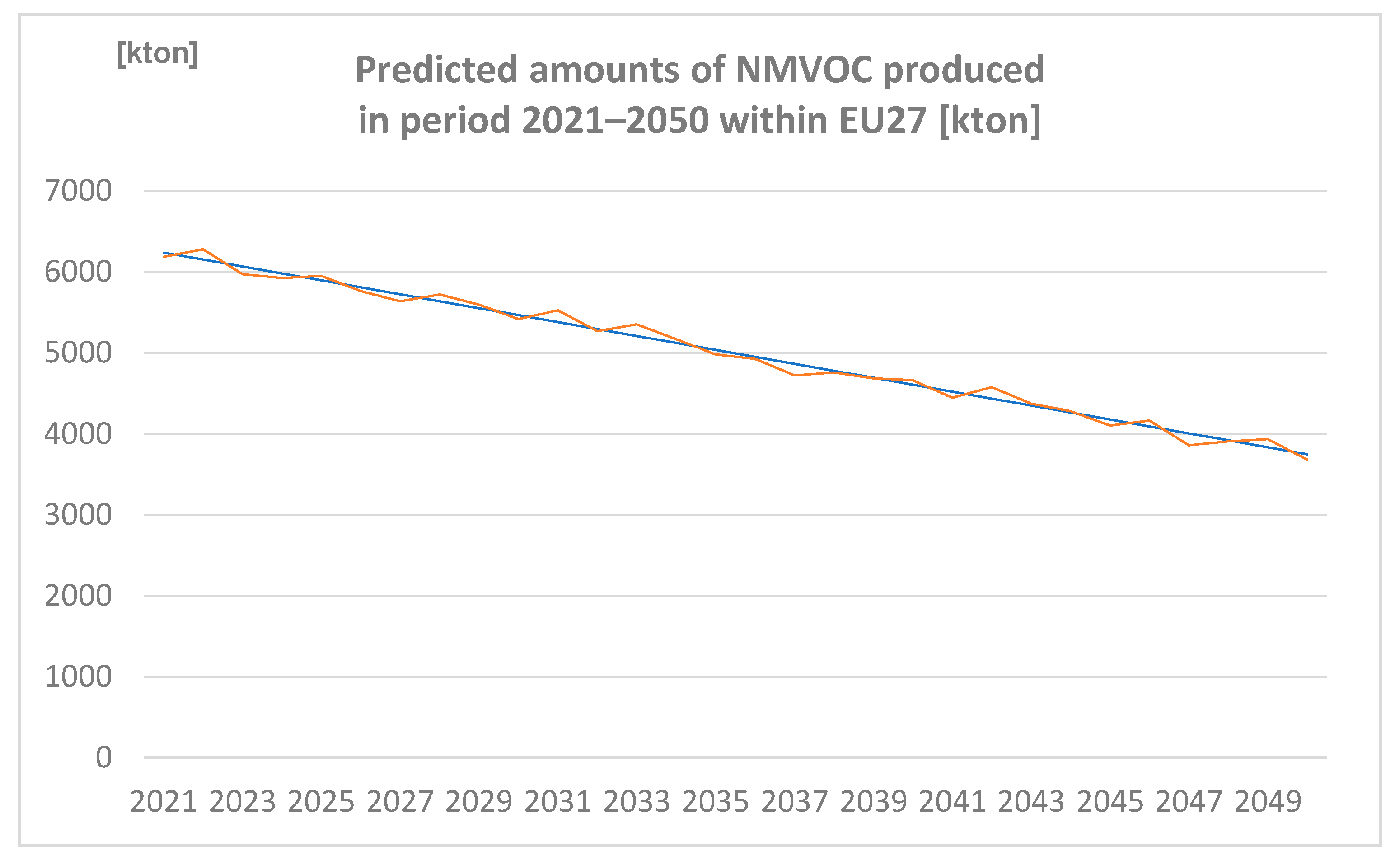
3.2.6. Amounts of NMVOC Produced in the Period 2021–2050 within EU27 [kton] Predicted by Spreadsheet and Neural Network
4. Discussion
5. Conclusions
Funding
Institutional Review Board Statement
Informed Consent Statement
Data Availability Statement
Conflicts of Interest
References
- Cristea, A.; Hummels, D.; Puzzello, L.; Avetisyan, M. Trade and the greenhouse gas emissions from international freight transport. J. Environ. Econ. Manag. 2013, 65, 153–173. [Google Scholar] [CrossRef]
- Llano, C.; Pérez-Balsalobre, S.; Pérez-García, J. Greenhouse Gas Emissions from Intra-National Freight Transport: Measurement and Scenarios for Greater Sustainability in Spain. Sustainability 2018, 10, 2467. [Google Scholar] [CrossRef]
- Antikainen, R.; Mattila, T. GHG Emissions and Fossil Fuel Dependency Scenario. In FreightVision—Scenario Building; 7th Framework Programme for Research; AustriaTech: Vienna, Austria, 2009. [Google Scholar]
- Tavasszy, L.; Piecyk, M. Sustainable Freight Transport. Sustainability 2018, 10, 3624. [Google Scholar] [CrossRef]
- Rich, J.; Brocker, J.; Hansen, C.O.; Korchenewych, A.; Nielsen, O.A.; Vuk, G. Report on Scenario, Traffic Forecast and Analysis of Traffic on the TEN-T, Taking into Consideration the External Dimension of the Union-Trans-Tools Version 2, Model and Data Improvements; DG TREN: Copenhagen, Denmark, 2009. [Google Scholar]
- Helmreich, S.; Mattila, T.; Antikainen, R.; Hansen, C.O.; Malinovský, V. Development of Strategic Scenarios of European Transportation. In Interim Report WP6.1 of FreightVision Project; AustriaTech: Vienna, Austria, 2011. [Google Scholar]
- EUROSTAT. Agriculture, Forestry and Fishery Statistics. 2016. Available online: https://ec.europa.eu/eurostat (accessed on 4 September 2022).
- Sajid, M.J.; Khan, S.A.R.; Gonzalez, E.D.R.S. Identifying contributing factors to China’s declining share of renewable energy consumption: No silver bullet to decarbonisation. Environ. Sci. Pollut. Res. 2022, 1–16. [Google Scholar] [CrossRef] [PubMed]
- Neubauer, J. Periodicita v Časové Řadě, Její Popis a Identifikace, Exponenciální Vyrovnávání (Periodicity in Time Series, its Description, and Identification, Exponential Smoothing), Study Materials; University of Defence: Brno, Czech Republic, 2020; pp. 14–16. Available online: https://k101.unob.cz/~neubauer/pdf/ekon_casove_rady_periodicita.pdf (accessed on 17 August 2021). (In Czech)
- Kačer, P. Vícevrstvá neuronová síť (Multi-Layer Neural Network). Bachelor´s Thesis, Department of Control and Instrumentation, Faculty of Electrical Engineering and Communications, Brno University of Technology, Brno, Czech Republic, 2013. (In Czech). [Google Scholar]
- Melart, S. Microsoft Office 2016: The Complete Guide; CreateSpace Publishing: Scotts Valley, CA, USA, 2015; ISBN 9781519282347. [Google Scholar]
- Dobešová, Z. ORANGE—Praktický Návod Do Cvičení Předmětu; Palacký University Olomouc: Olomouc, Czech Republic, 2022. (In Czech) [Google Scholar]
- Brandejský, T. Floating Data Window Movement Influence to Genetic Programming Algorithm Efficiency. In Computational Statistics and Mathematical Modeling Methods in Intelligent Systems, Proceedings of the 3rd Computational Methods in Systems and Software; Silhavy, P., Ed.; Springer: Cham, Switzerland, 2019; Volume 2, pp. 24–30. ISBN 978-3-030-31361-6. ISSN 2194-5357. [Google Scholar]
- Sajid, M.J. Machine Learned Artificial Neural Networks vs. Linear Regression: A Case of Chinese Carbon Emissions. In IOP Conference Series: Earth and Environmental Science, Proceedings of the 4th International Conference on Environmental and Energy Engineering, Sanya, China, 12–15 March 2020; IOP Publishing Ltd.: Bristol, UK, 2020; Volume 495. [Google Scholar] [CrossRef]
- Hallman, J. A Comparative Study on Linear Regression and Neural Networks for Estimating Order Quantities of Powder Blends. Master’s Thesis, School of Electrical Engineering and Computer Science, KTH Royal Institute of Technology, Stockholm, Sweden, 2019; pp. 49–53. Available online: http://www.diva-portal.org/smash/get/diva2:1383464/FULLTEXT01.pdf (accessed on 15 June 2022).
- Hlaváč, V. Neural Network for the identification of a functional dependence using data preselection. Neural Netw. World 2021, 31, 109–124. [Google Scholar] [CrossRef]
- Nakhaei, F.; Mosavi, M.R.; Sam, A.; Vaghei, Y. Recovery and grade accurate prediction of pilot plant flotation column concentrate: Neural network and statistical techniques. Int. J. Miner. Process. 2012, 110–111, 140–154. [Google Scholar] [CrossRef]
- Malinovský, V. Predicting Trends in Cereal Production in the Czech Republic by Means of Neural Networks. AGRIS On-Line Pap. Econ. Inform. 2021, 1, 87–103. [Google Scholar] [CrossRef]
- Svítek, M. Quantum multidimensional models of complex systems. Neural Netw. World 2019, 29, 363–371. [Google Scholar] [CrossRef]
- Malinovský, V. Comparative analysis of freight transport prognoses results provided by transport system model and neural network. Neural Netw. World 2021, 31, 239–259. [Google Scholar] [CrossRef]


| Year | Nitrogen Oxides [t] | Sulphur Oxides [t] | Ammonia [t] | Particles <2.5 μm [t]< | Particles <10 μm [t]< | Non-Methane Volatile Organic Compounds [t] |
|---|---|---|---|---|---|---|
| 1990 | 14,901,060 | 21,027,390 | 4,916,130 | 2,853,320 | 4,268,570 | 15,869,850 |
| 1991 | 14,661,480 | 18,962,410 | 4,668,480 | 2,770,890 | 4,117,520 | 15,203,760 |
| 1992 | 14,330,450 | 16,986,670 | 4,424,300 | 2,600,970 | 3,848,030 | 14,611,660 |
| 1993 | 13,732,310 | 16,290,640 | 4,290,110 | 2,545,090 | 3,743,440 | 14,044,140 |
| 1994 | 13,271,010 | 15,257,280 | 4,174,810 | 2,394,950 | 3,535,540 | 13,053,260 |
| 1995 | 12,956,820 | 13,904,350 | 4,107,060 | 2,319,530 | 3,391,500 | 12,702,510 |
| 1996 | 12,819,520 | 13,087,430 | 4,146,200 | 2,341,570 | 3,398,750 | 12,516,040 |
| 1997 | 12,384,550 | 12,095,900 | 4,113,820 | 2,233,740 | 3,253,500 | 12,086,710 |
| 1998 | 12,092,420 | 10,903,730 | 4,122,610 | 2,132,070 | 3,170,040 | 11,730,360 |
| 1999 | 11,747,860 | 9,708,620 | 4,099,850 | 2,033,370 | 3,004,410 | 11,205,560 |
| 2000 | 11,391,420 | 8,685,400 | 4,031,680 | 1,935,520 | 2,892,440 | 10,598,430 |
| 2001 | 11,241,240 | 8,335,780 | 4,000,790 | 1,884,810 | 2,854,730 | 10,177,200 |
| 2002 | 11,044,840 | 7,951,150 | 3,938,270 | 1,771,000 | 2,725,410 | 9,772,590 |
| 2003 | 10,943,580 | 7,551,640 | 3,912,460 | 1,817,580 | 2,774,510 | 9,535,470 |
| 2004 | 10,816,840 | 7,189,600 | 3,872,030 | 1,763,000 | 2,725,130 | 9,258,790 |
| 2005 | 10,649,440 | 6,880,950 | 3,824,300 | 1,747,110 | 2,683,650 | 9,080,750 |
| 2006 | 10,396,420 | 6,670,110 | 3,798,120 | 1,705,760 | 2,643,890 | 8,887,150 |
| 2007 | 10,102,010 | 6,342,450 | 3,822,240 | 1,682,400 | 2,596,010 | 8,542,590 |
| 2008 | 9,404,150 | 4,809,430 | 3,725,190 | 1,660,070 | 2,555,080 | 8,234,930 |
| 2009 | 8,701,210 | 4,006,880 | 3,646,960 | 1,588,700 | 2,418,430 | 7,696,650 |
| 2010 | 8,500,370 | 3,685,760 | 3,614,760 | 1,610,500 | 2,423,640 | 7,648,970 |
| 2011 | 8,189,730 | 3,581,300 | 3,584,500 | 1,492,090 | 2,289,350 | 7,262,400 |
| 2012 | 7,869,350 | 3,158,480 | 3,571,470 | 1,495,340 | 2,248,970 | 7,095,560 |
| 2013 | 7,514,780 | 2,734,880 | 3,571,760 | 1,470,990 | 2,219,370 | 6,874,490 |
| 2014 | 7,253,620 | 2,540,260 | 3,594,520 | 1,345,810 | 2,081,390 | 6,649,600 |
| 2015 | 7,113,550 | 2,440,410 | 3,635,460 | 1,356,510 | 2,092,960 | 6,615,750 |
| 2016 | 6,899,690 | 2,068,400 | 3,633,290 | 1,332,910 | 2,060,410 | 6,571,950 |
| 2017 | 6,751,610 | 2,029,410 | 3,647,290 | 1,333,590 | 2,067,410 | 6,634,580 |
| 2018 | 6,475,440 | 1,884,460 | 3,613,460 | 1,290,730 | 2,026,410 | 6,498,640 |
| 2019 | 6,140,700 | 1,649,110 | 3,532,320 | 1,251,260 | 1,978,830 | 6,408,660 |
| 2020 | 6,004,312 | 1,522,897 | 3,482,297 | 1,248,788 | 1,968,812 | 6,324,478 |
| Year | Nitrogen Oxides [t] | Sulphur Oxides [t] | Ammonia [t] | Particulates <2.5 μm [t]< | Particulates <10 μm [t]< | Non Methane Volatile Organic Compounds [t] |
|---|---|---|---|---|---|---|
| 2021 | 5,820,648 | 1,366,942 | 3,447,222 | 1,212,296 | 1,936,785 | 6,238,565 |
| 2022 | 5,656,243 | 1,219,708 | 3,412,147 | 1,175,878 | 1,904,817 | 6,152,666 |
| 2023 | 5,491,839 | 1,072,475 | 3,377,072 | 1,139,461 | 1,872,849 | 6,066,767 |
| 2024 | 5,327,434 | 925,241 | 3,341,996 | 1,103,044 | 1,840,881 | 5,980,868 |
| 2025 | 5,163,029 | 778,008 | 3,306,921 | 1,066,627 | 1,808,913 | 5,894,969 |
| 2026 | 4,998,624 | 630,774 | 3,271,846 | 1,030,210 | 1,776,945 | 5,809,070 |
| 2027 | 4,834,220 | 483,541 | 3,236,771 | 993,793 | 1,744,977 | 5,723,171 |
| 2028 | 4,669,815 | 336,307 | 3,201,696 | 957,376 | 1,713,009 | 5,637,272 |
| 2029 | 4,505,410 | 189,074 | 3,166,621 | 920,959 | 1,681,040 | 5,551,373 |
| 2030 | 4,341,005 | 41,840 | 3,131,545 | 884,542 | 1,649,072 | 5,465,474 |
| 2031 | 4,176,601 | 0 | 3,096,470 | 848,125 | 1,617,104 | 5,379,574 |
| 2032 | 4,012,196 | 0 | 3,061,395 | 811,708 | 1,585,136 | 5,293,675 |
| 2033 | 3,847,791 | 0 | 3,026,320 | 775,291 | 1,553,168 | 5,207,776 |
| 2034 | 3,683,386 | 0 | 2,991,245 | 738,874 | 1,521,200 | 5,121,877 |
| 2035 | 3,518,981 | 0 | 2,956,170 | 702,457 | 1,489,232 | 5,035,978 |
| 2036 | 3,354,577 | 0 | 2,921,094 | 666,039 | 1,457,264 | 4,950,079 |
| 2037 | 3,190,172 | 0 | 2,886,019 | 629,622 | 1,425,295 | 4,864,180 |
| 2038 | 3,025,767 | 0 | 2,850,944 | 593,205 | 1,393,327 | 4,778,281 |
| 2039 | 2,861,362 | 0 | 2,815,869 | 556,788 | 1,361,359 | 4,692,382 |
| 2040 | 2,696,958 | 0 | 2,780,794 | 520,371 | 1,329,391 | 4,606,483 |
| 2041 | 2,532,553 | 0 | 2,745,719 | 483,954 | 1,297,423 | 4,520,584 |
| 2042 | 2,368,148 | 0 | 2,710,643 | 447,537 | 1,265,455 | 4,434,685 |
| 2043 | 2,203,743 | 0 | 2,675,568 | 411,120 | 1,233,487 | 4,348,786 |
| 2044 | 2,039,339 | 0 | 2,640,493 | 374,703 | 1,201,519 | 4,262,886 |
| 2045 | 1,874,934 | 0 | 2,605,418 | 338,286 | 1,169,550 | 4,176,987 |
| 2046 | 1,710,529 | 0 | 2,570,343 | 301,869 | 1,137,582 | 4,091,088 |
| 2047 | 1,546,124 | 0 | 2,535,268 | 265,452 | 1,105,614 | 4,005,189 |
| 2048 | 1,381,720 | 0 | 2,500,192 | 229,035 | 1,073,646 | 3,919,290 |
| 2049 | 1,217,315 | 0 | 2,465,117 | 192,618 | 1,041,678 | 3,833,391 |
| 2050 | 1,052,910 | 0 | 2,430,042 | 156,200 | 1,009,710 | 3,747,492 |
| Year | Nitrogen Oxides [t] | Sulphur Oxides [t] | Ammonia [t] | Particulates <2.5 μm [t]< | Particulates <10 μm [t]< | Non Methane Volatile Organic Compounds [t] |
|---|---|---|---|---|---|---|
| 2021 | 5,954,769 | 1,341,112 | 3,306,595 | 1,259,483 | 2,038,350 | 6,187,751 |
| 2022 | 5,511,324 | 1,346,740 | 3,326,178 | 1,270,856 | 1,802,179 | 6,281,076 |
| 2023 | 5,450,415 | 1,068,363 | 3,234,359 | 1,240,298 | 1,767,269 | 5,970,638 |
| 2024 | 5,421,707 | 1,046,687 | 3,334,266 | 1,130,779 | 1,852,372 | 5,923,834 |
| 2025 | 5,108,164 | 764,739 | 3,380,054 | 1,107,260 | 1,683,486 | 5,948,722 |
| 2026 | 4,913,650 | 750,567 | 3,181,173 | 1,037,507 | 1,680,868 | 5,761,074 |
| 2027 | 4,863,381 | 403,889 | 3,315,392 | 940,454 | 1,702,234 | 5,637,475 |
| 2028 | 4,637,419 | 242,763 | 3,139,806 | 966,059 | 1,584,052 | 5,719,721 |
| 2029 | 4,489,271 | 302,982 | 3,138,580 | 1,066,913 | 1,640,162 | 5,594,310 |
| 2030 | 4,347,231 | 116,087 | 3,125,490 | 867,227 | 1,781,899 | 5,415,198 |
| 2031 | 4,050,147 | −66,349 | 3,161,219 | 816,074 | 1,628,682 | 5,524,755 |
| 2032 | 3,899,745 | 22,860 | 3,173,472 | 912,925 | 1,474,016 | 5,269,354 |
| 2033 | 3,738,309 | 0 | 2,900,424 | 853,859 | 1,559,637 | 5,352,088 |
| 2034 | 3,722,490 | 0 | 2,848,026 | 705,654 | 1,401,767 | 5,166,573 |
| 2035 | 3,506,624 | 0 | 2,997,306 | 772,890 | 1,624,687 | 4,979,976 |
| 2036 | 3,210,652 | 0 | 2,826,739 | 595,473 | 1,447,588 | 4,925,885 |
| 2037 | 3,141,298 | 0 | 2,794,423 | 707,142 | 1,450,066 | 4,722,056 |
| 2038 | 3,077,768 | 0 | 2,805,856 | 723,679 | 1,512,396 | 4,757,959 |
| 2039 | 2,788,151 | 0 | 2,962,224 | 621,784 | 1,394,534 | 4,685,620 |
| 2040 | 2,602,086 | 0 | 2,759,143 | 560,146 | 1,470,097 | 4,661,514 |
| 2041 | 2,670,503 | 0 | 2,609,174 | 624,495 | 1,313,167 | 4,444,152 |
| 2042 | 2,446,321 | 0 | 2,731,840 | 501,841 | 1,353,022 | 4,575,003 |
| 2043 | 2,119,749 | 0 | 2,542,882 | 321,021 | 1,147,957 | 4,371,095 |
| 2044 | 1,958,518 | 0 | 2,603,874 | 437,067 | 1,099,716 | 4,279,230 |
| 2045 | 1,797,420 | 0 | 2,594,455 | 313,197 | 1,047,350 | 4,101,911 |
| 2046 | 1,704,763 | 0 | 2,568,640 | 294,273 | 1,252,113 | 4,163,454 |
| 2047 | 1,418,529 | 0 | 2,564,543 | 199,272 | 1,023,958 | 3,859,325 |
| 2048 | 1,467,217 | 0 | 2,589,877 | 284,154 | 1,091,714 | 3,907,173 |
| 2049 | 1,190,768 | 0 | 2,403,692 | 170,732 | 980,604 | 3,932,860 |
| 2050 | 1,178,674 | 0 | 2,477,832 | 230,263 | 876,873 | 3,681,273 |
Publisher’s Note: MDPI stays neutral with regard to jurisdictional claims in published maps and institutional affiliations. |
© 2022 by the author. Licensee MDPI, Basel, Switzerland. This article is an open access article distributed under the terms and conditions of the Creative Commons Attribution (CC BY) license (https://creativecommons.org/licenses/by/4.0/).
Share and Cite
Malinovsky, V. Neural Networks as an Alternative Tool for Predicting Fossil Fuel Dependency and GHG Production in Transport. Sustainability 2022, 14, 11231. https://doi.org/10.3390/su141811231
Malinovsky V. Neural Networks as an Alternative Tool for Predicting Fossil Fuel Dependency and GHG Production in Transport. Sustainability. 2022; 14(18):11231. https://doi.org/10.3390/su141811231
Chicago/Turabian StyleMalinovsky, Vit. 2022. "Neural Networks as an Alternative Tool for Predicting Fossil Fuel Dependency and GHG Production in Transport" Sustainability 14, no. 18: 11231. https://doi.org/10.3390/su141811231
APA StyleMalinovsky, V. (2022). Neural Networks as an Alternative Tool for Predicting Fossil Fuel Dependency and GHG Production in Transport. Sustainability, 14(18), 11231. https://doi.org/10.3390/su141811231