Abstract
With the development of intelligent transportation systems, research into intelligent traffic signal control has received considerable attention. To date, many traffic signal control models have been studied, where most of the models concentrate on how to minimize travel time, vehicle delay, and the number of stops or how to maximize capacity. This study introduces the Garra Rufa–inspired (GRI) algorithm, which is used to optimize traffic signal control modelling considering the number of vehicles in a queue. GRI has the characteristics of using the decision variables of the code as the operation object, directly using the objective function value for the search information, using multiple search points at the same time, and using probability search technology. Theoretical analysis of intelligent optimization and research into application methods were carried out to resolve the problem of traffic signal optimization control. The output of the GRI algorithm was compared, calibrated, and validated with SIDRA. Furthermore, to obtain more comprehensive results, the genetic algorithm (GA) and particle swarm optimization (PSO) were also compared. The results of the analysis show that the GRI decreases by 10.1% (intersection A) and 16.5% (intersection B) in the number of vehicles in the queue.
1. Introduction
With the acceleration of urbanization, the conflict between the supply and demand of road traffic is increasing rapidly, and traffic congestion has become a major problem affecting urban development [1]. Traffic signal control systems are trying to solve urban traffic congestion effectively [2]. The intersections are the most important part of the entire traffic system [1,2]. Due to the rapid increase in the number of motor vehicles, the lagging construction of transportation facilities, and inadequate management measures, traffic jams at intersections are becoming more and more problematic, affecting the capacity of the urban road network [3,4]. The vehicles repeatedly diverge, merge, and cross at intersections, making traffic conditions complex, so intersections have become bottlenecks, restricting urban road traffic functions [4]. To maintain the normal operation of urban traffic, it is necessary to strengthen traffic control and management, actively carry out research on intersections, and strive to improve the traffic capacity of intersections. Due to the large traffic flow at urban road intersections, signal control is usually adopted [5]. The control of traffic signal timing optimization at intersections can alleviate increasingly tight urban traffic congestion and improve the efficiency of urban traffic operations.
Since the introduction of signalized intersections, schemes such as phase design and calculation of cycle length and phase durations to improve intersection capacity have been studied [4]. Traffic congestion has created unnecessary time consumption and pollutant emissions by using fossil fuels, which has become a serious social problem [5]. Considering the poor transport infrastructure, scholars and transport practitioners have mainly focused on the supply and development of physical transport facilities [6]. However, supplying new facilities, especially road expansion, may minimize congestion temporarily, and they will attract more future automobile demand, which is called induced demand, causing congestion [6,7]. In many cases, the option of supplying new road facilities is no longer considered a feasible solution for the longer term. Thus, traffic management strategies, such as signal timing optimization, have been suggested as suitable solutions [7].
Webster first tried to provide signal timing based on minimum average delay in 1958 [8]. Since then, several studies have attempted to solve or reduce congestion problems at intersections by providing the best cycle length (the total signal time needed to serve all signal phases, including the green time), plus any change interval and phase duration (any traffic signal display that has a unique set of timings for directing the movement of a single vehicle or pedestrian) [9,10,11]. Another researcher, Akçelik, provided optimal signal timing with the parking compensation coefficient, which is related to the number of stops and vehicle delay time [9]. Moreover, bilevel programming-based research was conducted [10,11,12], and each level considered traffic signal, stochastic user equilibrium, total travel time, capacity, and vehicle emission [11]. In addition, other concepts, such as the cell transmission model and lane change models, have been applied to find the optimal signal timing for enhancing intersection capacity [13,14].
At the same time, many scholars have shifted their perspective to computational intelligence-based models, such as fuzzy models, genetic algorithms (GA), swarm intelligence, and so on, to relieve congestions at intersections [15]. These methods typically minimize objectives (e.g., vehicle delay, stop, queue, based on calculated signal timing) [16]. A study by Niittymäki and Pursula [15] used the average delay of vehicles as the performance criteria for the intersection and proposed a new fuzzy control algorithm to optimize the timing of the intersection. GA was introduced into the fuzzy control of urban intersection signals to optimize the parameters of the fuzzy controller globally [16,17]. In [18], a hybrid method (fuzzy neural network) was suggested to reduce delay time on each approach at the intersections. The fuzzy control method was also proposed for intersection control based on a double-loop phase structure [17]. Heuristic methods, such as fuzzy control, do produce a better solution, but lack a certain mathematical rigor and cannot guarantee that the obtained solution is the optimal solution [19].
Currently, typical intelligent algorithms, namely, GA and particle swarm optimization (PSO), are widely used to optimize traffic flows at intersections [20]. In [21], GA was applied for traffic signal timing optimization based on drivers’ routing concepts and can increase traffic flow at intersections and save time when compared with typical heuristic algorithms. Other studies by Turky et al. and Odeh also attempted to apply GA to reduce vehicle and pedestrian queues and save time at intersections [22,23]. In [24], multiobjectives (vehicle delay and intersection capacity) were optimized by GA based on the Hu Cheng Hunan Road intersection in Shanghai. The author concluded that the proposed GA can provide 4 s of delay reduction and 29 passenger car unit per hour (pcu/h) intersection enhancement. Moreover, a comparison study was conducted by Possel et al. and in their study, simulated annealing was compared with GA [25]. In [26], the optimum cycle length and phase durations were optimized for traffic networks based on the areawide optimization method. The microscopic simulation software Paramics was utilized for model validation, and the results showed that 23.7% of travel time can be reduced.
Concerning PSO, many studies regarding traffic flow optimization were performed as well. In [27], the optimal cycle length and green time were calculated by PSO and compared with a fully actuated control algorithm. In [28], PSO was applied for optimizing traffic signal cycles using the SUMO traffic simulation tool, and the modified PSO with AIMSUN software was applied by Wijaya et al. based on the road network in Japan [29]. Another study by Jia et al. regarded the total number of vehicles at the intersection as the objective function and used the PSO algorithm to solve the timing plan [30]. In [31,32], PSO was tested and implemented to provide the optimal cycle length and phase durations to reduce average delay time and the number of stops and increase intersection capacity. Furthermore, other studies tried to optimize intersections and networks via adjustment of signal timing plans using various swarm intelligent search algorithms [32,33].
A traffic signal timing plan is complicated, and the GA and parallel algorithms only use one kind of computational algorithm to find the optimal cycle length for enhancing intersection capacity [34]. Although a GA can reach a solution easily and the PSO can converge faster, they both have a drawback in that it is easy to fall into local optimization [35]. In addition, the majority of intersection optimization studies tend to focus on theoretical algorithm development based on normal four signal phases, and select average vehicle delay, the number of stops, and capacity as objectives [36]. Additionally, most studies relating to signal timing optimization tend to analyze intersection capacity by relying on microscopic simulation, namely, VISSIM, AIMSUN, and SUMO.
This paper, therefore, introduces a Garra Rufa–inspired (GRI) algorithm for solving function optimization problems and proposed to improve the traffic signal control strategy at an intersection to reduce the number of vehicles in the queue as the main objective. The proposed GRI model optimized the number of vehicles in the queue on each approach and was tested on two intersections in Jungbu-daero, Yongin City, Korea. Furthermore, to obtain more comprehensive results, the GRI was compared with typical GA and PSO, and then the optimized signal timing was applied to SIDRA to obtain the various outputs, including capacity, travel speed, delays, and CO2 emission. The analytical model SIDRA is user-friendly for modelling, calibration, and validation [37], and it includes the US Highway Capacity Manual method [38] and produces acceptable and rich outputs, especially in delay time estimation, for signalized intersections [39].
2. Background
2.1. Genetic Algorithm and Particle Swarm Optimization
The GA and PSO can be widely used to investigate optimal signal timing. The nonlinear model of signal timing optimization as established has the characteristics of irregularity and discontinuity. The fitness function defined by the genetic algorithm has strong adaptability. It can be found even in the case of irregularity, discontinuity, or noise; therefore, GA and PSO are suitable for solving the signal timing optimization model.
The basic fundamental of GA as the first global adaptive probabilistic search algorithm is based on the principles of natural selection and genetics and guided by the natural selection mechanism of survival of the fittest in biological evolution and the genetic mechanism of reproduction and evolution in the biological world.
The specific steps of the GA are as follows:
(1) Setting of initial parameters: Population size (n), crossover probability (), mutation probability (), evolutionary algebra .
(2) Chromosome coding: Selects the floating-point coding method, which can overcome a series of problems of binary codings, such as long coding string, sharp expansion of search space, and a large amount of computation due to the precision requirement of the optimization problem. Among them, the coding length of the individual is equal to the number of bits of its decision variable.
(3) Fitness function: The effective green light time of each phase is used as the optimization variable, and the average delay is used as the optimization objective function to solve the minimum value of the average delay of the plane intersection. To meet the conditions of the fitness function, the corresponding relationship between the fitness function () and the objective function () needs to be established. The inverse of the objective function is used as the fitness function, namely,
(4) The roulette method is chosen as the selection operator, which is a random selection strategy with the refund. Each individual in the group is a part of the sector in the disc. The larger the area of the sector, the higher the fitness value of the individual, and the greater the probability of the individual entering the next round of selection. Assuming that the number of individuals in the population is (), and the fitness of individual is (), then its probability of being selected is:
(5) Choose the real number crossover method [19], which refers to the generation of two new individuals by the linear combination of two gene individuals. For example, the crossover operation method () of the n-th chromosome (, ) at the position is:
where is a random number in the interval [0, 1].
(6) Variation: Nonuniform variation is used. The method of mutating a gene of the -th individual is as follows:
where is the upper bound of the gene, is the lower bound of the gene, is the random number, , and is the current iteration number [0, 1].
(7) Evolution termination conditions: The maximum evolutionary algebra is set as T. When the number of iterations satisfies the condition , the optimal solution based on the GA is the individual with the highest fitness value in the population, and finally, the individual decoding work is performed to obtain the signal timing optimization scheme of the plane intersection [20].
The basic principle of the PSO algorithm is a global random search algorithm based on swarm intelligence proposed by simulating the foraging process of birds to initialize a group of particles in the solution space [14]. The characteristics of each particle are represented by three indicators: position, speed, and fitness that the position of each particle represents a potential optimal solution, and the position of the food represents the global optimal solution. Each particle approaches the position of the optimal solution by continuously adjusting the direction, speed, and fitness function. As the PSO has the advantages of easy implementation, high precision, and fast convergence, the operation rules are simpler than the GA, and it has certain advantages in solving practical problems. This paper adopts the PSO algorithm.
The main iterative steps of the algorithm are as follows:
(1) Set the initial current number of iterations, where . The particle number size is 10, and set the solution space. The number of variables is 1, and generate the initial position matrix and initial velocity matrix of the particle swarm .
(2) Initialize the individual historical optimal value and the global optimal value of the population , and initialize the individual historical optimal position vector and the global optimal position vectors.
(3) Calculate the fitness value of each particle ; compare the fitness value of each particle with the individual historical optimal value . If it is better than , then let , and let the current position of the particle be its historical optimal position = ; otherwise, do not change and .
(4) Compare the individual historical optimal value and in turn the population optimal value of each particle . If the current value for is better than the current value , let the historical optimal position of the particle be the global historical optimal position of the population ; otherwise, the sum will not be changed.
(5) The number of iterations is incremented by 1, and the velocity and position of each particle are updated:
where is the velocity vector of the particle when the number of iterations is t, is the position vector of the particle when the number of iterations is t, is the individual historical optimal value of the particle when the number of iterations is t, and is the global history of the particle when the number of iterations is the optimal value. To adjust the parameters , these parameters are set as 0.9, 1, and 1, respectively.
(6) If the algorithm satisfies the convergence criterion or reaches the maximum number of iterations , execute step (6); otherwise, execute step (3).
(7) The algorithm ends, and the global optimal position of the population is and the global historical optimal value is output .
2.2. Garra Rufa–Inspired (GRI) Algorithm
The GRI algorithm is an adaptive global optimization probability search algorithm formed by simulating the genetic and evolutionary processes in the natural biological environment. It is one of a class of robust search algorithms that can be used for the optimization calculation of complex systems. It has the characteristics of using the decision variables of the code as the operation object, directly using the objective function value for the search information, using multiple search points at the same time, and using probability search technology [35].
Depending on the difference in the work, the process of the GRI approach is presented in the following steps. The main process can be divided into three steps:
Step (1) Initial stage of the search
In the initial stage of the fish colony search, the fishes can only move a short distance in one direction and update the pheromones of that direction, and the fishes routing strategy is to select the route with the greatest probability of finding the most pheromones. It is easier to concentrate on a few shorter distances, resulting in the search outcome being a local optimum rather than a global optimum. In this initial stage, the accumulation factor and the volatilization factor are set as:
where represents the pheromone accumulated by the fish group at the i-th step on the move toward , and represents the pheromones released by the fish group at the i-th step to search for other fish. Since the work of the reconnaissance fish group and that of the search fish group are different, the pheromone increment will be adjusted according to different fish groups:
where represents the pheromone increment function of the direction j selected by the fishes in the fish group k at the i-th step. To improve the ability of fishes to find a better direction and speed up the algorithm to search for the full optimal solution, is introduced in represents the search process local minimum and local maximum. It compares the local optimal value with the current objective function value. Meanwhile, a positive constant is introduced to balance the variation range of .
Step (2) Search intermediate stage
In the middle stage of the GRI search, fishes need to accumulate and develop continuously. For the first half of the search at this stage, the development ability of the fishes should be improved so that the fishes can search for different directions and enrich the diversity of the candidate selections. To meet the different performance requirements of focusing on the accumulation in the early stage of the search stage and focusing on development in the later stage:
where represents the probability that the fishes in the fish group choose direction j at the i-th step, represents all the directions that the fishes can choose at the i-th step, represents the fishes in the fish group choosing the attraction of direction j at the step, and , are random numbers of [0, 1]. In this search stage, the pheromone is updated according to Equations (11) and (12):
where ρ represents the volatilization factor of the pheromone in the selected direction, ρ’ represents the volatilization factor of the pheromone in the unselected direction, and represents the accumulation factor of the direction taken by the m-th fish in the fish group k. Since the direction-finding process of fishes is similar to the learning process of humans, the forgetting curve in the learning process can be compared with the pheromone volatilization factor ρ in Equation (11). The variable range is set, and the acceleration factor decreases as the number of iterations increases. When is large, it can improve the ability of fishes to find a new direction. When ρ is small, it can improve the ability of fishes to select the optimal direction. When is related to the value of the objective function, the better the target value corresponding to the direction sought, and the larger the value. The calculation method of is as follows:
where represents the number of fishes in each group , and ) represents the position of the objective function value of the direction sought by the m-th fish in the fish group in this iteration.
Step (3) Exchange search late stage
To improve the ability to search for the optimal solution, a new group of fishes is added to the search at this stage, responsible for the local search to find a better solution around the direction with the most pheromones. The new fish group will maintain a new local pheromone matrix, taking the part of Equation (6) and the pheromone update Equation (10) as the transfer rule and setting the iteration threshold, marking the local search Start. Since this group of fishes is mainly used for development, the value of Equation (10) is small, and the and values do not change with the number of iterations.
3. Research Methodology
3.1. Research Flow
This study is composed of six steps as outlined in Figure 1. In the GRI algorithm, signal timing schemes and optimization methods are investigated and compared with other methods. The GRI algorithm is capable of considering the number of vehicles in a queue proposed. The third step consists of study area selection and intersection data collection in Yongin City, South Korea. Moreover, collected data, including traffic volume, the number of vehicles in a queue on each approach, cycle length, and phase durations, are utilized in SIDRA model calibration and validation based on RMSE and GEH statistic tests. In the next step, the optimized signal timing is applied to the SIDRA 9 software (SIDRA solution, Greythorn, VIC, Australia), where rich information is obtained. In the final step, a comparison study is presented with capacity, travel speed, delays, and CO2 output using the SIDRA platform. In addition, typical GA and PSO are also compared with the GRI algorithm.
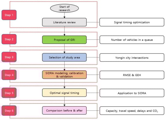
Figure 1.
Research flowchart.
3.2. RMSE and GEH
This study applied popular statistical procedures, including root mean square error (RMSE) and Geoff E. Havers (GEH), in order to verify the fitness of the proposed model. RMSE is widely employed for model evaluation as a standard method [40]. RMSE describes the sample standard deviation through a relationship between the outputs of two groups as expressed in Equation (14). The smaller value of RMSE indicates better model agreement [41,42]:
where n is the number of periods, is the model outputs, is the observation, and is the mean of observations.
The GEH statistic is a type of the chi-squared statistic, and this method can be used to compare model outputs and field data [43,44], and it is widely used in traffic engineering and modelling [45]. The goodness of fit can be judged by the calculated value and the value of GEH, which is less than five, and the model output fits with the observed data properly [46]. The relationship between two outputs can be expressed in Equation (15):
where is the estimated output by the model, and is the observation.
3.3. Proposed Model
In this paper, a passenger car is considered “vehicle”. The GRI algorithm is used to optimize the timing of signals, and it is performed according to the signal cycle changes. For the intersection controlled by the phase signal, the release status of the vehicle in different phases and different lanes can be represented by a coefficient matrix , that is,
where i is the phase number, and the values 1, 2, 3, and 4 are the corresponding phases; j is the direction number; the values 1, 2, 3, and 4 are the four approaches at the intersection direction, k is the lane number; and the values 1, 2, and 3 are the left, straight, and right turn lanes at each approach of the intersection, respectively. An example of four-phase signal control (lag dual left) is as follows:
Take the intersection capacity as the optimization objective function, minimizing the number of vehicles at the intersection, thereby maximizing the vehicle capacity. If ti (i = 1, 2, 3, 4) is the timing of each phase of the intersection, is the vehicle arrival rate of the i-th phase, the j-th direction, and the k-th lane. Vehicles arrive in phase i, direction j, and lane k in a cycle:
If the departure rate of the passing vehicle in the i-th phase, the j-th direction, and the k-th lane during the green signal time is rijk, then the vehicles that may leave the i-th phase, the j-th direction, and the k-th lane in a cycle are:
If the number of vehicles staying in the l-th period, i-th phase, j-th direction, and k-th lane, then it can be written as:
where i is 1, 2, 3, 4; j is 1, 2, 3, 4; and k is 1, 2, 3. When i is 1, is the vehicle staying in the l- cycle, the j-th direction, the k-th lane, and the fourth phase. Therefore, the total number of vehicles (s) in the queue at the intersection at the end of the l cycle is:
According to the analysis, to maximize the traffic flow at the intersection, the number of vehicles in the queue at the intersection should be the smallest (.
Then,
The optimization is performed for the duration of each phase of the intersection as:
where T is the cycle length of the intersection signal control (sec.).
Assuming that the traffic signal timing is constant, and if the condition of Equation (23) is satisfied, find the minimum value of Equation (22). Considering the needs of pedestrian crossings, the minimum green light time for each phase should satisfy a certain domain value E (usually E ≥ 6 s); then the timing of each phase must satisfy:
where n is the number of phases in one cycle of the signal timing scheme. Therefore, for intersections controlled by four-phase signals, the timing of each phase must satisfy:
The optimal phase timing control requires the prediction of traffic flow because the arrival of vehicles is random and the change of traffic flow during a day is different with different periods. While performing signal control in the current cycle, it is necessary to predict the arriving volume in the next cycle and provide data for timing optimization in the next cycle. Optimized phase timing is to use the traffic flow information of this cycle and the previous cycle and consider the number of vehicles staying at the intersection at the current cycle. After optimization processing, the optimal timing is provided for the phase of the next cycle at the intersection. The traffic volume arriving at a single intersection in each direction can be calculated according to Equation (26):
where I is a positive integer, is the number of vehicles arriving in the first period, α is the correction coefficient (0 < α < 1), and the α absolute value is proportional to . Select the timing of each phase at the intersection as a variable, considering the practical constraints to convert the minimum value of Equation (27):
The main intersection signal timing process can be divided into five steps:
Step (1) In the initial stage of the fish colony search using Equations (6) and (7), the fish colony will evaluate the objective function Equation (27).
Step (2) Select the direction with more pheromones with a greater probability.
Step (3) Update the pheromone of the direction and the fish’s routing strategy using Equations (11) and (12). Then the fish colony will re-evaluate the objective function Equation (27).
Step (4) Responsible for the local search and trying to find the best solution around the direction with the largest number of pheromones.
Step (5) Checking the termination conditions. If met, then continue the process; otherwise, return to step 3.
4. Data Collection
An experimental analysis was conducted utilizing the flow data collected by the remote traffic microwave detectors on Yongin City roads in Korea, as recorded by the central traffic unit. Jungbu-daero in Yongin City, Korea, was selected as the research object, and the experiment comprehensively selected two intersections on Jungbu-daero in Yongin City, as depicted in Figure 2. The experiment utilized a 5 min time period to learn, train, and predict the traffic flow data to verify the effectiveness of the proposed model. The traffic volume data were obtained during peak hours from 7:30 a.m. to 8:30 a.m. on 15 April 2018.
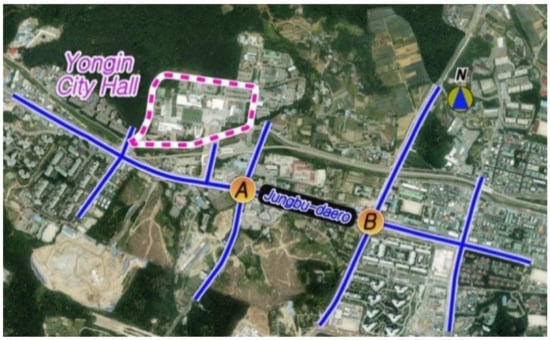
Figure 2.
Two selected intersections (A and B) on Jungbu-daero.
For the proposed model validation, a comparative study between the output from the model and SIDRA was performed. Figure 3 presents the intersection modelling in SIDRA reflecting the number of lanes, geometry features, traffic volumes, signal timing, and speed (60 km/h).
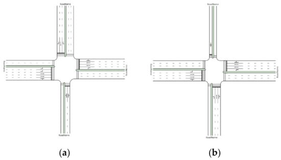
Figure 3.
Intersection modelling using SIDRA. (a) Intersection A; (b) Intersection B.
Table 1 summarizes the signal phases used for the real-time optimized control strategy for single intersection signals. Both intersections are operated with four phases; however, phases 3 and 4 are used for different directional traffic. Moreover, the two intersections have different cycle lengths (i.e., 140 s—A intersection, 120 s—B intersection).

Table 1.
Signal phase diagram of Jungbu-daero in Yongin City.
Table 2 shows the 1-h directional traffic volume at each intersection and a total of 5533 vehicles (A) and 4467 vehicles (B) that passed through each intersection during the 1-h peak. The traffic volume from the eastern to the western approach is approximately 2000 vph in both intersections, and the traffic volume from the west to the east approach is slightly less. In addition, the two intersections are composed of 3.5% of heavy vehicles, and it is converted to pcu for further analysis.
Table 2.
Peak hour directional traffic volume at each intersection.
After each modelling, the intersections were connected using the network function in SIDRA, which can evaluate two or more intersections at the same time [33]. To reflect real-life traffic conditions, signal phase sequences (Table 1), cycle length, traffic volume (Table 2), number of lanes (Figure 3), and distance between intersections (360 m) were applied.
Table 3 presents the average number of vehicles in the queue at each intersection over an hour. There are more than 30 vehicles in the queue on the eastern and the western approaches at intersection A. Moreover, intersection B has a long queue; 49.3 vehicles queued, waiting for the next cycle on the eastern approach, and 40.1 vehicles on average were observed to be waiting.
Table 3.
Number of vehicles in the queue in each approach on Jungbu-daero.
5. Results
5.1. Optimized Signal Timing and Number of Vehicles in a Queue
To establish the validity of the model, an analysis of the number of vehicles in the queue was conducted, and the results were compared with the traffic predictions under the traffic control strategy optimized by the GRI algorithm. The GRI algorithm optimized operating parameters of single intersection signal timing: population size N = 100, chromosome length n = 24, termination algebra G = 100, crossover probability Pc = 0.8, and mutation probability Pm = 0.001. The GRI algorithm was used for simulation and run for 50 cycles. Under the conditions of permitted traffic in each lane of the four directions of the intersection, if the number of vehicles released was 3600 per hour, the timing signal cycle was 160 s.
Figure 4 graphically depicts the performances of GA, PSO, and GRI following 100 iterations. The Y axis indicates an average of the number of vehicles in 1 h for all approaches, and the X axis indicates the iteration number. The GRI, GA, and PSO algorithms converge steadily when they reach the 89th, 96th, and 82nd iterations, respectively, for intersection A. Moreover, when the number of iterations reaches the 88th, 97th, and 86th, the three algorithms converge stably. In respect of the accuracy, GRI (intersection A: 45.7 veh/h and intersection B: 101.9 veh/h) and GA (intersection A: 46.1 veh/h and intersection B: 102.9 veh/h) have 1.9% and 1.3% differences in outputs; however, the results from PSO (intersection A: 47.7 veh/h and intersection B: 120.1 veh/h) show slightly higher values than the other two algorithms. In terms of speed, PSO is a little faster than GA or GRI, as shown in Figure 4.
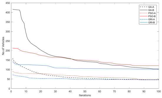
Figure 4.
Comparison of the number of vehicles between GA, PSO, and GRI.
Table 4 presents 1 h output after GRI optimization. It can be seen that the optimization results in each phase in a cycle and the GRI algorithm can be used to obtain a more reasonable signal timing and improve the traffic capacity of the intersection compared with the existing conditions (see Table 3). Seven seconds more cycle length for intersection A was calculated by the GRI algorithm, with phases 1 and 4 increased by 5 s and 4 s, respectively, and phases 2 and 3 decreased by 1 s each. In the case of intersection B, 18 s longer cycle length was proposed with phase 1 increasing by 2 s, phase 2 the same, and phases 3 and 4 increasing by 3 s each compared with existing signal conditions. Thus, concerning queuing, reductions of 10.1% for intersection A and 16.5% for intersection B were achieved by the GRI algorithm.
Table 4.
One-hour cycle length, phase time, and the number of vehicles after GRI optimization.
Figure 5 presents the optimized output by GRI and shows the change in the number of vehicles in the queue (all approaches) over 5 min intervals corresponding to cycle length and phase time. It can be seen that the number of vehicles on all approaches fluctuated.
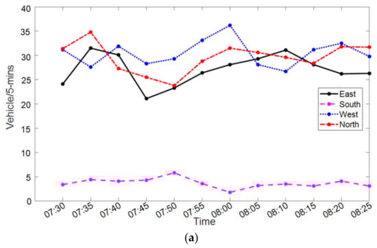
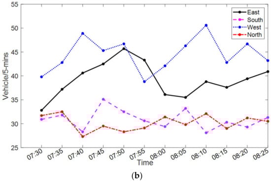
Figure 5.
The number of vehicles in the queue in each approach. (a) Intersection A; (b) Intersection B.
5.2. SIDRA Calibration and Validation with RMSE and GEH
The GRI signal timing application by SIDRA helped to obtain a variety of outputs. Therefore, this work conducted the model calibration and validation based on a relation between the GRI and SIDRA. The number of vehicles in the queue on each approach was compared for every 5 min interval. The data from intersections A and B were used for calibration and validation, respectively. At the stage of calibration and validation, model reliability was obtained by statistical tests, namely, RMSE and GEH.
To ensure integrity and accuracy, before performing calibration of the model whose base data were traffic volumes, speed on the road, and the number of vehicles in the queue, the model was carefully checked to have the same field data of geometry, volumes, speeds, grade, distance between intersections, and signal timings. In addition, cycle length and phase time by GRI were applied to SIDRA (see Table 4).
Table 5 summarizes the results of the three statistical tests. In terms of RMSE assessment, 1.08, 0.46, 3.76, and 0.20 fit were achieved on the eastern, southern, western, and northern approaches, respectively. Moreover, a maximum GEH of 0.57 on the western approach and a minimum GEH of 0.10 on the northern approach were calculated in the GEH procedure, and less than five GEH values were obtained. As a result of the two tests, it is believed that the SIDRA output can reflect the proposed model properly.
Table 5.
RMSE and GEH between GRI and SIDRA: intersection A.
The SIDRA output matches the GRI output closely, and Table 6 presents the results of statistical tests for intersection B. The RMSE was calculated in the range of 0.63–4.64, and the GEH values between 0.09 and 0.69 were computed on all approaches.
Table 6.
RMSE and GEH between GRI and SIDRA: intersection B.
After the application of the optimized signal timing by GRI, the model output shows suitable fitness with SIDRA analysis based on field data. Thus, SIDRA can be used for further intersection analysis based on the optimized signal timing by GRI.
5.3. Capacity, Travel Speed, Vehicle Delay, and CO2
An analytical model, SIDRA, is used for more interesting and comprehensive analysis, which consists of the capability to deduce various results, including capacity, travel speed, average delay, and CO2 emission. Figure 6 compares the analysis results before (current signal timing) and after (optimized signal timing by GRI) at intersection A. In Figure 6a, capacity on the eastern and northern approaches decreased slightly; however, in terms of the entire intersection, capacity was increased by 6.5%. Travel speed on the southern approach was decreased by 1.2%, whereas the total travel speed was increased by 12.2% (see Figure 6b). In contrast, the application of the GRI optimization results can decrease average delay by 17.3% and CO2 emission by 15.6% on the entire intersection as, shown in Figure 6c,d.
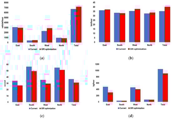
Figure 6.
Further analysis for intersection A. (a) Capacity; (b) Travel speed; (c) Average delay; (d) CO2 emission.
Regarding intersection B, capacity and travel speed on each approach increased after the application of optimized signal timing, as presented in Figure 7a,b. Thus, it was analyzed that there were 7.7% capacity and 9.3% travel speed recorded as increase effect. In addition, the optimized GRI signal timing can decrease average delay by 12.5% and CO2 emission by 11.8%, as depicted in Figure 7c,d.
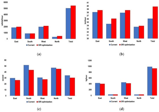
Figure 7.
Further analysis for intersection B. (a) Capacity; (b) Travel speed; (c) Average delay; (d) CO2 emission.
6. Conclusions and Future Works
This paper proposes the GRI algorithm for optimizing cycle length and signal phase time to reduce queues based on two connected intersections with different phase sequences. The results show that the GRI algorithm can find the optimum cycle length and signal phase time, and it can decrease by 10.1% (intersection A) and 16.5% (intersection B) the number of vehicles in the queue compared with the current intersection conditions. In addition, the proposed GRI showed better performance compared with PSO regarding accuracy and with GA regarding speed. Thus, the use of an adaptive GRI algorithm for signal control and timing optimization can reasonably allocate signal cycles, significantly reduce the number of vehicles waiting at intersections, and improve traffic capacity at intersections. Moreover, SIDRA demonstrated that the optimized GRI can increase capacity by 6.5% at intersection A and 7.7% at intersection B. Furthermore, it found that the two intersections have an improving effect on the travel speed and reduced the average delay and CO2 emission. In detail, travel speed increased by 12.2% and 9.3% at intersections A and B, respectively. Additionally, 17.3% (intersection A) and 12.5% (intersection B) of vehicle delay decreased, and 15.6% (intersection A) and 11.8% (intersection B) of CO2 reduced.
In order to minimize traffic congestions at signalized intersections, it is expected that this study will contribute as a platform for future studies that may be more in-depth and focus on the number of vehicles in queues. However, there are also some limitations, and differing phase numbers, sequences, and geometric features, especially road slope, need to be considered. Considering the optimization of the cycle length and phase time, the diverse cases will be taken into account for future studies. In addition, the proposed method can be compared with other improved intelligent traffic signal algorithms based on data collected for longer periods.
Author Contributions
Data curation, H.K.A. and M.A.J.; Formal analysis, M.A.J., G.B., N.Z., A.S.M.M. and F.N.; Funding acquisition, A.S.M.M.; Investigation, H.K.A., G.B., N.Z., A.S.M.M. and M.S.J.; Methodology, G.B. and N.Z.; Project administration, N.Z., P.B. and M.S.J.; Resources, N.Z., P.B. and M.S.J.; Software, H.K.A., M.A.J., N.Z., P.B. and F.N.; Visualization, F.N.; Writing—original draft, H.K.A., M.A.J. and M.S.J.; Writing—review & editing, P.B. All authors have read and agreed to the published version of the manuscript.
Funding
This work was funded by the Researchers Supporting Project No. (RSP-2021/363), King Saud University, Riyadh, Saudi Arabia.
Institutional Review Board Statement
Not applicable.
Informed Consent Statement
Not applicable.
Data Availability Statement
Specific data can be provided upon request.
Conflicts of Interest
On behalf of all the authors, the corresponding author states that there are no conflicts of interest.
References
- Arel, I.; Liu, C.; Urbanik, T.; Kohls, A. Reinforcement learning-based multi-agent system for network traffic signal control. IET Intell. Transp. Syst. 2010, 4, 128–135. [Google Scholar] [CrossRef]
- Nair, A.S.; Liu, J.C.; Rilett, L.; Gupta, S. Non-linear analysis of traffic flow. In Proceedings of the ITSC 2001, IEEE Intelligent Transportation Systems. Proceedings (Cat. No. 01TH8585), Oakland, CA, USA, 25–29 August 2001; IEEE: Piscataway, NJ, USA, 2001. [Google Scholar] [CrossRef]
- Khadhir, A.; Vanajakshi, L.D.; Bhaskar, A. A Microsimulation-Based Stochastic Optimization Approach for Optimal Traffic Signal Design. Transp. Dev. Econ. 2020, 6, 19. [Google Scholar] [CrossRef]
- Sun, L.; Tao, J.; Li, C.; Wang, S.; Tong, Z. Microscopic Simulation and Optimization of Signal Timing based on Multi-Agent: A Case Study of the Intersection in Tianjin. KSCE J. Civ. Eng. 2018, 22, 3373–3382. [Google Scholar] [CrossRef]
- Camagni, R.; Gibelli, M.C.; Rigamonti, P. Urban mobility and urban form: The social and environmental costs of different patterns of urban expansion. Ecol. Econ. 2002, 40, 199–216. [Google Scholar] [CrossRef]
- Goodwin, P.B. Empirical evidence on induced traffic. Transportation 1996, 23, 35–54. [Google Scholar] [CrossRef]
- Hymel, K. If you build it, they will drive: Measuring induced demand for vehicle travel in urban areas. Transp. Policy 2019, 76, 57–66. [Google Scholar] [CrossRef]
- Webster, F. Traffic Signal Settings, Road Research Technical Paper No. 39, Road Research Laboratory; Her Majesty Stationary Office: London, UK, 1958. [Google Scholar]
- Akçelik, R. Traffic Signals: Capacity and Timing Analysis; Australian Road Research Board: Melbourne, VIC, Australia, 1981. [Google Scholar]
- Karoonsoontawong, A.; Waller, S.T. Integrated network capacity expansion and traffic signal optimization problem: Robust bi-level dynamic formulation. Netw. Spat. Econ. 2010, 10, 525–550. [Google Scholar] [CrossRef]
- Srivastava, S.; Sahana, S.K. Nested hybrid evolutionary model for traffic signal optimization. Appl. Intell. 2017, 46, 113–123. [Google Scholar] [CrossRef]
- Sun, S.; Song, B.; Wang, P.; Dong, H.; Chen, X. Shape optimization of underwater wings with a new multi-fidelity bi-level strategy. Struct. Multidiscip. Optim. 2020, 61, 319–341. [Google Scholar] [CrossRef]
- Ahmed, A.; Mehdi, M.R.; Rizvi, S.M.A.; Fatima, T. Evaluation of existing performance and potential for optimization of traffic signals in Karachi. Arab. J. Sci. Eng. 2019, 44, 8747–8759. [Google Scholar] [CrossRef]
- Tokuda, S.; Kanamori, R.; Ito, T. A modification of the stochastic cell transmission model for urban networks. Int. J. Intell. Transp. Syst. Res. 2017, 15, 73–84. [Google Scholar] [CrossRef]
- Niittymäki, J.; Pursula, M. Signal control using fuzzy logic. Fuzzy Sets Syst. 2000, 116, 11–22. [Google Scholar] [CrossRef]
- Onieva, E.; Milanés, V.; Villagrá, J.; Pérez, J.; Godoy, J. Genetic optimization of a vehicle fuzzy decision system for intersections. Expert Syst. Appl. 2012, 39, 13148–13157. [Google Scholar] [CrossRef]
- Khooban, M.H.; Vafamand, N.; Liaghat, A.; Dragicevic, T. An optimal general type-2 fuzzy controller for Urban Traffic Network. ISA Trans. 2017, 66, 335–343. [Google Scholar] [CrossRef]
- Royani, T.; Haddadnia, J.; Alipoor, M. Control of traffic light in isolated intersections using fuzzy neural network and genetic algorithm. Int. J. Comput. Electr. Eng. 2013, 5, 142–146. [Google Scholar] [CrossRef]
- Araghi, S.; Khosravi, A.; Creighton, D. Comparing the performance of different types of distributed fuzzy-based traffic signal controllers. J. Intell. Fuzzy Syst. 2019, 36, 6155–6166. [Google Scholar] [CrossRef]
- Jabbarpour, M.R.; Zarrabi, H.; Khokhar, R.H.; Shamshirband, S.; Choo, K.K.R. Applications of computational intelligence in vehicle traffic congestion problem: A survey. Soft Comput. 2018, 22, 2299–2320. [Google Scholar] [CrossRef]
- Ceylan, H.; Bell, M.G. Traffic signal timing optimisation based on genetic algorithm approach, including drivers’ routing. Transp. Res. Part B Methodol. 2004, 38, 329–342. [Google Scholar] [CrossRef]
- Turky, A.M.; Ahmad, M.S.; Yusoff, M.Z.M. The use of genetic algorithm for traffic light and pedestrian crossing control. Int. J. Comput. Sci. Netw. Secur. 2009, 9, 88–96. [Google Scholar]
- Odeh, S.M. Management of an intelligent traffic light system by using genetic algorithm. J. Image Graph. 2013, 1, 90–93. [Google Scholar] [CrossRef]
- Liu, M.; Oeda, Y.; Sumi, T. Multi-Objective Optimization of Intersection Signal Time Based on Genetic Algorithm. Mem. Fac. Eng. Kyushu Univ. 2018, 78, 14–23. [Google Scholar]
- Possel, B.; Wismans, L.J.J.; Van Berkum, E.C.; Bliemer, M.C.J. The multi-objective network design problem using minimizing externalities as objectives: Comparison of a genetic algorithm and simulated annealing framework. Transportation 2018, 45, 545–572. [Google Scholar] [CrossRef]
- Guo, J.; Kong, Y.; Li, Z.; Huang, W.; Cao, J.; Wei, Y. A model and genetic algorithm for area-wide intersection signal optimization under user equilibrium traffic. Math. Comput. Simul. 2019, 155, 92–104. [Google Scholar] [CrossRef]
- Renfrew, D.; Yu, X.H. Traffic signal control with swarm intelligence. In Proceedings of the 2009 Fifth International Conference on Natural Computation, Tianjin, China, 14–16 August 2009; IEEE: Piscataway, NJ, USA, 2009. [Google Scholar] [CrossRef]
- García-Nieto, J.; Olivera, A.C.; Alba, E. Optimal cycle program of traffic lights with particle swarm optimization. IEEE Trans. Evol. Comput. 2013, 17, 823–839. [Google Scholar] [CrossRef]
- Wijaya, I.G.P.S.; Uchimura, K.; Koutaki, G. Traffic light signal parameters optimization using particle swarm optimization. In Proceedings of the 2015 International Seminar on Intelligent Technology and Its Applications (ISITIA), Surabaya, Indonesia, 20–21 May 2015; IEEE: Piscataway, NJ, USA, 2015. [Google Scholar] [CrossRef]
- Jia, H.; Lin, Y.; Luo, Q.; Li, Y.; Miao, H. Multi-objective optimization of urban road intersection signal timing based on particle swarm optimization algorithm. Adv. Mech. Eng. 2019, 11, 1687814019842498. [Google Scholar] [CrossRef]
- Shaikh, P.W.; El-Abd, M.; Khanafer, M.; Gao, K. A review on swarm intelligence and evolutionary algorithms for solving the traffic signal control problem. IEEE Trans. Intell. Transp. Syst. 2020, 23, 48–63. [Google Scholar] [CrossRef]
- Jafari, S.; Shahbazi, Z.; Byun, Y.-C. Designing the Controller-Based Urban Traffic Evaluation and Prediction Using Model Predictive Approach. Appl. Sci. 2022, 12, 1992. [Google Scholar] [CrossRef]
- Jafari, S.; Shahbazi, Z.; Byun, Y.-C. Signal Traffic Optimization Using Control Algorithm in Urban Traffic Framew. Turk. J. Comput. Math. Educ. 2022, 13, 803–819. [Google Scholar]
- Gao, K.; Zhang, Y.; Sadollah, A.; Lentzakis, A.; Su, R. Jaya, harmony search and water cycle algorithms for solving large-scale real-life urban traffic light scheduling problem. Swarm Evol. Comput. 2017, 37, 58–72. [Google Scholar] [CrossRef]
- Ferrer, J.; López-Ibáñez, M.; Alba, E. Reliable simulation-optimization of traffic lights in a real-world city. Appl. Soft Comput. 2019, 78, 697–711. [Google Scholar] [CrossRef]
- Qadri, S.S.S.M.; Gökçe, M.A.; Öner, E. State-of-art review of traffic signal control methods: Challenges and opportunities. Eur. Transp. Res. Rev. 2020, 12, 55. [Google Scholar] [CrossRef]
- An, H.K.; Yue, W.L.; Stazic, B. Dual signal roundabout evaluation in Adelaide using SIDRA and AIMSUN. Road Transp. Res. A J. Aust. N. Z. Res. Pract. 2017, 26, 36–49. [Google Scholar]
- Akmaz, M.M.; Çelik, O.N. Examination of Signalized Intersections According to Australian and HCM (Highway Capacity Manual) Methods Using Sidra Intersection Software. J. Civ. Eng. Arch. 2016, 10, 246–259. [Google Scholar] [CrossRef][Green Version]
- Pitsiava-Latinopoulou, M.; Mustafa, M.A. The Accuracy of Estimating Delay at Signalized Intersections: A Comparison Between Two Methods. Traffic Eng. Control 1992, 33, 306–311. [Google Scholar]
- Chai, T.; Draxler, R.R. Root mean square error (RMSE) or mean absolute error (MAE)? Arguments against avoiding RMSE in the literature. Geosci. Model Dev. 2014, 7, 1247–1250. [Google Scholar] [CrossRef]
- Xevi, E.; Christiaens, K.; Espino, A.; Sewnandan, W.; Mallants, D.; Sørensen, H.; Feyen, J. Calibration, validation and sensitivity analysis of the MIKE-SHE model using the Neuenkirchen catchment as case study. Water Resour. Manag. 1997, 11, 219–242. [Google Scholar] [CrossRef]
- Mentaschi, L.; Besio, G.; Cassola, F.; Mazzino, A. Problems in RMSE-based wave model validations. Ocean Model. 2013, 72, 53–58. [Google Scholar] [CrossRef]
- Dewees, D.N. Estimating the time costs of highway congestion. Econom. J. Econom. Soc. 1979, 47, 1499–1512. [Google Scholar] [CrossRef]
- Paz, A.; Molano, V.; Gaviria, C. Calibration of CORSIM models considering all model parameters simultaneously. In Proceedings of the 15th International IEEE Conference on Intelligent Transportation Systems, Anchorage, AK, USA, 16–19 September 2012. [Google Scholar]
- Vasconcelos, L.; Silva, A.B.; Seco, A.; Silva, J.P. Estimating the parameters of Cowan’s M3 headway distribution for roundabout analyses. Balt. J. Road Bridge Eng. 2012, 7, 216–268. [Google Scholar] [CrossRef]
- Vuk, G.; Hansen, C.O. Validating the Passenger Traffic Model for Copenhagen. Transportation 2006, 33, 371–392. [Google Scholar] [CrossRef]


Publisher’s Note: MDPI stays neutral with regard to jurisdictional claims in published maps and institutional affiliations. |
© 2022 by the authors. Licensee MDPI, Basel, Switzerland. This article is an open access article distributed under the terms and conditions of the Creative Commons Attribution (CC BY) license (https://creativecommons.org/licenses/by/4.0/).