Mathematical Model for the Generalized VRP Model

Abstract

The Vehicle Routing Problem (VRP) is a highly investigated logistics problem. VRP can model in-plant and out-plant material handling or a whole supply chain. The first Vehicle Routing Problem article was published in 1959 by Dantzig and Ramser, and many varieties of VRP have appeared since then. Transport systems are becoming more and more customized these days, so it is necessary to develop a general system that covers many transport tasks. Based on the literature, several components of VRP have appeared, but the development of an integrated system with all components has not yet been completed by the researchers. An integrated system can be useful because it is easy to configure; many transportation tasks can be easily modeled with its help. Our purpose is to present a generalized VRP model and show, in the form of case studies, how many transport tasks the system can model by including (omitting) each component. In this article, a generalized system is introduced, which covers the main VRP types that have appeared over the years. In the introduction, the basic Vehicle Routing Problem is presented, where the most important Vehicle Routing Problem components published so far are also detailed. The paper also gives the mathematical model of the generalization of the Vehicle Routing Problem and some case studies of the model are presented.

1. Introduction

The first article on the Vehicle Routing Problem was published in 1959 by Dantzig and Ramser [1]. Since then, many researchers presented some task types related to different industrial transportation needs. In the following, we outline the classic Vehicle Routing Problem (VRP), i.e., the simplest VRP.

Figure 1 illustrates the classic Vehicle Routing Problem, where the positions and product demands of the customers are given. The position of a depot is also known in advance. The numbers of the vehicle and their capacity limits are also given. The vehicles deliver the products from the depot to the customers and then return to the depot. In a classic VRP, the objective is to minimize the distance travelled by the vehicles. In Figure 1, 14 customers are served by 4 vehicles.

The types of Vehicle Routing Problem used in the literature are classified into major categories according to the main component involved in the Vehicle Routing Problem model. The following main components are distinguished: node, vehicle, time, product, cost, value type and functional parameter. We summarized the main VRP problem types in

Table 1. Main VRP types.

Name	Description
Node Component
Traveling Salesman Problem [2]	A single agent (vehicle) visits the cities (customers). The vehicle makes a trip. The objective is to minimize the distance the vehicle travels. Cities (customers) have no product demand
Vehicle Routing Problem with Single Depot [3]	The vehicles leave a common depot, visit the customers (deliver products to the customers) and then return to the depot (after the customers have visited).
Vehicle Routing Problem with Multiple Depot [4]	The system includes several depots, each vehicle starts their route from one of the depots and then returns there at the end of their route.
Two-Echelon Vehicle Routing Problem [5]	The products are first transported from the depot to intermediate locations (satellites) and then onwards to customers. Movements of products between a depot-satellite and a satellite-customer can be made by different types of (capacity-constrained) vehicles. Thus, depot-satellite vehicles have a higher capacity limit and satellite-customer vehicles have a lower capacity limit.
Vehicle Routing Problems with Traffic Congestion [6]	The time between each node (depots, satellites, customers) also depends on the traffic. The objective is for vehicles to make their route as soon as possible.
Risk Constrained Vehicle Routing Problem [7]	The road safety between the individual nodes (depots, satellites, customers) was also given. The objective is for vehicles to travel as safely as possible.
Risk-constrained Cash-in-Transit Vehicle Routing Problem [8]	This problem is similar to the Risk Constrained Vehicle Routing Problem, but here cash-in-transit vehicles travel
Vehicle component
Homogeneous Fleet Vehicle Routing Problem [9]	The system includes vehicles of the same type.
Heterogeneous Fleet Vehicle Routing Problem [9]	The system includes different types of vehicles.
Capacitated Vehicle Routing Problem [3]	The vehicles have a capacity constraint on the products.
Environmentally Friendly Vehicle Routing Problem [10]	The vehicles are of an environmentally friendly type.
Electric Vehicle Routing Problem [11]	Electric vehicles travel, the vehicles visit recharger stations after a certain distance.
Fuel Efficient Green Vehicle Routing Problem [12]	The objective is to minimize fuel emissions from vehicles.
Vehicle Routing Problem with Occasional Drivers [13]	If the company is unable to deliver the products with its fleet of vehicles, it can also use rented vehicles to meet the goods needs of the customers.
Time component
Vehicle Routing Problem with Time Window [14]	Customers may have different time windows. The product demands of the customers must be served within the time window. The customer can have single or multiple time window.
Vehicle Routing Problem with Multiple Time Windows [15]	Multiple time windows have been added to customers. The product demands of the customers must be satisfied within a time window.
Vehicle Routing Problem with Soft Time Window [16]	The demands of the customers can be met outside the time window, but then there is a penalty point.
Periodic Vehicle Routing Problem [17]	Customers do not have to be visited once, but periodically, even several times within a (predefined) period.
Cumulative Capacitated Vehicle Routing Problem [18]	The objective is to minimize latency at the nodes.
Vehicle Routing Problem with Perishable Food Products Delivery [19]	Perishable products are delivered, so the expiration date of the products must also be taken into account.
Product component
Vehicle Routing Problem with Multiple Product [20]	There are several types of products in the system. This means that each customer may have multiple product demands.
Cost component
Selective Vehicle Routing Problem [21]	Not all demands of the customers are satisfied, only those that are profitable.
Functional parameter component
Open Vehicle Routing Problem [22]	One or more depots are in the system from which vehicles departed to visit customers. However, the vehicles after visit the customers do not return to the depot.
Multi-Depot Vehicle Routing Problem with Inter-Depot Routes [23]	One or more depots are in the system from which vehicles departed to visit customers. Once the customers are visited, vehicles can return to any depot.
Vehicle Routing Problem with Pickup and Delivery [24]	Not only the delivery but also the collection (pickup) of products is important.
Vehicle Routing Problem with Cross-Docking [25]	The collected products are not stored for a long time, almost immediately after the pick-up, delivery phase begins.
Value parameter component
Static value	The value is given by a real number.
Fuzzy Vehicle Routing Problem [26]	Some factors, e.g., time window, demand for products, the distance between nodes, etc. given with fuzzy numbers.
Stochastic Vehicle Routing Problem [27]	Some factors, e.g., time window, demand for products, the distance between nodes, etc. given with a probability distribution.

.

In the literature, we can find many complex systems, however, even these articles were limited to only one specific type of transportation task (e.g., transportation by electric cars, multilevel transportation). Regarding new contributions, we can highlight the following topics.

The solution of electric VRP is reported in [28], where the task included the following basic components: customers, recharging stations, vehicles (EVs), depot and recharging stations. The following constraint factors, criteria and objective function components were used: distance from the locations, travel time from the locations, demand of the customer, service time, time window, time limit of the route, capacity limit of the vehicles, cargo capacity of the vehicles, battery capacity, fuel consumption, battery recharging, driver wage, vehicle acquisition. The objective function is the minimization of the distance, driver wage and vehicle acquisition.

The authors of [29] present a model that includes the following components: depot, customers, several vehicles and one type of product. The following limits and other components are included in the system: time window, renewable resource, consumable resource, vehicle capacity limit, service time in node, distance from node, travel time from the node and node demand.

In [30], multi-objectives multi-depot VRPs are analyzed. The authors used the following basic components: homogeneous vehicles, customers, depots, the distance between nodes, multiple product types, product price, emission produced by the vehicle, travel time between nodes, unloading and loading time at nodes and transportation cost. The capacities of vehicles were also contained in the problem.

Green VRP is presented by the authors [31]. The following main components were used: customer, depot and homogeneous vehicles. The following constraints and components were also applied: demand at the node, the distance between the nodes, the capacity of the vehicles, traveling speed and time between the nodes and time window of the service.

A 2E-VRP system is presented by the authors [32]. In the article, depot, satellite and customer were used. The following components were used: demand of customer, distance from nodes, time window of customers, vehicles capacity, handling cost per unit, transportation cost, vehicle speed and fuel cost.

A multi-cost system is also presented in the following article [33]. Here, the system includes customers and a single depot. The distance and time of the route between nodes matters. There are different types of vehicles with different capacities. Customer demand is also important. There are two types of customer, one that is light load and the other, which can be used at any time.

Based on the presented systems, it can be said that certain factors are members of almost all systems. These are depots, customers, vehicles (heterogeneous or homogeneous) one or more types of products, customers’ demand for products, time window, and distance between nodes.

2. The Mathematical Model of the Generalization of the Vehicle Routing Problem

The purpose of this chapter is to present a mathematical model of the generalized Vehicle Routing Problem. The generalized system presented here includes the systems listed in the review. Our system is such that by properly configuring the components (omitting them, i.e., setting the values to 0), we can get the systems in the literature review.

To describe the mathematical model the following notations are used:

• $i$: level index
• $j$: position index (positions within the level)
• $t$: time in a period
• $k$: vehicle index (vehicles within the level)
• $m$: product index
• $n$: stochastic value index
• $p$: forecasted value index
• $q$: time window index
• $M$: positive large constant
• $a$: start time of node service
• $b$: arrival time at the node
• $d$: time window penalty point

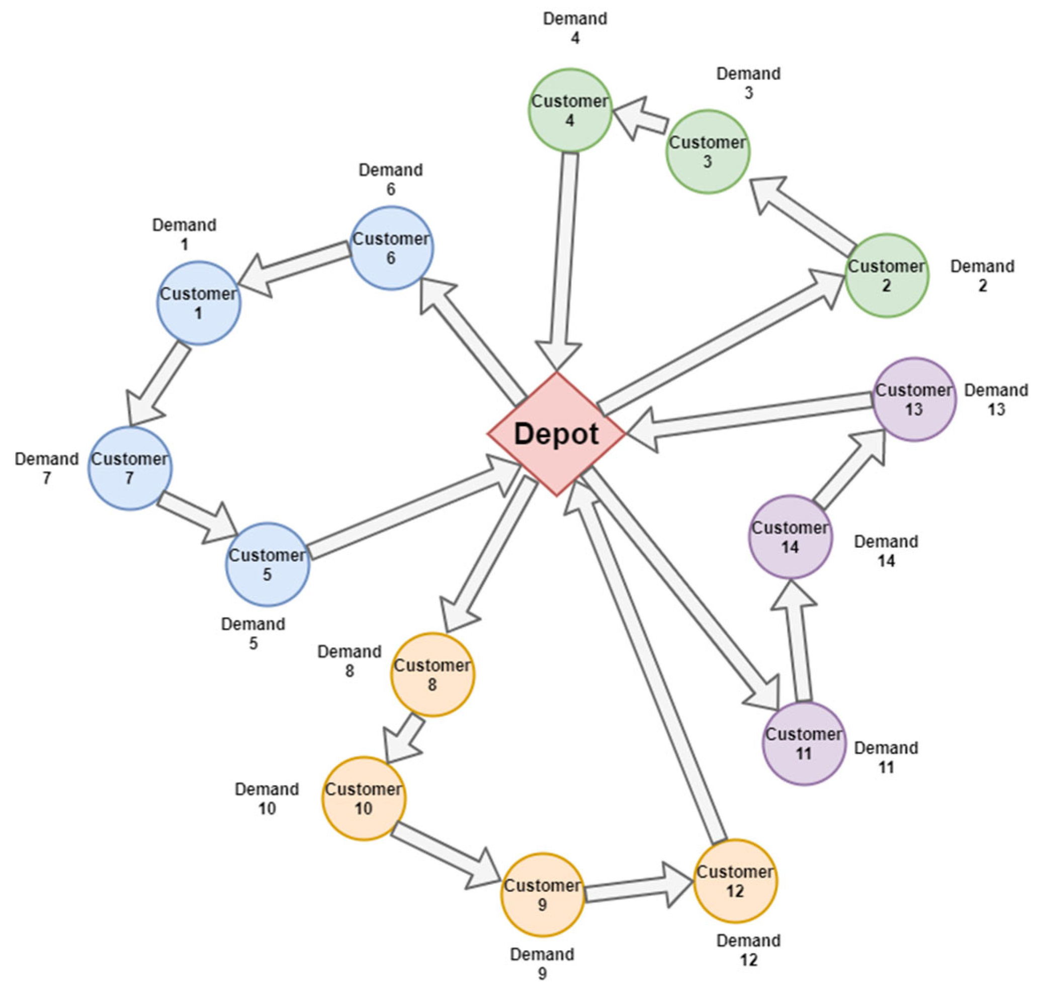
2.1. Topology Graph Description

The topology of the Vehicle Routing Problem can be described by a graph. Nodes denote positions (customers, depots, etc.) and edges denote transport relationships between positions.

The graph contains the nodes and the relationships between them. Several levels are assumed in the graph. The set of the levels can be written in the following way:

$$LEVEL=\left\{leve{l}_1,\dots ,leve{l}_{n_{level}}\right\}$$

(1)

The first level contains only depots, the intermediate levels are local service centres (satellites) and the last level is customers. The levels indicate the direction of the transportation of products. Usually, products are transported from the higher level to the lower level. This is the case with delivery. The case of pick-up is when products are transported from a lower level to a higher level. The intermediate levels are called satellites. The use of intermediate levels can be useful in many cases, such as in the post office, where letters are transferred from a central sorter to an additional area sorter. Different vehicle types can be used at the intermediate levels, thus reducing transportation costs.

The number of levels is denoted by $n_{level}$. In this case, the graph $G$ of the model can be written as follows:

$$G=\left\{G_i\right\},\hspace{1em}\hspace{1em}i=1\dots n_{level}$$

(2)

where

$$G_i=\left\{PO{S}_i,RE{L}_i\right\}$$

(3)

$PO{S}_i$ denotes the positions, and $RE{L}_i$ denotes the relations between the positions.

There can be several relations between nodes, which can change over time:

$$RE{L}_i\subseteq PO{S}_i\times PO{S}_i$$

(4)

Then, each position is denoted by the symbol $po{s}_j^i$, where $i$ denotes the level and $j$ denotes the sequence number index within the level.

$$PO{S}_i=\left\{po{s}_1^i,\dots ,po{s}_{no{l}_i}^i\right\}$$

(5)

The set of all positions for the entire model graph:

$$POS=\underset{i}{{\displaystyle \cup }}PO{S}_i$$

(6)

and the number of positions:

$$n_{position}=\left|POS\right|.$$

(7)

2.2. Vehicles

The transportation of products is carried out by vehicles. Different types of vehicles can be used in the system. The number of vehicle types is denoted by $n_{vehicletype}$.

The possible vehicle types are described globally in the following way:

$$VEHICLE=\left\{vehicl{e}_1,\dots ,vehicl{e}_{n_{vehicletype}}\right\}$$

(8)

The number of vehicles varies by level and type, their values are described by

$$CNTVEHICLE=\left\{cntvehicl{e}_k^i\right\}$$

(9)

All vehicles in the system are marked with

$$n_{vehicle}={\displaystyle \sum }_i{\displaystyle \sum }_{k}cntvehicl{e}_k^i$$

(10)

2.3. Products, Services

Vehicles can transport products from one node to another. The products greatly influence the values of the individual components, such as the product demands of the nodes, whether a certain product can be delivered with a certain vehicle, the capacity constraint of the vehicles, which products can be delivered together, and so on.

In the model, several different products are delivered. The number of product types is specified with $n_{producttype}$.

The possible types of products are indicated globally with

$$PRODUCT=\left\{produc{t}_1,\dots ,produc{t}_{n_{producttype}}\right\}$$

(11)

2.4. Time

Period time means a certain time interval. This time interval is divided into units of the same size. For example, the period time can be the day and the time unit may be one hour, so the day is divided into 24 h. Period time is important because certain deliveries do not have to be made once, but continuously, periodically. This factor can be important for any transportation task, as most deliveries do not occur once, but with some regularity.

So, there are repeating parts that consist of $n_{period}$ atomic time units. This can be written in the following way:

$$TIME=\left\{tim{e}_1,tim{e}_2,\dots ,tim{e}_{n_{period}}\right\}$$

(12)

Attributes (properties) can be assigned to the building blocks of the model. Based on the value set, in the following, the attribute types are presented.

2.5. Values

Static value: Static value means, that the value is known exactly. $VALUE$ is a real number, so $VALUE\in {ℝ}^{+}$.

Stochastic value: The stochastic value indicates that the values of the components take on the values with some probability, so $VALUE=\left\{valu{e}_1,valu{e}_2,\dots ,valu{e}_n\right\}$, where $k$ indicates the number of values for each $\left(po{s}_j^i,po{s}_j^i\right)$ arc. $valu{e}_n=\left\{real\_numbe{r}_n,probabilit{y}_n\right\}$, where $real\_number\in {ℝ}^{+}, probability\in \left\{0,1\right\}$, and ${{\displaystyle \sum }}^{}probability=1$

Fuzzy value: The values of the components are given in fuzzy numbers, in the following way:

$$\mathrm{VALUE}=\left\{numbe{r}_1,numbe{r}_2,numbe{r}_3,numbe{r}_4\right\}\mathrm{where}number\in {ℝ}^{+}$$

Forecasted: Only past data are given. So, the values and the dates (times) are given, which can be written in the following:

$VALUE$ is forecasted from the following set $\left\{valu{e}_1,valu{e}_2,\dots ,valu{e}_p\right\}$, where $valu{e}_p=\left\{tim{e}_p,real\_numbe{r}_p\right\}$, $real\_number\in {ℝ}^{+}$.

Based on the meaning, several attributes can be defined. The attributes can be divided into the following main groups: node, vehicle, time, product, cost, functional parameters. The attributes have the main group and can belong to another group.

2.6. The Attributes of the Node Main Group

In the following, the attributes of the node group are presented.

Table 2. The attributes of the node main group.

Attribute Name	Notation	Short Notation	Dependency	Value Type
Travel time between the nodes	$TTBN\left(i_1,j_1, i_2,j_2,vehicl{e}_k,t\right)$	$TTBN$	$i_1,j_1$: the starting node $i_2,j_2$: the ending node $vehicl{e}_k$: the vehicle type $t$: the time	static, stochastic, fuzzy, forecasted
Travel distance between the nodes	$TDBN\left(i_1,j_1, i_2,j_2,vehicl{e}_k,t\right)$	$TDBN$
Reliability between the nodes	$RBN\left(i_1,j_1, i_2,j_2,vehicl{e}_k,t\right)$	$RBN$
Route status between the nodes	$RSBN\left(i_1,j_1, i_2,j_2,vehicl{e}_k,t\right)$	$RSBN$
Type of the node	$TN\left(i_1,j_1\right)$	$TN$	$i_1,j_1$: the node	CUSTOMER, DEPOT, SATELLITE, RECHARGERSTATION

indicates the attributes of the node main group. This group has 6 attributes. The dependencies of most attributes are as follows: the starting node, the ending node, the vehicle and the time. Additionally, their value type can be static stochastic fuzzy or forecasted. Only the type of the node attribute has only the node dependency. The value of this attribute can be customer, depot, satellite or recharger station. In the following, we demonstrate why these parameters may be important in transport tasks.

The travel time between nodes does not match the distance between nodes. Although it is related because longer travel time is required between farther nodes than between closer nodes, other factors can also affect time, such as road quality, speed limits in the city, traffic lights, and so on.

Travel distance between the nodes: distance is a very important factor, as the time of service (travel time between nodes), the fuel consumed and thus the cost of service is highly dependent on the distance between two nodes.

Reliability between the nodes: By reliability, we mean robbery reliability. It is not worth transporting on a route where there is a high risk of robbery, as we risk the products being transported and the safety of the driver.

Route status between the nodes: This increases the delivery time and the depreciation of the vehicles, thus reducing the profit, so it is worthwhile to follow the best possible route if the detour is not too long.

Type of the node: The following types are distinguished in our model: CUSTOMER, DEPOT, SATELLITE, RECHARGERSTATION. The transportation problem defines levels, where the top element of the level is the depot, from where the delivery of the products starts. Satellite refers to intermediate points where products are transported by vehicles and then transported by other types of vehicles to a lower-level satellite or customer. Indirect delivery is good because we can use different types of vehicles; the lower the level, the lower the capacity of the vehicle. The recharger station is important in the case of vehicles; they enter here when the fuel is running out and then continue to visit the customers after refueling.

2.7. The Attributes of the Vehicle Group

In the following, the attributes of the vehicle group are presented.

Table 3. The attributes of the vehicle group.

Attribute Name	Notation	Short Notation	Dependency	Value Type
The capacity constraint	$CCVTPT\left(vehicl{e}_k,produc{t}_m\right)$	$CCVTPT$	$vehicl{e}_k$: vehicle ${product}_m$: product	static, stochastic, fuzzy, forecasted
Fuel consumption	$FC\left(vehicl{e}_k\right)$	$FC$	$vehicl{e}_k$: vehicle
Recharger time	$RTV\left(vehicl{e}_k\right)$	$RTV$
Own vehicle or borrowed vehicle	$OBV\left(vehicl{e}_k\right)$	$OBV$
Rental fee per vehicle types	$RFVT\left(vehicl{e}_k\right)$	$RFVT$
Maximum distance with a full tank	$MDFT\left(vehicl{e}_k\right)$	$MDFT$

indicates the attributes of the vehicle main group. This group has 6 attributes. The dependencies of most attributes are only the vehicle. Additionally, their value type can be static stochastic fuzzy or forecasted. Only the capacity constraint attribute has two dependencies, the vehicle and the product. In the following, we demonstrate, why these parameters may be important in a transport tasks.

The capacity constraint: Each vehicle has a capacity limit for the products to be transported.

Fuel consumption: Each vehicle type may have different fuel consumption. Fuel consumption will be an important factor in the cost of fuel consumption of a vehicle, based on the unit of distance travelled by each vehicle.

Own vehicle or borrowed vehicle: There is a rental fee for rented vehicles, but it may be worthwhile to use such vehicles due to possible fluctuating or seasonal demand when the demand of the customers is unable to satisfy the existing fleet of vehicles. In this case, using the rented vehicles, all demand that arises can be satisfied, so the company do not lose customers.

2.8. The Attributes of the Time Group

In the following, the attributes of the time group are presented.

Table 4. The attributes of the time group.

Attribute Name	Notation	Short Notation	Dependency	Value Type
Service handling time	$SHT\left(i_1,j_1,produc{t}_m,vehicl{e}_k,t\right)$	$SHT$	$i_1,j_1$: the starting node $i_2,j_2$: the ending node $produc{t}_m:$ the product $vehicl{e}_k$: the vehicle type $t$: the time	static, stochastic, fuzzy, forecasted
Packing time	$PT\left(i_1,j_1,produc{t}_m,vehicl{e}_k,t\right)$	$PT$
Unpacking time	$UPT\left(i_1,j_1,produc{t}_m,vehicl{e}_k,t\right)$	$UPT$
Loading time	$LT\left(i_1,j_1,produc{t}_m,vehicl{e}_k,t\right)$	$LT$
Unloading time	$ULT\left(i_1,j_1,produc{t}_m,vehicl{e}_k,t\right)$	$ULT$
Fixed capital time	$FCT\left(i_1,j_1,produc{t}_m,vehicl{e}_k,t\right)$	$FCT$
Administration time	$AT\left(i_1,j_1,produc{t}_m,vehicl{e}_k,t\right)$	$AT$
Quality control time	$QCT\left(i_1,j_1,produc{t}_m,vehicl{e}_k,t\right)$	$QCT$
Time window	$TW\left(i_1,j_1,produc{t}_m,t\right)$	$TW$	$i_1,j_1$: the starting node $i_2,j_2$: the ending node $produc{t}_m:$ the product $t$: the time	$\left\{\left[tw{e}_1, tw{l}_1\right],\dots \begin{array}{c}\left[tw{e}_q, tw{l}_q\right]\end{array}\right\}$ $tw{e}_q \left(\mathrm{earliest}\mathrm{time}\right), tw{l}_q$(latest time) can be static, stochastic, fuzzy, forecasted

indicates the attributes of the time main group. This group has 9 attributes. Service handling time: In the case of handling a service, vehicles have to spend some time at the customer, until the service is completed. Packing time: The products are packed before transportation. Each type of product has a different packing time for each node. It may depend on the type of product because each type of product requires different packing. Unpacking time: It may be necessary to unpack individual products at intermediate locations (satellites) and then transport them from there with another package. Loading and unloading time: Different types of products require loading times of different durations, and it does not matter what kind of resource the machine has (machines, human resources). Fixed capital time: Fixed capital time means that the product is waiting at intermediate locations (satellites). Administration time: The administration time depends on the node, the type of products and the time. In each position, the human resources may be different at each time, e.g., at night, less human resources than in the morning, early afternoon hours. Time window: It depends on the node because each node can have, e.g., their opening hours, time of receipt of products or, in the case of in-plant transport, the production time interval of each production site. It depends on the products to be delivered because each position is, e.g., within the production time interval; they only need the individual products, semi-finished products, or raw materials at a certain time (time window).

2.9. The Attributes of the Product Group

In the following, the attributes of the product group are presented.

Table 5. The attributes of the product group.

Attribute Name	Notation	Short Notation	Dependency	Value Type
The capacity constraint of the node	$CCN\left(i_1,j_1,produc{t}_m,t\right)$	$CCN$	$i_1,j_1$: the starting node $i_2,j_2$: the ending node $produc{t}_m:$ the product $t$: the time	static, stochastic, fuzzy, forecasted
Product demand of the node	$PDN\left(i_1,j_1,produc{t}_m,t\right)$	$PDN$
Prices of product	$PP\left(i_1,j_1,produc{t}_m,t\right)$	$PP$
Given order of products	$GOPD\left(i_1,j_1,produc{t}_m,t\right)$	$GOPD$		$\left\{0,1,\dots ,noproducttype\right\}$.
Given products handling together	$GPHT\left(i_1,j_1,produc{t}_{m_1},produc{t}_{m_2}\right)$	$GPHT$	$produc{t}_{m_1}:$ one product $produc{t}_{m_2}:$ another product	true, false
Storage level of the locations	$DSSL\left(i_1,j_1,produc{t}_m,t\right)$	$DSSL$	$i_1,j_1$: the starting node $i_2,j_2$: the ending node $produc{t}_m:$ the product $t$: the time	static, stochastic, fuzzy, forecasted

indicates the attributes of the product main group. The capacity constraint of the node: Nodes have a capacity limit for each type of product. So, given how much of each type of products can be stored. Product demand of the node: The demand of the nodes depends on the node, the type of the product, and the time. It depends on the time because the demand for products may be high in one season and low in another. An example of this is the jacket in clothing stores, which is needed in the winter and not in the summer. Prices of product: Each product has a price (value). It depends on the node because the products can be sold at a different price at a different node. It depends on time because each product can be sold at different prices at different times. For example, in the food industry, fruits can be sold more expensive in winter than during the season. Given order of products: This condition means that certain products must be received by the nodes in order. So, after product A, product B must be delivered, and not the other way around. In the case of in-plant transport, it may be a useful condition for transport to the production line, as raw material B may be required after a raw material A, in the reverse order (first B is delivered then A) raw material B requires storage space. Given products handling together: this means whether certain types of products can be shipped with one vehicle at a time. It can be an important factor because certain types of products cannot be shipped with the same vehicle. For example, bread cannot be transported with frozen products, but bread with canned food can. Storage level of the locations: an important factor can be how many products are already in each node.

2.10. The Attributes of the Cost Group

In the following, the attributes of the cost group are presented.

Table 6. The attributes of the cost group.

Attribute Name	Notation	Short Notation	Dependency	Value Type
Packaging costs	$PC\left(i_1,j_1,produc{t}_m,vehicl{e}_k,t\right)$	$PC$	$i_1,j_1$: the starting node $produc{t}_m:$ the product $vehicl{e}_k$: the vehicle $t$: the time	static, stochastic, fuzzy, forecasted
Unpacking cost	$UPC\left(i_1,j_1,produc{t}_m,vehicl{e}_k,t\right)$	$UPC$
Loading costs	$LC\left(i_1,j_1,produc{t}_m,vehicl{e}_k,t\right)$	$LC$
Unloading costs	$ULC\left(i_1,j_1,produc{t}_m,vehicl{e}_k,t\right)$	$ULC$
Administrative costs	$AC\left(i_1,j_1,produc{t}_m,vehicl{e}_k,t\right)$	$AC$
Quality control cost	$QCC\left(i_1,j_1,produc{t}_m,vehicl{e}_k,t\right)$	$QCC$

indicates the attributes of the cost main group.

2.11. The Attributes of the Functional Parameter Group

In the following, the attributes of the functional parameter component are presented.

Table 7. The attributes of the functional parameter group.

Attribute Name	Notation	Short Notation	Dependency	Value Type
Inter-depot route	$IDR(vehicl{e}_k)$	$IDR$	$vehicl{e}_k$: the vehicle	true, false
Delivery	$D\left(i_1,j_1,produc{t}_m\right)$	$D$	$i_1,j_1$: the starting node $produc{t}_m:$ the product
Pickup	$PU\left(i_1,j_1,produc{t}_m\right)$	$PU$
Soft time window	$STW\left(i_1,j_1,produc{t}_m\right)$	$STW$
Open route	$OR\left(vehicl{e}_k\right)$	$OR$	$vehicl{e}_k$: the vehicle

indicates the attributes of the functional parameter main group. Inter-depot route: This parameter describes whether the vehicle should return to the depot (higher-level node) from which it started, or even choose from other depots (other higher-level positions); it is not necessary to return there after visiting the nodes. Delivery: The products are transported from higher levels to smaller levels. This type depends on the node and the type of products. Pickup: In this case, the products are transported from the smaller levels to the larger levels. Soft time window: In the case of this VRP component, exceeding the time window is also allowed, but then a penalty point is introduced. Open route: For this type, although the vehicles start from a node at the above level, it does not return to any node at any of the above levels after visiting the lower-level nodes.

2.12. Decision Variable and Constraints of Our Model

In the following, the decision variable and the constraint of our system is introduced.

(1) 

Decision variable

$${\lambda }_{j_1,j_2}^{i_1,i_2,k,t,m}=\{\begin{array}{c}1, if vehicle k in period t in level i_1 after node j_1 travels to \\ node j_2 in level i_2 immediately \\ and transport product m \\ 0 else\end{array}$$

(13)

In the equation, $i_1,j_1$ determines one of the two nodes and $i_2,j_2$ determines the other node, $k$ is the index of the vehicles, $t$ is the index of the time, and $m$ is the index of products.

(2) 

Constraints

• Constraint 1:

A node at level $i$ only needs to be served once a period by a vehicle with $m$ product. It can be written in the following ways:

$$\begin{gathered} \forall j_2\in POS,\forall i_2\in LEVEL,\forall t\in TIME,\forall m\in PRODUCT: \\ {\displaystyle \sum }_{i_1}^{n_{level}}{\displaystyle \sum }_{j_1=1}^{n_{position}{}_{i_1}}{\displaystyle \sum }_{k=1}^{n_{vehicle}}{\lambda }_{j_1,j_2}^{i_1,i_2,k,t,m}\le 1 \end{gathered}$$

(14)

$$\begin{gathered} \forall j_1\in POS,\forall i_1\in LEVEL,\forall i_2\in LEVEL,\forall t\in TIME,\forall m\in PRODUCT: \\ {\displaystyle \sum }_{i_2}^{n_{level}}{\displaystyle \sum }_{j_2=1}^{n_{position}{}_{i_2}}{\displaystyle \sum }_{k=1}^{n_{vehicle}}{\lambda }_{j_1,j_2}^{i_1,i_2,k,t,m}\le 1 \end{gathered}$$

(15)

• Constraint 2:

The time window of the nodes must be taken into account.

This constraint is optional and should only be considered if a time window has been defined. If a time window is defined, two cases are possible, the hard time window and the soft time window. In the case of a hard time window, the time window must be observed, while in the case of a soft time window it must not be observed.

Part (1) This part of the constraint is also optional, even if a time window is defined because we only consider it if $STW\left(i_1,j_1,produc{t}_m\right)$ = false, so in case of the hard time window. In this case, the time window must be observed, so the only service can take place within the given interval.

Let $a_{j_1}^{i_1,k,t,m}\in {ℝ}^{+},a_{j_1}^{i_1,k,t,m}\in \left[tw{e}_{j_1}^{i_1,t,m},tw{l}_{j_1}^{i_1,t,m}-s{t}_{j_1}^{i_1,k,t,m}\right]$ be the date of service of the product $m$ in level $i_1$ position $j_1$ with vehicle $k$ in time $t$. The following limits can be defined:

The earliest service to each position must be greater than the first part of the time window:

$$\begin{gathered} \forall j_1\in POS,\forall i_1\in LEVEL,\forall k\in VEHICLE,\forall t\in TIME,\forall \in PRODUCT,\forall tw{e}_{j_1}^{i_1,t,m}\in TW,\forall t\in TIME: \\ tw{e}_{j_1}^{i_1,t,m}\le a_{j_1}^{i_1,k,t,m} \end{gathered}$$

(16)

The latest service to each position must be less than the second part of the time window:

$$\begin{gathered} \forall tw{l}_{j_1}^{i_1,t,m}\in TW,\forall j_1\in POS,\forall i_1\in LEVEL,\forall k\in VEHICLE,\forall t\in TIME,\forall m\in PRODUCT: \\ {a}_{j_1}^{i_1,k,t,m}+s{t}_{j_1}^{i_1,k,t,m}\le tw{l}_{j_1}^{i_1,t,m} \end{gathered}$$

(17)

In the equation

$$s{t}_{j_1}^{i_1,k,t,m}=SHT+PTL+UPTL+LTL+ULTL+FCTL+ATL+QCTL$$

(18)

If $a_{j_1}^{i_1, k,t,m}=0$, then the given products are not transported by the given vehicle to the given node.

Part (2) This part of the constraint is also optional, it is taken into account only if $STW=\mathrm{true}$, so if a soft time window is given. In this case, the time window does not have to be observed, so service can take place outside the given interval, then we get a penalty point:

$a_{j_1}^{i_1, k,t,m}\in {ℝ}^{+}$ means the service time of position $j_1$ in level $i_1$ with product $m$ in time $t$ with vehicle $k$.

$$s{t}_{j_1}^{i_1,k,t,m}=SHT+PTL+UPTL+LTL+ULTL+FCTL+ATL+QCTL$$

(19)

If $a_{j_1}^{i_1, k,t,m}=0$, then the given products are not transported by the given vehicle to the given node.

The value of the penalty point:

If $a_{j_1}^{i_1,k,t,m}\le tw{e}_{j_1}^{i_1,t,m}$ then $d_{j_1}^{i_1,k,t,m}=tw{e}_{j_1}^{i_1,t,m}-a_{j_1}^{i_1,k,t,m}$

If $tw{l}_{j_1}^{i_1,t,m}-s{t}_{j_1}^{i_1,k,t,m}\le a_{j_1}^{i_1,k,t,m}$ then $d_{j_1}^{i_1,k,t,m}=a_{j_1}^{i_1,k,t,m}-tw{l}_{j_1}^{i_1,t,m}-s{t}_{j_1}^{i_1,k,t,m}$

Else $d_{j_1}^{i_1,k,t,m}=0$.

• Constraint 3:

Vehicles start from a higher-level position and then arrive at a higher-level position after visiting the lower-level positions. This constraint is optional; it is only not met if there is a single level. This constraint consists of three parts.

Part (1) First, there is a level change, namely, from the upper level to the lower level. This sub-constraint within the constraint is not optional.

$$\begin{gathered} \forall i_2-i_1=1,\forall i_1\in LEVEL,\forall i_2\in LEVEL,\forall k\in VEHICLE,\forall t\in TIME,\forall m\in PRODUCT: \\ {\displaystyle \sum }_{j_2=1}^{n_{position}{}_{i_2}}{\lambda }_{j_1,j_2}^{i_1,i_2,k,t,m}=1 \end{gathered}$$

(20)

Part (2) After the level change, we stay at the level below. This sub-constraint within the constraint is not optional.

$$\begin{gathered} \forall i_2=i_1,\forall i_1\in LEVEL,\forall i_2\in LEVEL,\forall k\in VEHICLE,\forall t\in TIME,\forall m\in PRODUCT: \\ {\displaystyle \sum }_{j_2=1}^{n_{position}{}_{i_2}}{\lambda }_{j_1,j_2}^{i_1,i_2,k,t,m}=1 \end{gathered}$$

(21)

Part (3) Then, there must be a change of level, namely, to the higher level from which we started. This sub-constraint is optional within the constraint, only to be considered if $OR(vehicl{e}_k)$ = false, so it is not an open route. If $OR(vehicl{e}_k)$ = true, this step does not occur.

$$\begin{gathered} \forall i_2-i_1=1,\forall i_1\in LEVEL,\forall i_2\in LEVEL,\forall k\in VEHICLE,\forall t\in TIME,\forall m\in PRODUCT: \\ {\displaystyle \sum }_{j_2=1}^{n_{position}{}_{i_2}}{\lambda }_{j_1,j_2}^{i_1,i_2,k,t,m}=1 \end{gathered}$$

(22)

Within this sub-constraint, two additional sub-constraints can be distinguished according to whether the vehicle should return to the higher-level node from which it started or may return to another higher-level node:

Part (a) This sub-constraint means that the vehicle must return to the same higher-level node from which it started. This is optional, only to be considered if $IDR(vehicl{e}_k)$ = false, so there is no inter-depot route:

$$\begin{gathered} \forall i_2-i_1=1,\forall i_1\in LEVEL,\forall i_2\in LEVEL,\forall k\in VEHICLE,\forall t\in TIME,\forall m\in PRODUCT: \\ \mathrm{If} \\ {\lambda }_{j_1,j_2}^{i_1,i_2,k,t,m}=1 \\ \mathrm{then} \\ \forall i_3-i_1=1,\forall i_1\in LEVEL,\forall i_3\in LEVEL,\forall k\in VEHICLE,\forall t\in TIME,\forall m\in PRODUCT: \\ {\lambda }_{j_3,j_1}^{i_3,i_1,k,t,m}=1 \end{gathered}$$

(23)

Part (b) This sub-constraint is also optional; it is taken into account only if there is an inter-depot route, so $IDR(vehicl{e}_k)$ = true:

$$\begin{gathered} \forall i_2-i_1=1,\forall i_1\in LEVEL,,\forall i_2\in LEVEL,\forall k\in VEHICLE,\forall t\in TIME,\forall m\in PRODUCT: \\ \mathrm{If} \\ {\lambda }_{j_1,j_2}^{i_1,i_2,k,t,m}=1 \\ \mathrm{then} \\ \forall i_3-i_4=1,\forall i_4\in LEVEL,\forall i_3\in LEVEL,\forall k\in VEHICLE,\forall t\in TIME,\forall m\in PRODUCT: \\ {\lambda }_{j_3,j_4}^{i_3,i_4,k,t,m}=1 \end{gathered}$$

(24)

Here, we allow $j_4=j_1$, but also that $j_4\ne j_1$.

Constraint 4:

This constraint is not optional and should always be considered when transporting products. Vehicles must comply with their capacity limit:

$$\begin{gathered} \forall j_2\in POS,\forall i_1\in LEVEL,\forall i_2\in LEVEL,\forall k\in VEHICLE,\forall t\in TIME,\forall m\in PRODUCT: \\ {\displaystyle \sum }_{j_1=1}^{n_{position}{}_{i_1}}PDN·{\lambda }_{j_1,j_2}^{i_1,i_2,k,t,m}\le CCVTPT \end{gathered}$$

(25)

• Constraint 5:

This constraint is not optional and should always be considered when transporting products. Positions must take into account their capacity limit:

$$\begin{gathered} \forall j_2\in POS,\forall i_1\in LEVEL,\forall i_2\in LEVEL,\forall k\in VEHICLE,\forall t\in TIME,\forall m\in PRODUCT: \\ {\displaystyle \sum }_{j_1=1}^{n_{position}{}_{i_1}}PDN·{\lambda }_{j_1,j_2}^{i_1,i_2,k,t,m}\le CCN+DSSL \end{gathered}$$

(26)

• Constraint 6:

The following constraint is not optional and should always be considered. The number of transport edges must not exceed the number of vehicles available at each level:

$$\begin{gathered} \forall j_2\in POS,\forall i_2\in LEVEL,\forall t\in TIME,\forall m\in PRODUCT: \\ {\displaystyle \sum }_{i_1=1}^{n_{level}}{\displaystyle \sum }_{j_1=1}^{n_{positio{n}_{i_1}}}{\displaystyle \sum }_{k=1}^{n_{vehicle}}{\lambda }_{j_1,j_2}^{i_1,i_2,k,t,m}\le n_{vehicle} \end{gathered}$$

(27)

$$\begin{gathered} \forall j_1\in POS,\forall i_1\in LEVEL,\forall t\in TIME,\forall m\in PRODUCT: \\ {\displaystyle \sum }_{i_2=1}^{n_{level}}{\displaystyle \sum }_{j_2=1}^{n_{positio{n}_{i_2}}}{\displaystyle \sum }_{k=1}^{n_{vehicle}}{\lambda }_{j_1,j_2}^{i_1,i_2,k,t,m}\le n_{vehicle} \end{gathered}$$

(28)

• Constraint 7:

The following constraint is not optional and must always be observed. Subpath elimination:

$$\begin{gathered} \forall j_1\in POS,\forall j_2\in POS,\forall i_1\in LEVEL,\forall i_2\in LEVEL,\forall k\in VEHICLE,\forall \\ t\in TIME,\forall m\in PRODUCT:a_{j_2}^{i_2,k,t,m}-s{t}_{j_1}^{i_1}-a_{j_1}^{i_1,k,t,m}\le M\left(1-{\lambda }_{j_1,j_2}^{i_1,i_2,k,t,m}\right) \end{gathered}$$

(29)

In the equation, $s{t}_{j_1}^{i_1}$ is the service time of node $j_1$ in level $i_1$, and $M$ is a big positive constant.

• Constraint 8:

The constraint is not optional and must always be met. Route continuity constraint can be written in the following way:

The number of incoming must be equal with the number of outcoming edges in each position $j$, so

$$\begin{gathered} j_3\in POS,\forall i_3\in LEVEL,\forall k\in VEHICLE,\forall t\in TIME,\forall m\in PRODUCT: \\ {\displaystyle \sum }_{j_1=1}^{n_{position}{}_{i_1}}{\lambda }_{j_1,j_3}^{i_1,i_3,k,t,m}={\displaystyle \sum }_{j_2=1}^{n_{position}{}_{i_2}}{\lambda }_{j_3,j_2}^{i_3,i_2,k,t,m} \end{gathered}$$

(30)

• Constraint 9:

The constraint is not optional and must always be met. Vehicles require charging after a certain distance, so the vehicles need to visit the recharger station:

$$\begin{gathered} \forall k\in VEHICLE,\forall t\in TIME,\forall m\in PRODUCT: \\ {\displaystyle \sum }_{j_1=1}^{n_{position}{}_{i_1}}{\displaystyle \sum }_{j_2=1}^{n_{position}{}_{i_2}}TDBN·{\lambda }_{j_1,j_2}^{i_1,i_2,k,t,m}+{\displaystyle \sum }_{j_2=1}^{n_{position}{}_{i_2}}{\displaystyle \sum }_{j_3=1}^{n_{position}{}_{i_3}}TDBN·{\lambda }_{j_2,j_3}^{i_2,i_3,k,t,m} \\ \le MDFT \\ {j}_1=j_2,j_2-j_1=1,j_3-j_1=1 \end{gathered}$$

(31)

The value of $MDFT$ can also be $a^?$, in which case the vehicle does not need to be charged.

• Constraint 10:

The constraint is optional, only to be considered when defining a fixed order of products. The products arriving in each position can have a fixed order; they must arrive one after the other:

$$\begin{gathered} \forall i_1\in LEVEL,\forall j_1\in POS,\forall i_2\in LEVEL,\forall j_2\in POS,\forall k\in VEHICLE,\forall t\in TIME,\forall m_1\in PRODUCT,\forall m_2\in PRODUCT \\ \mathrm{If}GOPD\left(i_1,j_1,produc{t}_{m_1},t\right)\le GOPD\left(i_1,j_1,produc{t}_{m_2},t\right)\mathrm{then} \\ {a}_{j_1}^{i_1,k,t,m_1}\le a_{j_1}^{i_1,k,t,m_2} \end{gathered}$$

(32)

• Constraint 11:

The constraint is optional and will only be considered if there are products that cannot be shipped together. Products that cannot be transported together should not be transported together:

$$\begin{gathered} \forall i_1\in LEVEL,\forall j_1\in POS,\forall i_2\in LEVEL,\forall j_2\in POS,\forall t\in TIME,\forall m_1\in PRODUCT,\forall m_2\in PRODUCT \\ \mathrm{If}GPHT\left(i_1,j_1,produc{t}_{m_1},produc{t}_{m_2}\right)=\mathrm{false}\mathrm{and}{\lambda }_{j_1,j_2}^{i_1,i_2,k,t,m_1}=1,\mathrm{then} \\ {\lambda }_{j_1,j_2}^{i_1,i_2,k,t,m_2}=0 \end{gathered}$$

(33)

2.13. Objective Function

The objective function consists of the following elements: length of the route ($z_{\mathrm{MR}})$, transported value ($z_{\mathrm{TV}})$, packaging cost ($z_{\mathrm{PC}})$, unpacking cost ($z_{\mathrm{UC}})$, loading cost ($z_{\mathrm{LC}})$, unloading cost ($z_{\mathrm{UC}})$, administrative costs ($z_{\mathrm{AC}})$, quality control cost ($z_{\mathrm{QCC}})$, fuel consumption ($z_{\mathrm{FC}},)$, vehicle rental fee ($z_{\mathrm{VRF}})$, reliability between nodes ($z_{\mathrm{R}})$, route status ($z_{\mathrm{RS}})$, route time ($z_{\mathrm{RT}})$, packaging time ($z_{\mathrm{PT}})$, unpacking time ($z_{\mathrm{MU}},)$, loading time ($z_{\mathrm{LT}})$, fixed capital time ($z_{\mathrm{CT}})$, administrative time ($z_{\mathrm{AT}})$, quality control time ($z_{\mathrm{QCT}})$, fuel filling time ($z_{\mathrm{RTV}})$, waiting time of the nodes ($z_{\mathrm{WTN}})$, exceeding the time window ($z_{ETW})$, unvisited customers ($z_{UC})$.

$$Z=F\left(z_{\mathrm{MR}},z_{\mathrm{TV}},z_{\mathrm{PC}},z_{\mathrm{UC}},z_{\mathrm{LC}},z_{\mathrm{UC}},z_{\mathrm{AC}},z_{\mathrm{QCC}},z_{\mathrm{FC}},z_{\mathrm{VRF}},z_{\mathrm{R}},z_{\mathrm{RS}},z_{\mathrm{RT}},z_{\mathrm{PT}},z_{\mathrm{MU}},z_{\mathrm{LT}},z_{\mathrm{CT}},z_{\mathrm{AT}},z_{\mathrm{QCT}},z_{\mathrm{RTV}},z_{\mathrm{WTN}},z_{\mathit{ETW}},z_{\mathit{UC}}\right)$$

(34)

3. Case Studies of the Generalization of the Vehicle Routing Problem

In this chapter, some case studies are presented to demonstrate the practical applicability of the generalized model of the Vehicle Routing Problem. We have chosen the treatment of waste, and the transport of newspaper.

3.1. Treatment of Waste

Treatment of waste is a collection (pick-up) $PU=true$, no delivery problem $D=false$. The system has only one depot and multiple customers $LEVEL=\left\{leve{l}_1,leve{l}_2\right\}$.

Among the relationships between nodes, travel time between locations $TTBN\ge 0$ can be an important factor, as well as travel distance between locations $TDBN\ge 0$. Perhaps the status of the roads $RSBN\ge 0$ can also be a factor as much as possible in trying to find roads that are gentle on vehicles.

For vehicles, the capacity constraint of each vehicle $CCVTPT\ge 0$ can be an important factor. Fuel consumption of the vehicles $FC\ge 0$ is also an important factor.

Timeliness (period) is relatively not so important here. There is no service, so the service handling time of the locations cannot be interpreted $SHT=0$. Since there is no delivery of products, so there is no packing time $PT=0$ and unpacking time $UPT=0$, but loading $LT\ge 0$ and unloading time $ULT\ge 0$ can be expected but the time is similar in all nodes. Neither fixed capital time of the location $FCT=0$, nor the administration time of the location $AT=0$, nor the quality control time of the location $QCT=0$ can be a component. There is also a time window only in the depot. You have to leave the garbage truck at a certain time and come back, which is due to the working hours of the human resource $TW=1$ if $i_1=1,j_1=1$; otherwise, $TW=0$ There are no special products or services, the positions do not have a capacity constraint of the location $CCN=0$, there is a product demand of the location $PDN\ge 0$, other amounts of garbage are generated in a 10-storey tenement house and a family house must be collected from all places. There is no need to handle certain goods at the same time (because there is a waste product in the system) $GPHT=false$, neither the storage level of the locations $DSSL=0$ nor the prices of the products $PP=0$. The operating parameter is also simple, there is only a collection (pick-up) process $PU=true$, and we implement the garbage collection on a round trip, so there is no inter-depot route $IDR=false$, neither delivery $D=false$ nor open route $OR=false$.

Among the metrics, minimization of the route is important, but there is no maximization of the profit except minimization of the vehicle rental fee, maximization of route status. Of the time minimizations, the only factor is the minimization of the route time. Penalty points are exceeded if the number of suppliers is exceeded, which is an important factor.

$$Z=F\left(z_{\mathrm{MR}},z_{\mathrm{VRF}},z_{\mathrm{RS}},z_{\mathrm{RT}},z_{UC}\right)$$

(35)

Test Runs for Treatment of Waste

For the test runs, we used the four most common metaheuristics (

Table 8. The parameters of the algorithms.

Parameter	Value
Ant Colony System
Number of ants	70
$\rho$	0.8
$\alpha$	1
$\beta$	2
$\xi$	0.8
Genetic algorithm
Population size	6
Elitism rate	16%
Order crossover rate	18%
Partially matched crossover rate	18%
Cycle crossover rate	18%
Mutation rate	30%
Simulated annealing
$\alpha$	0.85
Temperature	1000
Length	2
Tabu list
Tabu List Size	5

). These algorithms include the Ant Colony System (ACS), Genetic Algorithm (GA), Simulated Annealing (SA), and Tabu Search (TS). It should also be mentioned that other heuristic algorithms can be easily supplemented in our software system, so that other heuristics can be examined later.

The Ant Colony System [34] algorithm is inspired by ants. The algorithm maintains a population of ants (solutions). Initially, the ants are initialized. The ants then construct their path. When constructing their path, they leave a pheromone on the roads. Paths with more pheromones are more likely to be visited by ants because ants are attracted to the pheromone. The pheromone also evaporates, which is also taken into account by the algorithm.

The Genetic Algorithm [35] also maintains a population of solutions. This algorithm is also inspired by nature. The first step of the algorithm is the generation of the initial solutions. After that, the algorithm constructs a new population. Certain elements are taken from the old population without performing any changes. The other elements of the new population are constructed by crossover and mutation. Crossover creates two new solutions from two parent solutions, while mutation is a small change of a single solution. The algorithm generates new populations until the stopping condition is not met.

The Simulated Annealing [36] algorithm operates on a single possible solution. The behavior of the algorithm is inspired by the behavior of metals. The algorithm examines a single neighbor of a current solution. If the neighbor is better than the current solution, it is accepted by the algorithm. If it is not better, then the algorithm accepts it with a certain probability. This probability decreases during the iterations. Accepting worse solutions allows the algorithm to get out of the local optimum.

The Tabu Search [37] algorithm works with a tabu list. The algorithm performs an operation on a single solution. It selects the best among the neighbors of the current solution. If this is better than the current solution, then this solution will be the current solution. If it is not included in the tabu list, the algorithm pushes it into the tabu list. If the tabu list is full, the most recently added element is deleted.

During garbage collection (

Table 9. The test data parameters in case of waste transportation.

Parameter	Value
Base parameters
Number of levels	2
Number of nodes belonging to the first level	1
Location of first level nodes	[0, 100]
Number of second-level nodes	50
Location of second level nodes	[200, 300]
Number of charging stations	2
Location of charging stations	[100, 110]
Number of periods	1
Number of product types	1
Number of vehicles	3
Node parameters
Travel Distance Between Nodes	uniform
Product parameters
Product Demand of The Node	uniform, [0, 50]
Vehicle parameters
Capacity Constraint of The Vehicle	uniform, [1000, 5000]
Metrics
Length of the route
Unvisited customers

), we distinguished only two levels, landfill and households. In the model, the number of households (from which garbage is collected) is high, so this task can be considered a more complicated task due to the high number of nodes. Garbage is not distinguished from each other, so we have defined a single product type. We defined 30 vehicles; that is how much garbage needs to be collected in one day. In relation to the products, only a few factors were taken into account: it is important to quantify how much waste can be generated in each household.

Table 10. The test results in case of waste transportation.

Instance + Algorithm	Average Fitness	Average Running Time (sec)
Number of Nodes: 1st Level: 1, 2nd Level:50, Recharger station:2
I-1-50-2 + ACS	4139.87	96.86
I-1-50-2 + GA	4534.91	100.75
I-1-50-2 + SA	4608.17	106.84
I-1-50-2 + TS	4804.29	137.80

illustrates the results. Based on the table, the best result was given by the ACS algorithm. This algorithm also had the shortest runtime. The worst algorithm was Tabu Search; it had the worst fitness value and the longest runtime.

3.2. Transport of a Newspaper

There are two major cases in the delivery of newspapers. One is when you subscribe to the newspaper; it is then delivered to your home. The other case is when the newspaper is delivered to newspaper vendors (or shops). The number of levels is one more during the delivery of the subscription than during the delivery to the newspaper vendors because then the newspaper is delivered to the house $LEVEL=\left\{leve{l}_1,\dots ,leve{l}_{n_{level}}\right\}$. The number of periods is an important factor, as some newspapers are published weekly, monthly, others daily $TIME=\left\{tim{e}_1,tim{e}_2,\dots ,tim{e}_{n_{period}}\right\}$. Travel time between the nodes $TTBN\ge 0$ and travel distance between the nodes $TDBN\ge 0$ are important factors. The capacity constraint of each vehicle is also important $CVTPT\ge 0$, as is fuel consumption $FC\ge 0$. Among the temporality components, the following are important: packing time $PT\ge 0$, unpacking time $UPT\ge 0$, loading time $LT\ge 0$, unloading time $ULT\ge 0$, administration time $AT\ge 0$, and time window $TW\ge 0$. Among the product components, the following are important: product demand of the node $DN\ge 0$ and prices of the product $PP\ge 0$. The following components are important in terms of cost: packaging cost $PC\ge 0$ and unpacking cost $UPC\ge 0$. Among the functional parameters, the following are important: delivery $D=true$, pickup $PU=true/false$, but a collection (Pickup) only if we deliver the newspaper to a newsagent or shop. Among the metrics, the following are important: length of the route, transported value, packaging cost, fuel consumption, route time, packaging time, unpacking time, loading time, and administrative time.

$$Z=F\left( z_{\mathrm{MR}}, z_{\mathrm{TV}}, z_{\mathrm{PC}}, z_{\mathrm{FC}}, z_{\mathrm{RT}}, z_{\mathrm{PT}}, z_{\mathrm{MU}}, z_{\mathrm{LT}}, z_{\mathrm{AT}}\right).$$

(36)

Test Runs

The tier system is important during newspaper delivery. We defined four levels in our example. Newspapers are sent from the printing locations to central distribution points, then from here to other distribution points, until finally delivered to the people by a newspaper supplier. We do not differentiate between individual newspapers now, so there is only one product type in the system. Here, we have already applied product-related costs and timeliness parameters, such as administration, loading, quality control, and unloading costs. The vehicles have a high capacity limit (this means they can carry a lot of newspapers at once) (

Table 11. The test data parameters in case of transport of newspaper.

Parameter	Value
Base Parameters
Number of levels	4
Number of nodes belonging to the first level	1
Location of first level nodes	[0, 100]
Number of second-level nodes	2
Location of second level nodes	[200, 300]
Number of third level nodes	2
Location of third level nodes	[400, 500]
Number of nodes belonging to the fourth level	15	20	30
Location of fourth level nodes	[600, 700]
Number of charging stations	2
Location of charging stations	[100, 110]
Number of periods	1
Number of product types	1
Number of vehicles (per level)	2
Number of vehicles rented	0
Cost-related parameters
Administration Cost	uniform, [10, 50]
Loading Cost	uniform, [10, 50]
Quality Control Cost	uniform, [10, 50]
Unloading Cost	uniform, [10, 50]
Node parameters
Route Status Between Nodes	uniform, [100, 500]
Travel Distance Between Nodes	uniform
Travel Time Between Nodes	uniform, [10, 100]
Product parameters
Product Demand of The Node	uniform, [10, 100]
Admininstration Time	uniform, [30, 50]
Loading Time	uniform, [30, 50]
Unloading Time	uniform, [30, 50]
Vehicle parameters
Capacity Constraint of The Vehicle	uniform, [10,000, 50,000]
Fuel Consumption of The Vehicle	uniform, [10, 100]
Metrics
Length of the route
Fuel consumption
Route status
Route time
Unvisited customers

).

Table 12. The test results in case of transport of newspaper.

Instance+Algorithm	Average Fitness	Average Running Time (s)
Number of Nodesnodes: 1st Level: 1, 2nd Level: 2, 3rd Level: 2, 4th Level:15, Recharger station:2
I-1-2-2-15-2 + ACS	5613.22	220.20
I-1-2-2-15-2 + GA	5747.99	225.51
I-1-2-2-15-2 + SA	5459.81	250.19
I-1-2-2-15-2 + TS	5780.00	249.83
Number of nodes: 1st level: 1, 2nd level: 2, 3rd level: 2, 4th level:20, recharger station:2
I-1-2-2-20-2 + ACS	6089.87	452.53
I-1-2-2-20-2 + GA	7685.11	410.73
I-1-2-2-20-2 + SA	6394.58	430.10
I-1-2-2-20-2 + TS	7590.70	421.03
Number of nodes: 1st level: 1, 2nd level: 2, 3rd level: 2, 4th level:30, recharger station:4
I-1-2-2-30-4 + ACS	6144.91	1190.27
I-1-2-2-30-4 + GA	7072.18	1132.62
I-1-2-2-30-4 + SA	6512.46	1132.15
I-1-2-2-30-4 + TS	6928.09	1198.07

illustrates the results of three different datasets. The first dataset (I-1-2-2-15-2) is a smaller dataset; here, there is 1 node on the first level, 2 nodes on the second level, 2 nodes on the third level, and 15 nodes on the fourth level. The number of the recharger station is also 2. The second dataset (I-1-2-2-20-2) already contains 20 nodes at the fourth level. The best result was given by the ACS algorithm. The number of nodes in the last level is even bigger than the third dataset, here are 30 nodes.

For the I-1-2-2-15-2 dataset, the SA gave the best fitness value for the first dataset. In terms of runtime, ACS was the best and SA was the worst. TS gave the worst fitness value.

For the I-1-2-2-20-2 dataset, the ACS approach proved to be the best in terms of fitness values and the GA had the worst fitness values. In term of runtime, the GA was the best, and ACS was the worst.

For the I-1-2-2-30-4 dataset, the ACS was the best, and GA was the worst in terms of fitness values. The SA was the best, and TS was the worst in terms of runtime.

The ACS algorithm proved to be the best here as well. It can be seen that the runtime also increased significantly for each algorithm compared to the other two datasets.

In Figure 2, each color represents the routes of each vehicle. The first-level nodes are in the [0, 100] interval, the second-level nodes are in the [200, 300], the third-level nodes are in the [400, 500], the fourth-level nodes are in the [600, 700], and the fifth-level nodes are in the [1000, 1100] coordinate. The product is constantly moving from the smaller level to the larger level. Additionally, the vehicles travel from one higher level to one lower level. If the product service of a given node includes cost components (loading, unloading, administrative), they are included in the costs. Of course, the following parameters are important for the route of each vehicle: Route Status Between Nodes, Travel Distance Between Nodes, Travel Time Between Nodes.

3.3. Case Studies in the Literature

In this subsection, some case studies based on the literature are presented, in the aspect of our generalized Vehicle Routing Problem mathematical model.

Moustafa, A., Abdelhalim, A. A., Eltawil, A. B., and Fors, N. [38] presented a case study in Alexandria, Egypt. The Vehicle Routing Problem is a waste collection problem. This problem is a VRP with time windows. There is only one single depot, and 302 nodes. The objective function is the minimization of the total time, and the number of vehicles. In this model, the number of levels is 2, so $LEVEL=\left\{leve{l}_1,leve{l}_2\right\}$. There are several positions, $PO{S}_i=\left\{po{s}_1^i,\dots ,po{s}_2^i\right\}$. The system contains a single product, because the waste cannot be categorized: $PRODUCT=\left\{produc{t}_1\right\}$. The system does not contain periodicity: $TIME=\left\{tim{e}_1\right\}$. The authors presented a VRP, in which the minimization of the travel time is one of the objective functions: $TTBN\left(i_1,j_1, i_2,j_2,vehicl{e}_1\right)$ is considered. Each position also has a time window: $TW\left(i_1,j_1,produc{t}_1\right)$. The positions also have product (waste) demands, the waste must be picked up: $PDN\left(i_1,j_1,produc{t}_1\right)$ and $PU\left(i_1,j_1,produc{t}_1\right)$ = true.

Boonkleaw, A., Suthikarnnarunai, N., and Srinon, R. [39], investigated Vehicle Routing Problem with newspaper distribution. The system contains a single depot and several customers: $LEVEL=\left\{leve{l}_1,leve{l}_2\right\}$. There are several positions: $PO{S}_i=\left\{po{s}_1^i,\dots ,po{s}_2^i\right\}$. The system also contains several vehicles: $VEHICLE=\left\{vehicl{e}_1,\dots ,vehicl{e}_{n_{vehicletype}}\right\}$. In this system, the products are not differentiated. The cost of the route ($TDBN\left(i_1,j_1, i_2,j_2,vehicl{e}_n\right)$), and the travel time ($TTBN\left(i_1,j_1, i_2,j_2,vehicl{e}_n\right)$) is determined. The demands of the customers are also known in advance: $PDN\left(i_1,j_1,produc{t}_m,1\right)$. The positions also have unloading time: $ULT\left(i_1,j_1,produc{t}_m,vehicl{e}_k,t\right)$.

Campelo, P., Neves-Moreira, F., Amorim, P., and Almada-Lobo, B. [40], investigated a Vehicle Routing Problem, a case study in the pharmaceutical distribution sector. The system contains a depot and several customers: $LEVEL=\left\{leve{l}_1,leve{l}_2\right\}$. There are several positions: $PO{S}_i=\left\{po{s}_1^i,\dots ,po{s}_2^i\right\}$. It also contains several periods: $TIME=\left\{tim{e}_1,tim{e}_2,\dots ,tim{e}_{n_{period}}\right\}.$ The system contains a product: $PRODUCT=\left\{produc{t}_1\right\}$. The system also contains time windows: $TW\left(i_1,j_1,produc{t}_1\right)$.

Ramadhani, D. S., Masruroh, N. A., and Waluyo, J. [41], investigated VRP with fuel distribution routes. The system contains stations and depots: $LEVEL=\left\{leve{l}_1,leve{l}_2\right\}.$ There are several vehicles in the fuel distribution: $VEHICLE=\left\{vehicl{e}_1,\dots ,vehicl{e}_{n_{vehicletype}}\right\}$. The system also contains the sets of products: $PRODUCT=\left\{produc{t}_1,\dots ,produc{t}_{n_{producttype}}\right\}$. The authors do not determine periodicity: $TIME=\left\{tim{e}_1\right\}$. The travel distance between the nodes: is an important factor, the minimization of this component is the objective function: $TDBN\left(i_1,j_1, i_2,j_2,vehicl{e}_k,1\right)$. The capacity constraint of the vehicle $CCVTPT\left(vehicl{e}_k,produc{t}_m\right)$ is also involved in the system. The product demand of the node $PDN\left(i_1,j_1,produc{t}_m,1\right)$ is an important factor.

4. Conclusions

Many types of VRP have evolved over the years, which have been limited to solving a specific task. However, today’s supply chains are complex and constantly changing. In this paper, we present a general model that can be applied to several transport tasks depending on which components are included in the system (and which are omitted).

Our model is inspired by the following VRP types: Traveling Salesman Problem [2], Vehicle Routing Problem with Single Depot [3], Vehicle Routing Problem with Multiple Depot [4], Two-Echelon Vehicle Routing Problem [5], Vehicle Routing Problems with Traffic Congestion [6], Risk Constrained Vehicle Routing Problem [7], Risk-constrained Cash-in-Transit Vehicle Routing Problem [8], Homogeneous Fleet Vehicle Routing Problem [9], Capacitated Vehicle Routing Problem [3], Environmentally Friendly Vehicle Routing Problem [10], Electric Vehicle Routing Problem [11], Fuel Efficient Green Vehicle Routing Problem [12], Vehicle Routing Problem with Occasional Drivers [13], Vehicle Routing Problem with Time Window [14], Vehicle Routing Problem with Multiple Time Windows [15], Vehicle Routing Problem with Soft Time Window [16], Periodic Vehicle Routing Problem [17], Cumulative Capacitated Vehicle Routing Problem [18], Vehicle Routing Problem with Perishable Food Products Delivery [19], Vehicle Routing Problem with Multiple Product [20], Selective Vehicle Routing Problem [21], Open Vehicle Routing Problem [22], Multi-Depot Vehicle Routing Problem with Inter-Depot Routes [23], Vehicle Routing Problem with Pickup and Delivery [24], Vehicle Routing Problem with Cross-Docking [25], Fuzzy Vehicle Routing Problem [26], Stochastic Vehicle Routing Problem [27]. The integrated system presented here includes the systems listed in the review. Our system is such that by properly configuring the components (omitting them, i.e., setting the values to 0), we can get the systems in the literature review. Our model contains the following components: travel time between the nodes, travel distance between the nodes, reliability between the nodes, route status between the nodes, type of the node, the capacity constraint, fuel consumption, recharger time, own vehicle or borrowed vehicle, the rental fee per vehicle types, maximum distance with a full tank, service handling time, packing time, unpacking time, loading time, unloading time, fixed capital time, administration time, quality control time, time window, the capacity constraint of the node, product demand of the node, prices of the product, given order of products, given products handling together, storage level of the locations, packaging cost, unpacking cost, loading cost, unloading cost, administrative cost, quality control cost, inter-depot route, delivery, pickup, soft time window, and open route. The advantages of the developed model are the uniform treatment and the basis of a universal framework, where the individual components can be included or left out of an applied logistics system if necessary.

The practical implication of the proposed methodology has been validated by a wide range of applications, including transport of bakery products, transport of short-term food, transport of refrigerated products (e.g., dairy products, meat), transport of durable food, transport of beverages (soft drinks, alcohol), tank transport, transport of durable products, treatment of waste, transport of mail items (Domestic, foreign), money transportation, transport of advertising papers, transport of a newspaper, travel agency tour planning, in-plant material handling: between warehouse and production, in-plant material handling: in the warehouse, in-plant material handling: for transportation to other locations, patient transport, and maintenance. The results of these practical scenarios will be published in a future article.

The application of the detailed model is presented through the following case studies: treatment of waste and transport of the newspaper. The test runs were performed with the following algorithms: Ant Colony System, Genetic Algorithm, Simulated Annealing and Tabu Search. We outlined that the developed general model is suitable for solving various transportation tasks. Our future work is to extend our system with the following algorithms: Discrete Bacterial Memetic Evolutionary Algorithm, Artificial Bee Colony Algorithm and Bat Algorithm.

References

1. Dantzig, G.B.; Ramser, J.H. The Truck Dispatching Problem. Manag. Sci. 1959, 6, 1–140. [Google Scholar] [CrossRef]
2. Lin, S. Computer Solutions of the Traveling Salesman Problem. Bell Syst. Tech. J. 1965, 44, 2245–2269. [Google Scholar] [CrossRef]
3. Ralphs, T.K.; Kopman, L.; Pulleyblank, W.R.; Trotter, L.E. On the Capacitated Vehicle Routing Problem. Math. Program. 2003, 94, 343–359. [Google Scholar] [CrossRef]
4. Nagy, G.; Salhi, S. Heuristic Algorithms for Single and Multiple Depot Vehicle Routing Problems with Pickups and Deliveries. Eur. J. Oper. Res. 2005, 162, 126–141. [Google Scholar] [CrossRef]
5. Crainic, T.G.; Perboli, G.; Mancini, S.; Tadei, R. Two-Echelon Vehicle Routing Problem: A Satellite Location Analysis. Procedia Soc. Behav. Sci. 2010, 2, 5944–5955. [Google Scholar] [CrossRef]
6. Sabar, N.R.; Bhaskar, A.; Chung, E.; Turky, A.; Song, A. A Self-Adaptive Evolutionary Algorithm for Dynamic Vehicle Routing Problems with Traffic Congestion. Swarm Evol. Comput. 2019, 44, 1018–1027. [Google Scholar] [CrossRef]
7. Oosthuizen, N.-M. A Decision Support Framework towards a Simulation Model for the Risk-Constrained Vehicle Routing Problem. Ph.D. Thesis, Stellenbosch University, Stellenbosch, South Africa, 2019. [Google Scholar]
8. Talarico, L.; Sörensen, K.; Springael, J. Metaheuristics for the Risk-Constrained Cash-in-Transit Vehicle Routing Problem. Eur. J. Oper. Res. 2015. [Google Scholar] [CrossRef]
9. Dondo, R.; Cerdá, J. A Cluster-Based Optimization Approach for the Multi-Depot Heterogeneous Fleet Vehicle Routing Problem with Time Windows. Eur. J. Oper. Res. 2007, 176, 1478–1507. [Google Scholar] [CrossRef]
10. Soysal, M.; Bloemhof-Ruwaard, J.M.; Bektaş, T. The Time-Dependent Two-Echelon Capacitated Vehicle Routing Problem with Environmental Considerations. Int. J. Prod. Econ. 2015, 164, 366–378. [Google Scholar] [CrossRef]
11. Lin, J.; Zhou, W.; Wolfson, O. Electric Vehicle Routing Problem. In Transportation Research Procedia; 2016. [Google Scholar] [CrossRef] [Green Version]
12. Poonthalir, G.; Nadarajan, R. A Fuel Efficient Green Vehicle Routing Problem with Varying Speed Constraint (F-GVRP). Expert Syst. Appl. 2018, 100, 131–144. [Google Scholar] [CrossRef]
13. Archetti, C.; Savelsbergh, M.; Speranza, M.G. The Vehicle Routing Problem with Occasional Drivers. Eur. J. Oper. Res. 2016, 254, 472–480. [Google Scholar] [CrossRef]
14. Schulze, J.; Fahle, T. A Parallel Algorithm for the Vehicle Routing Problem with Time Window Constraints. Ann. Oper. Res. 1999, 86, 585–607. [Google Scholar] [CrossRef]
15. Belhaiza, S.; Hansen, P.; Laporte, G. A Hybrid Variable Neighborhood Tabu Search Heuristic for the Vehicle Routing Problem with Multiple Time Windows. Comput. Oper. Res. 2014, 52, 269–281. [Google Scholar] [CrossRef]
16. Figliozzi, M.A. An Iterative Route Construction and Improvement Algorithm for the Vehicle Routing Problem with Soft Time Windows. Transp. Res. Part C Emerg. Technol. 2010, 18, 668–679. [Google Scholar] [CrossRef]
17. Gaudioso, M.; Paletta, G. Heuristic for the Periodic Vehicle Routing Problem. Transp. Sci. 1992, 26, 86–92. [Google Scholar] [CrossRef]
18. Mattos Ribeiro, G.; Laporte, G. An Adaptive Large Neighborhood Search Heuristic for the Cumulative Capacitated Vehicle Routing Problem. Comput. Oper. Res. 2012, 39, 728–735. [Google Scholar] [CrossRef]
19. Hsu, C.I.; Hung, S.F.; Li, H.C. Vehicle Routing Problem with Time-Windows for Perishable Food Delivery. J. Food Eng. 2007, 80, 465–475. [Google Scholar] [CrossRef]
20. Kabcome, P.; Mouktonglang, T. Vehicle Routing Problem for Multiple Product Types, Compartments, and Trips with Soft Time Windows. Int. J. Math. Math. Sci. 2015, 2015, 126754. [Google Scholar] [CrossRef]
21. Allahviranloo, M.; Chow, J.Y.J.; Recker, W.W. Selective Vehicle Routing Problems under Uncertainty without Recourse. Transp. Res. Part E Logist. Transp. Rev. 2014, 62, 68–88. [Google Scholar] [CrossRef]
22. Li, F.; Golden, B.; Wasil, E. The Open Vehicle Routing Problem: Algorithms, Large-Scale Test Problems, and Computational Results. Comput. Oper. Res. 2007, 34, 2918–2930. [Google Scholar] [CrossRef]
23. Crevier, B.; Cordeau, J.F.; Laporte, G. The Multi-Depot Vehicle Routing Problem with Inter-Depot Routes. Eur. J. Oper. Res. 2007, 176, 756–773. [Google Scholar] [CrossRef]
24. Lin, C.K.Y. A Vehicle Routing Problem with Pickup and Delivery Time Windows, and Coordination of Transportable Resources. Comput. Oper. Res. 2011, 38, 1596–1609. [Google Scholar] [CrossRef]
25. Yu, V.F.; Jewpanya, P.; Redi, A.A.N.P. Open Vehicle Routing Problem with Cross-Docking. Comput. Ind. Eng. 2016, 94, 6–17. [Google Scholar] [CrossRef]
26. Zheng, Y.; Liu, B. Fuzzy Vehicle Routing Model with Credibility Measure and Its Hybrid Intelligent Algorithm. Appl. Math. Comput. 2006, 176, 673–683. [Google Scholar] [CrossRef]
27. Stewart, W.R.; Golden, B.L. Stochastic Vehicle Routing: A Comprehensive Approach. Eur. J. Oper. Res. 1983, 14, 371–385. [Google Scholar] [CrossRef]
28. Keskin, M.; Çatay, B.; Laporte, G. A Simulation-Based Heuristic for the Electric Vehicle Routing Problem with Time Windows and Stochastic Waiting Times at Recharging Stations. Comput. Oper. Res. 2021, 125, 105060. [Google Scholar] [CrossRef]
29. Molina, J.C.; Salmeron, J.L.; Eguia, I.; Racero, J. The Heterogeneous Vehicle Routing Problem with Time Windows and a Limited Number of Resources. Eng. Appl. Artif. Intell. 2020, 94, 103745. [Google Scholar] [CrossRef]
30. Li, Y.; Soleimani, H.; Zohal, M. An Improved Ant Colony Optimization Algorithm for the Multi-Depot Green Vehicle Routing Problem with Multiple Objectives. J. Clean. Prod. 2019, 227, 1161–1172. [Google Scholar] [CrossRef]
31. Xu, Z.; Elomri, A.; Pokharel, S.; Mutlu, F. A Model for Capacitated Green Vehicle Routing Problem with the Time-Varying Vehicle Speed and Soft Time Windows. Comput. Ind. Eng. 2019, 137, 106011. [Google Scholar] [CrossRef]
32. Babagolzadeh, M.; Shrestha, A.; Abbasi, B.; Zhang, S.; Atefi, R.; Woodhead, A. Sustainable Open Vehicle Routing with Release-Time and Time-Window: A Two-Echelon Distribution System. IFAC-Pap. 2019, 52, 571–576. [Google Scholar] [CrossRef]
33. Simeonova, L.; Wassan, N.; Salhi, S.; Nagy, G. The Heterogeneous Fleet Vehicle Routing Problem with Light Loads and Overtime: Formulation and Population Variable Neighbourhood Search with Adaptive Memory. Expert Syst. Appl. 2018, 114, 183–195. [Google Scholar] [CrossRef]
34. Mutar, M.; Burhanuddin, M.; Hameed, A.; Yusof, N.; Mutashar, H. An efficient improvement of ant colony system algorithm for handling capacity vehicle routing problem. Int. J. Ind. Eng. Comput. 2020, 11, 549–564. [Google Scholar] [CrossRef]
35. Abbasi, M.; Rafiee, M.; Khosravi, M.R.; Jolfaei, A.; Menon, V.G.; Koushyar, J.M. An efficient parallel genetic algorithm solution for vehicle routing problem in cloud implementation of the intelligent transportation systems. J. Cloud Comput. 2020, 9, 1–14. [Google Scholar] [CrossRef]
36. İlhan, İlhan An improved simulated annealing algorithm with crossover operator for capacitated vehicle routing problem. Swarm Evol. Comput. 2021, 64, 100911. [CrossRef]
37. Gmira, M.; Gendreau, M.; Lodi, A.; Potvin, J.Y. Tabu search for the time-dependent vehicle routing problem with time windows on a road network. Eur. J. Oper. Res. 2021, 288, 129–140. [Google Scholar] [CrossRef]
38. Moustafa, A.; Abdelhalim, A.A.; Eltawil, A.B.; Fors, N. Waste collection vehicle routing problem: Case study in Alexandria, Egypt. In The 19th International Conference on Industrial Engineering and Engineering Management; Springer: Berlin/Heidelberg, Germany, 2013; pp. 935–944. [Google Scholar] [CrossRef]
39. Boonkleaw, A.; Suthikarnnarunai, N.; Srinon, R. Strategic planning and vehicle routing algorithm for newspaper delivery problem: Case study of morning newspaper, bangkok, thailand. In Proceedings of the World Congress on Engineering and Computer Science, San Francisco, CA, USA, 20–22 October 2009; Volume 2, pp. 1067–1071. [Google Scholar]
40. Campelo, P.; Neves-Moreira, F.; Amorim, P.; Almada-Lobo, B. Consistent vehicle routing problem with service level agreements: A case study in the pharmaceutical distribution sector. Eur. J. Oper. Res. 2019, 273, 131–145. [Google Scholar] [CrossRef]
41. Ramadhani, D.S.; Masruroh, N.A.; Waluyo, J. Model Of Vehicle Routing Problem With Split Delivery, Multi Trips, Multi Products And Compartments For Determining Fuel Distribution Routes. ASEAN J. Syst. Eng. 2021, 5, 51–55. [Google Scholar]
Figure 1. The classic Vehicle Routing Problem.
Sustainability 14 11639 g001
Figure 2. The running result of the newspaper transportation (I-1-2-2-15-2).
Sustainability 14 11639 g002