1. Introduction
The Internet of things (IoT) is one of the communication models which envisions a future paradigm in which everyday objects would be equipped with certain forms of transmission protocol, along with a microcontroller [
1,
2,
3]. One of the most prominent products of the IoT predicts smart cities which could be described as a cities with smart collaboration, smart technology, and smart people. The IoT intends to seamlessly and transparently integrate an enormous amount of heterogeneous end schemes while giving open access for selecting subsets of information for the expansion of plethora of digital services [
4]. The most important topic within the smart city is smart waste management. While considering waste management systems (WMS), the transmission distance between the waste collection point and the waste collection center is a significant factor in defining the effectiveness of the scheme [
5]. WMS is an expensive process, since it deals with a large amount of labor and resources. Attempts have been made by the authorities to expand WMS by introducing the 3Rs campaign (reduce, reuse, and recycle) and setting up the recycle bin. Advancements in the domain of IoT have managed to increase the current WMS [
6]. Implementation data, namely temperature, humidity, filling level, and other essential information, are gathered from the sensor. Such information is transmitted to the cloud for processing and storage. Then, the processed information can be utilized for studying and accessing the limitations of the present WMS, thereby improving the efficiency of the system [
7].
The waste is produced by different environments as dissimilar features. According to these characteristics or the waste, it is gathered and recycled for conversion into useful things [
8]. IoT-based WMS focuses on classifier approaches and the advancement of special containers. WMS is the new technique used in designing IoT-based smart cities. However, it contains several challenges related to the disposing and collecting of waste [
9], since it is regular process which requires additional human resources for completion. Several studies have previously been developed for WMS. The IoT with machine learning (ML) technique provides efficient outcomes in developing a WMS for the smart city [
10]. Deep learning (DL) has revolutionized the future of digital technology [
11]. Recently, different architectures with different learning paradigms have been rapidly presented for developing machines that can carry out the same behavior as humans, and these are extremely helpful in many important fields, such as diagnosis of disease in the healthcare sector, educational applications, weather forecasting, and the detection of bio-metric features in the forensic industry [
12]. However, current techniques such as LSTM, CNN, and RNN are generally predicted to have an ineffective detection rate.
This paper presents an artificial ecosystem-based optimization with an improved deep learning model for IoT-assisted sustainable waste management, called the AEOIDL-SWM technique. The presented AEOIDL-SWM technique exploits the IoT-based camera sensors for data collection purposes and uses a microcontroller for processing the data. For waste classification, the presented AEOIDL-SWM technique applies an improved residual network (ResNet) model-based feature extractor with an AEO-based hyperparameter optimizer. Finally, a sparse autoencoder (SAE) algorithm is exploited for waste classification. For depicting the enhancements of the AEOIDL-SWM system, a widespread simulation analysis is performed. In short, the contributions of the paper are as follows:
An automated AEOIDL-SWM technique comprised of an improved ResNet feature extractor, an AEO-based hyperparameter optimizer, and a SAE-based classification is presented. To the best of our knowledge, the AEOIDL-SWM technique has never before been developed in the literature.
The design of AEO hyperparameter tuning process alleviates the trail-and-error hyperparameter tuning process, which is a tiresome one.
The performance of the proposed model on a garbage classification dataset from the Kaggle repository is validated.
2. Literature Review
The authors in [
13] developed an IoT-based smart bin, with ML and DL models for managing garbage disposal and forecasting the air pollution released into the environment. The smart bin is interconnected with the IoT-based server, Google Cloud Platform (GCP), which forecasts air quality dependent upon real-time information and the forecasting the status of the bin. Sheng et al. [
14] developed a smart WMS using LoRa transmission protocols and a TensorFlow based DL algorithm. LoRa transfers the sensor information and TensorFlow performs classification and detection of real-time objects. The bin comprises general, metal, plastic, and paper waste compartments that are controlled via a servo motor. Waste classification and object detection can be performed in TensorFlow architecture using a pretrained object detection method.
Alsubaei et al. [
15] introduced a DL-based small object detection and classification method for garbage waste management (DLSODC-GWM) system. The presented method focuses primarily on classifying and detecting small garbage waste objects to aid smart WMS. Alqahtani et al. [
16] proposed an IoT-based urban WMS. The IoT device has been utilized for supporting waste management and monitoring human activity. Data regarding the city was gathered and managed in a CSO from LSTM-RNN. The network simplified the analysis of truck size, waste source, and waste type. This data informed the waste management center in such a way that the proper action could be taken. Singh et al. [
17] developed the IoT-based collection vendor machine (CVM) for managing e-waste. The customer registers using the presented technique, obtaining a QR code. QR code comprises essential data associated with the customer.
The authors in [
18] projected an IoT-based method for the smart monitoring and prediction of waste disposal that exploits off-the-shelf components. An Arduino microcontroller is applied to the Global Positioning System (GPS), and an interface of infrared (IR), ultraviolet (UV), and weight sensor modules is applied to monitor the status of bins at predefined intervals. The presented technique transfer the information by means of the cluster network to the master models that are interconnected with the backend through Wi-Fi. As information is gathered, NN systems, such as LSTM, are utilized to intelligently predict and learn the upcoming waste from previous waste generation patterns. Muthusamy et al. [
19] focused on the recycling procedure via solar PV elements linked to the IoT. The smart bin with the IoT uses an ML method for collecting anticipated solar waste. The presented smart bin makes use of LSTM and KNN, a network-based learning model. This algorithm is valuable for upgrading the level of the bin through alert messages. It also assists in identifying the types of waste material.
Although diverse ML- and DL-based waste management models exist in the literature, boosting the classifier results is still necessary. As the manual hyperparameter tuning of the DL parameters is a difficult process, automated hyperparameter tuning techniques using metaheuristic algorithms become essential. Therefore, in this work, we employ the AEO algorithm for the parameter selection of the improved ResNet model.
3. The Proposed Model
In this study, a novel AEOIDL-SWM system was introduced for effective waste management in the sustainable IoT environment. Primarily, the presented AEOIDL-SWM technique exploits IoT-based camera sensors for collecting information, and a microcontroller is used for processing it. Next, the waste classification module encompasses three sub-processes—improved ResNet-based feature extraction, AEO-based hyperparameter tuning, and SAE classification.
Figure 1 demonstrates the overall process of AEOIDL-SWM methodology.
3.1. IoT Enabled Data Collection Module
Primarily, the presented AEOIDL-SWM technique exploits IoT based camera sensors for collecting information, and a microcontroller is used for processing it. The camera is mounted on the microcontroller and is accountable for capturing images of waste. Principally, the system is prepared and initialized for the acquisition of an image. It captures an image and sends it to the microcontroller. After receiving the image, the microcontroller feeds the image to the previously trained CNN module, and makes a response regarding that image.
3.2. Feature Extraction Using Improved ResNet
In this phase, the presented AEOIDL-SWM technique applies an improved ResNet model-based feature extractor with an AEO-based hyperparameter optimizer. He et al. developed the idea of a residual system that could enhance the system performance by adding shortcuts to excavate the system while evading the degradation of the network. The key concept of ResNet depends on the abovementioned concept, which could include the deepest convolution layer to enhance the accuracy of the algorithm [
20]. The primary objective of the residual architecture is to efficiently avoid the problem of vanishing gradients during backpropagation. Now, the target to be fixed using the technique is no longer the comprehensive outputs, but instead, the variance among
and target values
to accomplish identity mapping is formulated as follows:
where
and
indicate the input and output of
residual block, correspondingly,
characterizes the residual operation,
represents the identity mapping, and
embodies ReLU function. The feature learned from the
shallow level to the
deep level is established based on Equations (1) and (2), which are estimated in the following equation:
Next, the partial derivative of the
loss function regarding the input is formulated by
In the model training, cannot ever be viz., the residual network does not have the gradient disappearance problem. In the meantime, shows that the gradient of deep layer is passed directly to shallow layer Before ResNet was introduced, training DNN was difficult. The presented study guarantees that the depth of the network increases without degradation, and the identity mapping prevents it from proceeding any farther, achieving a strong feature extraction ability.
The downsampling is accomplished through 1 × 1 convolution kernels with a stride of 2 on the shortcut and trunk branches, correspondingly; however, this could not traverse each feature, leading to loss of some significant data that could not sequentially capture fine features in the timing dataset, resulting in the degradation of detection performance. To overcome the abovementioned problems, we shifted the downsampling procedure of the trunk branch to a 3 × 3 convolutional kernel that enables the residual blocking for traversing all the data of the weather sample initially, extracting the feature in the EF image. In the meantime, considering that the EF measurement is generally one hundred volts for each meter on sunny days, while during thunderstorms, the measurement could reach hundreds of volts per meter, massive variations exist between the two. A 2 × 2 maximal pooling layer is included in the shortcuts, and the maximal pooling function extracts the maximal values within the pooling window.
Furthermore, the ResNet50 architecture should be fine-tuned, viz., the fully connected and pooling layers in the tail are substituted for improving the dual classification process of weather samples. The preceding image dataset is compressed into the 1D dataset and later compressed in a sequence of processes to achieve the likelihood distribution of the two kinds of weather samples through the softmax formula. The BatchNorm function assists in improving the speed of model training and the successful evasion of explosions and disappearance of the gradients; the Dropout function could enhance the generalization capability.
3.3. AEO Based Hyperparameter Tuning
To adjust the hyperparameters associated with the improved ResNet, the AEO algorithm is exploited in this work. The AEO is stimulated by three energy transfer models, including consumption, decomposition, and production in the ecosystem [
21]. During the production model, the production operator enables the AEO to generate a novel arbitrary individual that could substitute the preceding one according to the better individual
and individual
produced arbitrarily in the problem, and it is evaluated as:
In Equation (5), and demonstrate the size of the population and the highest amount of iterations, correspondingly; and indicate the lower and upper boundaries, correspondingly. Moreover, and r denote an arbitrary value and random vector ranges from zero to one. In addition, and illustrate a linear weight co-efficient and the individual location that is generated arbitrarily.
During the consumption model, we add a Levy flight to the bio-inspired algorithm to efficiently explore the problem. It replicates the food hunting of abundant individuals, namely lions and cuckoos. A Levy flight is an arbitrary walk that could efficiently traverse the search region because the time of specific phases is considerably greater, which indicates that it could attain the global optima. Consequently, Levy flying was commonly integrated with bio-inspired algorithms to increase efficiency of the optimization. Nonetheless, difficulties exist regarding the following: the need to adapt to frequent complicated sceneries.
In Equation (6),
indicates a standard distribution with one standard deviation and zero means. Then, these consumption factors might help distinct kinds of consumers to approve three consumption approaches.
The next approach is Carnivore, from which the consumer could eat only the random consumer with the highest level of energy:
The next approach is Omnivore, from which the consumer could eat the consumer and producer arbitrarily, depending on the highest level of energy:
During the decomposition,
-
individuals
location in a population could be upgraded using the decomposer
location through the weight coefficient
and
and the decomposition factor
. Therefore, this procedure demonstrates exploitation of a certain range, since it allows for following the location of all the individuals in order to spreading them around the better individual, as follows:
AEO begins by producing a population at random. The initial search individual, at every iteration, upgrades the location, but a similar probability exists for another individual to select among Herbivore, Carnivore, or Omnivore for updating the position. It is acknowledged if the best function is attained using the individual. Next, the location of all the individuals is upgraded. In the updating method, an individual would be generated at random when it is farther away from the lower or upper boundaries. Until the AEO approach—with an ending condition—is fulfilled, each update is interactively implemented. At last, the solution of a better individual is attained.
The AEO methodology derives a fitness function (FF) to accomplish superior classification performance. It describes a positive integer to characterize a good efficacy of candidate solution. During this study, the reduction in the classification error rate has been regarded as an FF in the following:
3.4. Waste Classification Using SAE
Finally, the SAE algorithm is exploited for the accurate segregation of waste materials. The SAE learned a higher dimension structured feature demonstrated by a non-cancerous or cancerous dataset via the unsupervised feature learning mechanism [
22]. The input
is converted to
by respective depiction. The hidden state
visualizes the input dataset, with novel features. The hidden depiction
was recreated from the novel input dataset
; it can be performed by decoding. The minimal discrepancy was established by training the AE among input
and recreated value
, to accomplish the optimum parameters. The discrepancy was accomplished by using the BP model as
where
characterizes the number of hidden states and index
is adding the network over the hidden unit. The
parameter indicates the sparsity value. Generally, these values are nearly, but not equivalent to, zero.
target activation has characterized by
, and the average activation of
hidden units over the
training dataset is represented as
. It is evaluated as follows.
KL
is the Kullback—Leibler divergence function, defined as
. The difference between the two distributions can be evaluated by the KL divergence function, as follow:
Now, the number of neurons and layers can be denoted as
and
correspondingly. The connection between
neuron of
layer and
neurons of
layer is demonstrated as
Consider
as the unlabelled data, used for training. Now
refers to the overall amount of samples, and
indicates the overall amount of attributes in all the samples.
Figure 2 demonstrates the architecture of SAE.
The learned higher level feature can be denoted by ; for samples, characterizes the hidden unit. , designates the units. For simplicity, and represents the input samples and their depiction at the first layer, correspondingly.
4. Results and Discussion
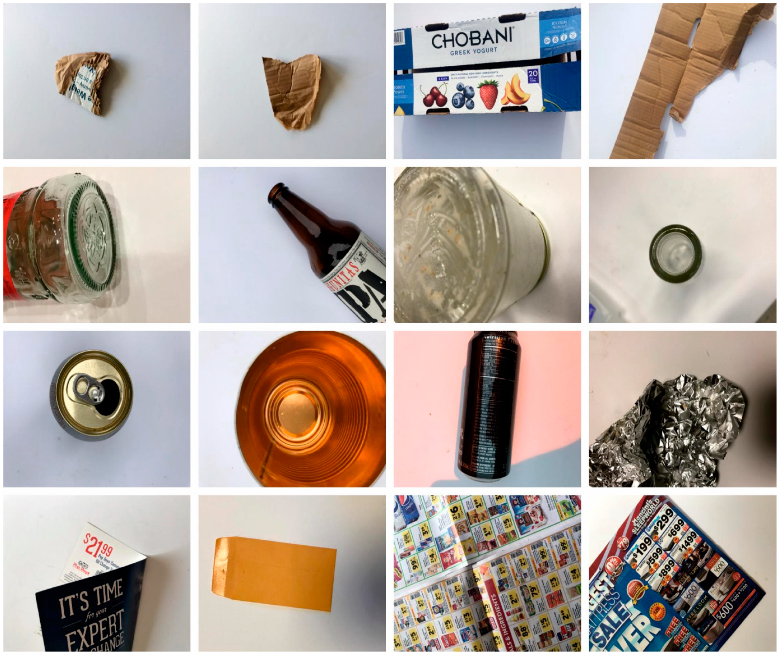
The proposed model is simulated using the Python 3.6.5 tool on PC i5-8600k, GeForce 1050Ti 4GB, 16GB RAM, 250GB SSD, and 1TB HDD. The experimental validation of the AEOIDL-SWM model is tested by means of the garbage classification dataset from the Kaggle repository [
23]. The dataset holds 2467 samples, with six classes, as illustrated in
Table 1. A few sample images are displayed in
Figure 3.
Figure 4 represents three confusion matrices provided through the AEOIDL-SWM model for the applied data. The figure shows that the AEOIDL-SWM model has the capability of recognizing all six waste class labels.
Table 2 demonstrates brief waste classification results of the AEOIDL-SWM method.
Figure 5 examines the waste classification results of the AEOIDL-SWM system on the entire dataset. The AEOIDL-SWM model classified cardboard samples with
of 99.39%,
of 98.71%,
of 97.46%,
of 98.08%,
of 98.61%, and MCC of 97.72%. In addition, the AEOIDL-SWM system categorized metal samples with
of 99.19%,
of 97.03%,
of 98%,
of 97.51%,
of 98.71%, and MCC of 97.03%. Moreover, the AEOIDL-SWM approach categorized trash samples with
of 99.51%,
of 95.28%,
of 95.28%,
of 95.28%,
of 97.51%, and MCC of 95.02%.
Figure 6 shows the waste classification results of the AEOIDL-SWM technique on 70% of the TR dataset. The AEOIDL-SWM system categorized cardboard samples with
of 99.42%,
of 98.54%,
of 97.83%,
of 98.18%,
of 98.78%, and MCC of 97.84%. Furthermore, the AEOIDL-SWM system categorized metal samples with
of 99.25%,
of 97.20%,
of 98.23%,
of 97.72%,
of 98.84%, and MCC of 97.27%. Moreover, the AEOIDL-SWM process categorized trash samples with
of 99.42%,
of 94.38%,
of 94.38%,
of 94.38%,
of 97.04%, and MCC of 94.08%.
Figure 7 reflects the waste classification results of the AEOIDL-SWM method on 30% of the TS dataset. The AEOIDL-SWM system classified cardboard samples with
of 99.33%,
of 99.12%,
of 96.58%,
of 97.84%,
of 98.21%, and MCC of 97.45%. Furthermore, the AEOIDL-SWM system classified metal samples with
of 99.06%,
of 96.61%,
of 97.44%,
of 97.02%,
of 98.40%, and MCC of 96.46%. Moreover, the AEOIDL-SWM technique classified trash samples with
of 99.73%,
of 97.37%,
of 97.37%,
of 97.37%,
of 98.61%, and MCC of 97.23%.
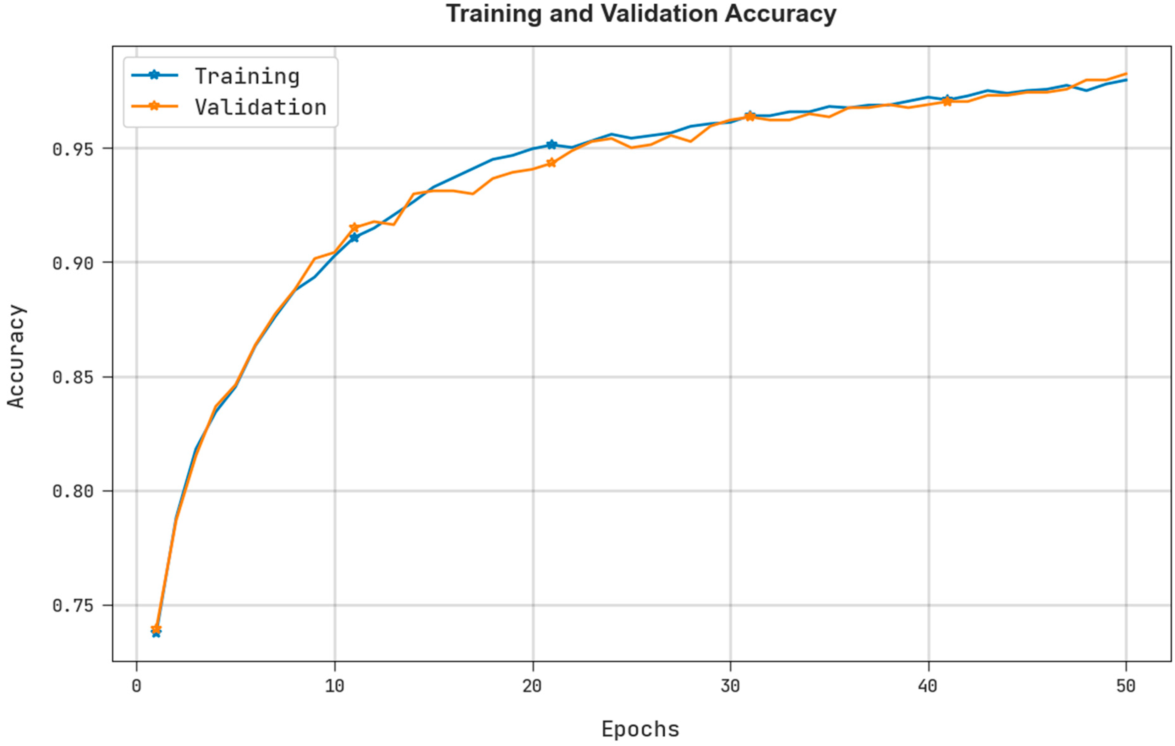
The training accuracy (TRA) and the validation accuracy (VLA) attained using the AEOIDL-SWM system under the test database are shown in
Figure 8. The simulation result show that the AEOIDL-SWM approach attained the highest TRA and VLA. In particular, the VLA appeared to be less than the TRA.
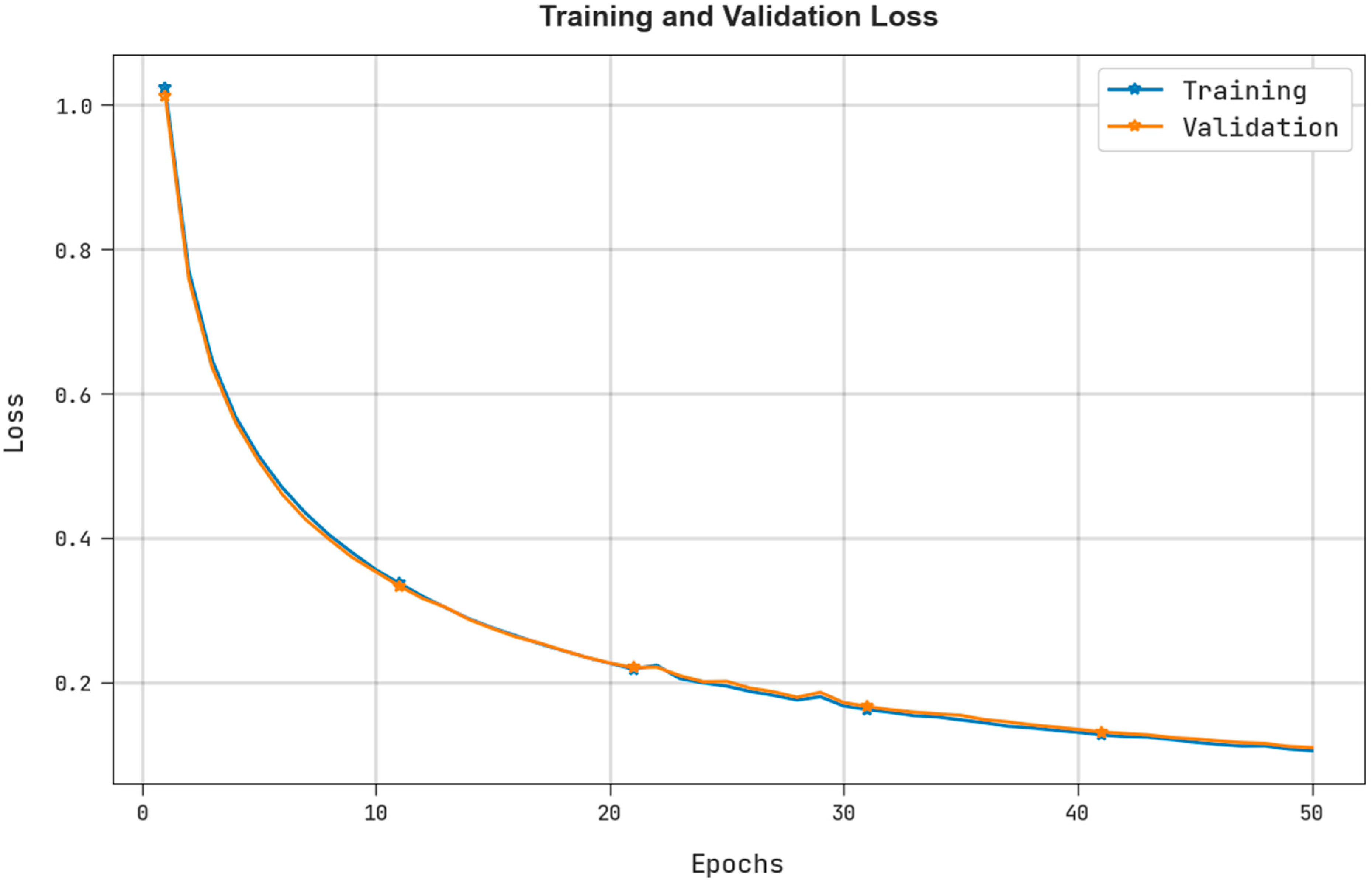
The training loss (TRL) and validation loss (VLL) achieved by the AEOIDL-SWM system under test database are demonstrated in
Figure 9. The simulation outcomes show that the AEOIDL-SWM technique achieved the lowest values of TRL and VLL. Particularly, the VLL is lower than the TRL.
A clear precision recall (PR) examination of the AEOIDL-SWM system under the test database is depicted in
Figure 10. The figure denotes that the AEOIDL-SWM approach resulted in improved PR values under each class.
A brief ROC analysis of the AEOIDL-SWM tactic under the test database is illustrated in
Figure 11. The results indicate that the AEOIDL-SWM method displayed its ability to classify dissimilar categories using the test datasets.
Table 3 depicts a detailed comparative examination of the AEOIDL-SWM approach with other DL algorithms [
15].
Figure 12 illustrates comparative
and
results of the AEOIDL-SWM model over other models. The outcomes point out the enhanced results of the AEOIDL-SWM system. Based on
, the presented AEOIDL-SWM model achieved an improved
of 99.42%, whereas the MLH-CNN, DLSODC-GWM, ResNet50, and VGG16 models obtained a reduced
of 91.94%, 98.73%, 74.31%, 73.12%, and 56.88%, correspondingly. Meanwhile, based on the
, the presented AEOIDL-SWM model has accomplished a better
of 98.10%, while the MLH-CNN, DLSODC-GWM, ResNet50, and VGG16 approaches a exhibited lower
of 91.09%, 96.64%, 71.78%, 67.78%, and 54.69%, correspondingly.
Figure 13 exemplifies a comparative
and
outcome of the AEOIDL-SWM methodology over other techniques. The outcomes described the improved results of the AEOIDL-SWM system. Based on
, the presented AEOIDL-SWM methodology accomplished a better
of 98.16%, while the MLH-CNN, DLSODC-GWM, ResNet50, and VGG16 methods attained reduced
of 90.73%, 95%, 71.36%, 68.83%, and 52.14%, correspondingly. Meanwhile, based on
, the presented AEOIDL-SWM methodology achieved an improved
of 98.06%, whereas the MLH-CNN, DLSODC-GWM, ResNet50, and VGG16 techniques have showed lower
of 91.42%, 92.24%, 72.41%, 68.29%, and 59.31%, correspondingly. These results assure the supremacy of the presented AEOIDL-SWM model over other DL models.


