Evaluating the Impact of Dynamic Changes in Grasslands on the Critical Ecosystem Service Value of Yanchi County in China from 2000 to 2015

Abstract

Grasslands are the basis for sustainable development in the northern farming-pastoral transition zone of China, with functions of human production, living, and ecology. Large-scale human activities inevitably lead to significant changes in grasslands, resulting in significant impacts on ecosystem services. To this end, we quantitatively estimated the ecosystem services value in each positive succession process (the improvement in the coverage or area of grasslands) and negative succession process (the degradation in the coverage or area of grasslands). The results indicated that (1) grasslands showed an improving trend from 2000 to 2015. The grassland improvement from low to high coverage dominated the positive succession process. Grassland degradation from high to low coverage dominated the negative succession process. (2) The total ecosystem services value increased by 25,294.87 × 10⁴ yuan from 2000 to 2015. The grassland improvement from low to high coverage was the most important process that led to the increase in ecosystem service value. The degradation between grasslands and non-grasslands was the key process that led to the decrement in ecosystem services value. (3) The impact of grassland dynamics on the regional ecosystem service value showed significant spatial heterogeneity at the town scale. The results will provide some implications for the sustainable development of grassland ecosystem services to improve human well-being.

1. Introduction

Ecosystem services (ESs) are benefits obtained directly or indirectly through ecosystem functions [1], which are directly linked to human well-being. As one of the most important ecosystem types on the planet, grasslands are not only an important production base for animal husbandry, but they also provide multiple ESs, including climate regulation, water conservation, preventing wind erosion and stabilizing sands, and maintaining biodiversity [2], which play an important role in ensuring ecological security [3]. With population growth, economic development, and rapid urban expansion, large-scale human activities inevitably lead to significant changes in grasslands, which seriously affect the structure and function of grassland ecosystems, leading to a significant alteration in regional ESs [4,5]. For example, the species richness and vegetation coverage (VC) increased during the positive succession of grasslands, which may lead to the improvement of ESs. The research by Sawut et al. [6] found that the increasing areas of high coverage grasslands led to the improvement of ESs in the Ugan-Kuqa River Delta Oasis of China from 2000 to 2008. Thus, identifying the impact of dynamic changes in grasslands on ESs is an effective approach to the sustainable management of grassland resources and improving human well-being.

The assessment of the ecosystem services value (ESV) is an effective method to analyze the impact of land use change on regional ESs. The ESV can be valued in either monetary or nonmonetary units [7]. Specifically, the ESV in monetary units can be directly incorporated into resource and environmental management. Recently, several methods have been used to estimate the monetary values of ESs, such as the value equivalent method and model calculation method [8]. In 1997, Costanza et al. [1] calculated the global ESV of US $33 × 10¹² per year based on the value equivalent method, which was an important attempt to comprehensively evaluate the ESV of grasslands. Subsequently, the equivalent factor proposed by Costanza was modified with remote sensing data to estimate the ESV. However, the disadvantage of this approach is that it ignores the spatial heterogeneity of ES, leading to large uncertainties in ESV [9,10]. With the rapid development of GIS and RS, model calculation methods, such as the ARIES (artificial intelligence for ESs), SolVES (social values for ESs) and InVEST (integrated valuation of ESs and tradeoffs) models have played an increasingly important role in the valuation of ESV [11,12]. In particular, InVEST is a spatially explicit model consisting of multiple modules and can better describe the biophysical processes of ESs, which shows the potential advantages of evaluating ESs [13,14]. Currently, it has been widely used in soil conservation [15], carbon storage [16,17], biodiversity [18,19], and water conservation [20]. In recent years, a large number of studies have been conducted to assess the impact of land use change on ESV. For instance, Ye et al. [21] evaluated the impact of land use change on ESV in Guangzhou and Foshan from 1990 to 2010 using the value equivalent method and found that over one-quarter of land use changed and that the ESV declined by 4.4% (US $201.5 million). Tan et al. [22] studied the relationship between land use change and ESV in the Zhangye Oasis from 1980 to 2015 based on the value equivalent method and found that land use and ESV changed dramatically. These studies have contributed to evaluating the impact of land use on ESV and environmental management. However, it was found that the value equivalent method was mainly used to evaluate ESV, and there is a lack of in-depth quantitative assessments of the impact of grassland dynamics on ESV, which might impede reasonability in the management of grassland resources and the sustainable development of ESs.

Yanchi County is located in the core area of the farming-pastoral transition zone in northern China, and grasslands are the main land use type, accounting for more than 60% of the total area. With the continuous growth of the population and economy, intensive human activities, such as overgrazing, slopeland reclamation, and urban construction, coupled with the serious shortage of water resources, has resulted in a series of ecological problems, such as vegetation degradation and land desertification. To solve ecological problems, ecological projects, such as the Grain for Green program and afforestation, have been implemented. Yanchi took the lead in implementing the grazing prohibition policy for the whole county in November 2002, which provided a habitat for the recovery of grassland vegetation [23]. The human activities mentioned above inevitably lead to significant changes in land use, resulting in significant impacts on the monetary values of ESs provided by various land uses. Therefore, it is important to identify the impact of dynamic changes in grasslands on the ESV in Yanchi County. To this end, we attempted to break down and quantify the dynamic change in grasslands, estimate the multiple ESs from the biophysical perspective and then evaluate the monetary value of grassland ESs, which will provide some implications for scientific management.

2. Materials and Methods

2.1. Study Area

Yanchi County (106°30′ E~107°41′ E, 37°04′ N~38°10′ N) of the Ningxia Hui Autonomous Region is located in Northwest China (Figure 1), with a total area of 8661 km². It has a typical mild and continental climate with average annual rainfall of 296~355 mm and annual evaporation of 2095~2180 mm [24,25]. There is a shortage of water resources, and historically, groundwater and surface water are completely dependent on rainfall recharge. In addition, according to the remote sensing monitoring dataset for land use provided by the Data Center for Resources and Environmental Sciences, Chinese Academy of Sciences (RESDC) [26], grasslands, including desert grasslands and steppe, accounted for approximately 60%, and croplands and forests accounted for 17% and 13%, respectively. Otherwise, the areas of other land use types, such as water bodies, building land, and unused land, are all small, accounting for approximately 10% of the total. Over the past few decades, the increasing intensity of human activities has inevitably led to significant changes in land use, which poses challenges to the sustainable development of grassland ESs.

2.2. Data Sources

Most of the data used to evaluate the ESV are self-explanatory and are shown in

Table A1. Acquisition and preprocessing of the parameters.

Data	Purpose	Source	Type	Time	Resolution Resolution	References
Annual precipitation	Water yield model input	Calculated with ANUSPLIN and validated by cross-validation, with an RMSE of 16.79 mm	Raster	2000, 2015	30 m	[60,61,62]
Plant evapotranspiration coefficient	Water yield model input	Estimated based on leaf area index	Constant	2000, 2015	--	[63]
Reference evapotranspiration	Water yield model input	Calculated using the Penman–Monteith model	Raster	2000, 2015	30 m	[64]
Seasonality factor	Water yield model input	Obtained by comparing the simulated yield with runoff	Constant	2015	--	[65]
Root restricting layer depth	Water yield model input	A Chinese dataset of soil properties for land surface modelling	Raster	2013	1 km	[66]
Root depth	Water yield model input	Obtained from a relevant study	Constant	2015	--	[66]
Plant available water capacity	Water yield model input	Calculated based on soil texture	Raster	2013	1 km	[67]
Velocity coefficient	Water conservation model input	Obtained according to a relevant study	Constant	2015	--	[68]
Soil saturated hydraulic conductivity	Water conservation model input	Calculated by SPAW software	Raster	2013	1 km	[66]
Market price of freshwater	ESV of water conservation	Groundwater trading in the China water rights exchange	Constant	2000, 2015	--	[69]
Soil carbon	Carbon storage model input	A Chinese dataset of soil properties for land surface modelling	Raster	2013	1 km	[66]
Carbon market price	ESV of carbon storage	Obtained from the China carbon emission trading center	Constant	2015	--	[70]
Rainfall erosivity	Sediment retention model input	Obtained from the relationships with precipitation	Raster	2000, 2015	30 m	[71]
Soil erodibility	Sediment retention model input	Obtained using the EPIC model	Raster	2013	1 km	[72]
Cover management factor	Sediment retention model input	Obtained from a relevant study	Constant	2015	--	[73]
Support practice factor	Sediment retention model input	Obtained according to a relevant study	Constant	2015	--	[74]
Market prices of nutrient N, P and K	ESV of sediment retention	Obtained from the China fertilizer network	Constant	2000, 2015	--	[75]
Percentages of nutrient N, P and K	ESV of sediment retention	A Chinese dataset of soil properties for land surface modelling	Raster	2013	1 km	[66]
Normalized vegetation index	Vegetation coverage of grasslands	Obtained through band math in ENVI 5.2	Raster	2000, 2015	30 m	[76]

Notes: -- is used to denote the lack of spatial resolution for data of constant type.

, but a few data, such as land use and vegetation carbon, require more introduction. All the data used to evaluate the ESs from the biophysical perspective were resampled at a spatial resolution of 30 m and projected using the Krasovsky_1940_Albers coordinate system.

We produced a new land use map suitable for analyzing grassland dynamics. A large-scale remote sensing monitoring dataset for land use [26] is available for Yanchi County. However, only three types of grasslands, including high coverage, medium coverage, and low coverage grasslands, were considered, so an exhaustive assessment of dynamic change in grasslands with different coverages could not be performed. To this end, we implemented the following five aspects to produce a new land use map suitable for analyzing grassland dynamics: (1) The field measurement of grassland VC was carried out from August 19 to August 30 in 2015, and we attained a total of 63 sample sites of grasslands with a size of 30 m × 30 m and 315 grassland plots of 1 m × 1 m with the five-point sampling method (Figure 1) [27,28]. Thus, the digital camera photography method, which has the advantages of relative economy, efficiency, and more accurate results, was used to measure the VC of grasslands [29,30]. (2) We randomly selected 70% of the measured grassland VC data, and regression analysis was used to construct the model of grassland VC with the normalized difference vegetation index (NDVI). (3) Taking the randomly selected 30% of measured VC data as the “truth value”, the root mean square error (RMSE) between two data was calculated. A comprehensive comparison of R² and RMSE of all regression models showed that the R² of linear regression model VC = 142.47NDVI + 4.02 was the highest (R² = 0.90), while the RMSE (7.67) was the lowest of all the other models. Therefore, based on the grassland boundary obtained from the remote sensing monitoring dataset for land use [26], the linear regression model VC = 142.47NDVI + 4.02 was used to estimate the VC of grasslands in 2000 and 2015. (4) Based on the grassland classification standards provided by the code of practice for grassland resource surveys [31], we classified them into five types: low coverage grasslands (0~20%), medium-low coverage grasslands (20~40%), medium coverage grasslands (40~60%), medium-high coverage grasslands (60~80%) and high coverage grasslands (80~100%). (5) Non-grasslands, including cropland, forest, water body, building land, and unused land, were still obtained from the remote sensing monitoring dataset for land use [26].

Vegetation carbon is one of the important data used to evaluate carbon storage. We have implemented the following five aspects to evaluate the vegetation carbon: (1) we sampled the aboveground parts of different species of grassland vegetation and recorded the fresh weight of biomass in the field measurement of grassland vegetation. (2) The dry weight of grasslands in the aboveground parts was measured by drying the aboveground biomass from the sample sites in a laboratory drying oven (drying at a constant 65 °C until the mass was constant). Then, the aboveground carbon storage of grasslands was obtained by multiplying the dry weight of grasslands in the aboveground parts by the 0.45 coefficient [32,33]. (3) Based on the measured aboveground vegetation carbon (AVC) of grasslands and the NDVI, a linear regression model of AVC = 376.95NDVI−28.20 (R² = 0.84) was used to simulate the AVC of grasslands in Yanchi County. (4) We determined the total vegetation carbon of grasslands based on the relationship that the aboveground carbon storage of grasslands accounts for 23.48% of the total vegetation carbon of grasslands provided by Cheng et al. [33]. (5) The vegetation carbon of the forest was obtained according to the relevant study provided by Bao. [34] and Zhang et al. [35], while the vegetation carbon of cropland was referenced from the relevant studies of Han et al. [36] and Tuo et al. [37].

2.3. Methods

2.3.1. Ecosystem Services Valuation

Combined with the regional characteristics of grasslands in Yanchi County, three key ES types, including water conservation, carbon storage, and sediment retention, were selected based on the Millennium Ecosystem Assessment (MEA) [38]. First, we estimated multiple ESs from a biophysical perspective based on the InVEST, and then, the market value method was used to estimate the monetary value of ESs.

Water Conservation

(1)

The amount of water conservation

Water conservation is calculated in two steps. In the first step, the water yield is calculated based on the Budyko curve and annual average precipitation [39,40]. Based on the water balance principle, the annual water yield is defined as the difference between rainfall and evapotranspiration. The formula of annual water yield (Yield) is given as follows:

$$Yield=\left(1-\frac{AET}{P}\right)\times P$$

(1)

where AET is the annual actual evapotranspiration (mm), and P is the annual precipitation (mm). AET/P denotes the evapotranspiration portion of the water balance and is calculated by using the approximation of the Budyko curve developed by Fu [41] and Zhang et al. [42]:

$$\frac{AET}{P}=1+\frac{PET}{P}-{\left[1+{\left(\frac{PET}{P}\right)}^{\omega }\right]}^{\raisebox{1ex}{$1$}\!\left/ \!\raisebox{-1ex}{$\omega $}\right.}$$

(2)

where PET is the potential evapotranspiration calculated with Formula (3). ω is a nonphysical parameter that characterizes the natural climatic-soil properties [42] and is calculated as shown in Formula (4):

$$PET=K_c\left(l\right)\times E{T}_0$$

(3)

$$\omega =Z\frac{Min\left(Rest.layer.depth,root.depth\right)\times PAWC}{P}+1.25$$

(4)

where $K_c\left(l\right)$ denotes the plant evapotranspiration coefficient. $E{T}_0$ is the reference evapotranspiration (mm/d). Z is a seasonality factor that presents the seasonal rainfall distribution and rainfall depths [43,44]. $Rest.layer.depth$ is the root restricting layer depth (mm). $root.depth$ is the root depth (mm). PAWC is the plant’s available water capacity.

In the second step, the amount of water conservation is calculated by water conservation factors, such as the topographic index, soil saturated hydraulic conductivity, and velocity coefficient. The formula for water conservation (Retention) is provided as follows:

$$Retention=Min\left(1, \frac{249}{Velocity}\right)\times Min\left(1,\frac{0.9\times TI}{3}\right)\times Min\left(1,\frac{Ksat}{300}\right)\times Yield$$

(5)

where Retention is the water conservation (mm). Velocity is the velocity coefficient. Ksat is the soil saturated hydraulic conductivity (cm/d). TI is a topographic index, which can be calculated using Formula (6):

$$TI=\log \left(\frac{Drainage\_Area}{Soil depth\times PercentSlope}\right)$$

(6)

where Drainage_Area is the number of catchment grids (m²). The PercentSlope is the percentage of the slope.

(2)

The monetary value of water conservation

The formula is given as follows:

$$WC=Retention\times D$$

(7)

where WC is the monetary value of water conservation (yuan). Retention is the amount of water conservation (mm). D is the market price of freshwater (yuan/ton).

Carbon Storage

(1)

The amount of carbon storage

Carbon storage includes vegetation carbon and soil carbon. The formula is given as follows:

$$C_v=C_{veg}+C_{soil}$$

(8)

where $C_v$ is the amount of carbon storage (ton/ha) and $C_{veg}$ is the amount of vegetation carbon (ton/ha). $C_{soil }$ denotes the amount of soil carbon (ton/ha).

(2)

The monetary value of carbon storage

The formula is given as follows:

$$CS=C_v\times \frac{S}{0.2727}$$

(9)

where CS is the monetary value of carbon storage (yuan). $C_v$ is the amount of carbon storage (ton/ha). S is the market price of carbon (yuan/ton), and 0.2727 is the conversion coefficient between carbon and carbon dioxide.

Sediment Retention

(1)

The amount of sediment retention

The total amount of sediment retention was calculated by estimating how much sediment was retained based on the sediment delivery ratio across the basin. The calculation is divided into 2 steps. In the first step, the revised universal soil loss equation [45,46] is used to calculate the actual soil loss (usle) considering anthropogenic influences, such as management and engineering measures. The calculation is given as follows:

usle = R × K × LS × P × C

(10)

where R is the rainfall erosivity (MJ·mm/(hm²·h)). K is the soil erodibility factor (t·hm²·h/(hm²·MJ·mm)). LS is the slope length-gradient factor. C is the cover management factor. P is the support practice factor.

In the second step, the sediment delivery ratio (SDR) is obtained from the conductivity index $IC$, and the calculation is given as follows:

$$SDR=\frac{SD{R}_{max}}{1+\exp \left(\frac{I{C}_0-IC}{k}\right)}$$

(11)

where $SD{R}_{max}$ is the maximum SDR. $I{C}_0$ and $k$ are calibration parameters. $IC$ is calculated by the following formula:

$$IC={\log }_{10}\left(\frac{D_{up}}{D_{dn}}\right)$$

(12)

where $D_{up}$ is the area upslope. $D_{dn}$ is the flow path between the pixel and the nearest stream.

In summary, the sediment retention in the InVEST model is calculated as follows:

$$E=R\times K\times LS\times \left(1-CP\right)\times SDR$$

(13)

(2)

The monetary value of sediment retention-

The formula is given as follows:

$$SC=E\times N\times T_N+E\times P\times T_P+E\times K\times T_K$$

(14)

where SC is the value of maintenance of soil fertility (yuan). E is the sediment retention (ton). N, P, and K are the percentages (%) of alkali-hydrolyzable nitrogen, available phosphorus, and available potassium in the retained sediment, respectively. $T_N$, $T_P$ and $T_K$ denote the market prices of nitrogen, phosphorus, and potassium, respectively.

2.3.2. Assessing the Impact of the Dynamic Change in Grasslands on the Regional Ecosystem Service Value

In this study, the dynamic change in grasslands refers to positive and negative succession. The positive succession of grasslands included positive succession between grasslands with different coverage (such as grasslands with low coverage improved to grasslands with medium coverage) and positive succession between grasslands and non-grasslands (such as unused land that transitioned to grasslands). The negative succession of grasslands included negative succession between grasslands with different coverage (such as grasslands with medium coverage degraded to grasslands with low coverage) and negative succession between grasslands and non-grasslands (such as grasslands degraded to farmland). The impact of grassland dynamics on the regional ESV was assessed by decomposing the process of grassland dynamics and the change in the other land uses, which can be obtained from the following formulas.

$$ES{V}_v=ES{V}_{id}+ES{V}_{dd}+ES{V}_{ig}+ES{V}_{dg}$$

(15)

$$ES{V}_{id}=ES{V}_{id\_1}+ES{V}_{id\_2}$$

(16)

$$ES{V}_{ig}=ES{V}_{ig\_1}+ES{V}_{ig\_2}$$

(17)

where $ES{V}_v$ is the change in the ESV. $ES{V}_{id}$ refers to the increase in ESV generated by the transition between grasslands and non-grasslands. $ES{V}_{dd}$ refers to the decrease in ESV produced by the degradation between grasslands and non-grasslands (this value is negative). $ES{V}_{ig}$ refers to the increase in ESV produced by the change between grasslands with different coverages. $ES{V}_{dg}$ refers to the decrease in ESV caused by the transition between grasslands with different coverages (this value is also negative). $ES{V}_{id\_1}$ refers to the increase in ESV caused by the transition between grasslands and non-grasslands in the ES increase-ESV increase type of ESs. $ES{V}_{id\_2}$ refers to the increase in ESV caused by the transition between grasslands and non-grasslands in the ES decrease-ESV increase type of ESs. $ES{V}_{ig\_1}$ refers to the increase in ESV caused by the transition between grasslands with different coverages in the ES increase-ESV increase type of ESs; $ES{V}_{ig\_2}$ refers to the increase in ESV caused by the transition between grasslands with different coverages in the ES decrease-ESV increase type of ESs.

3. Results

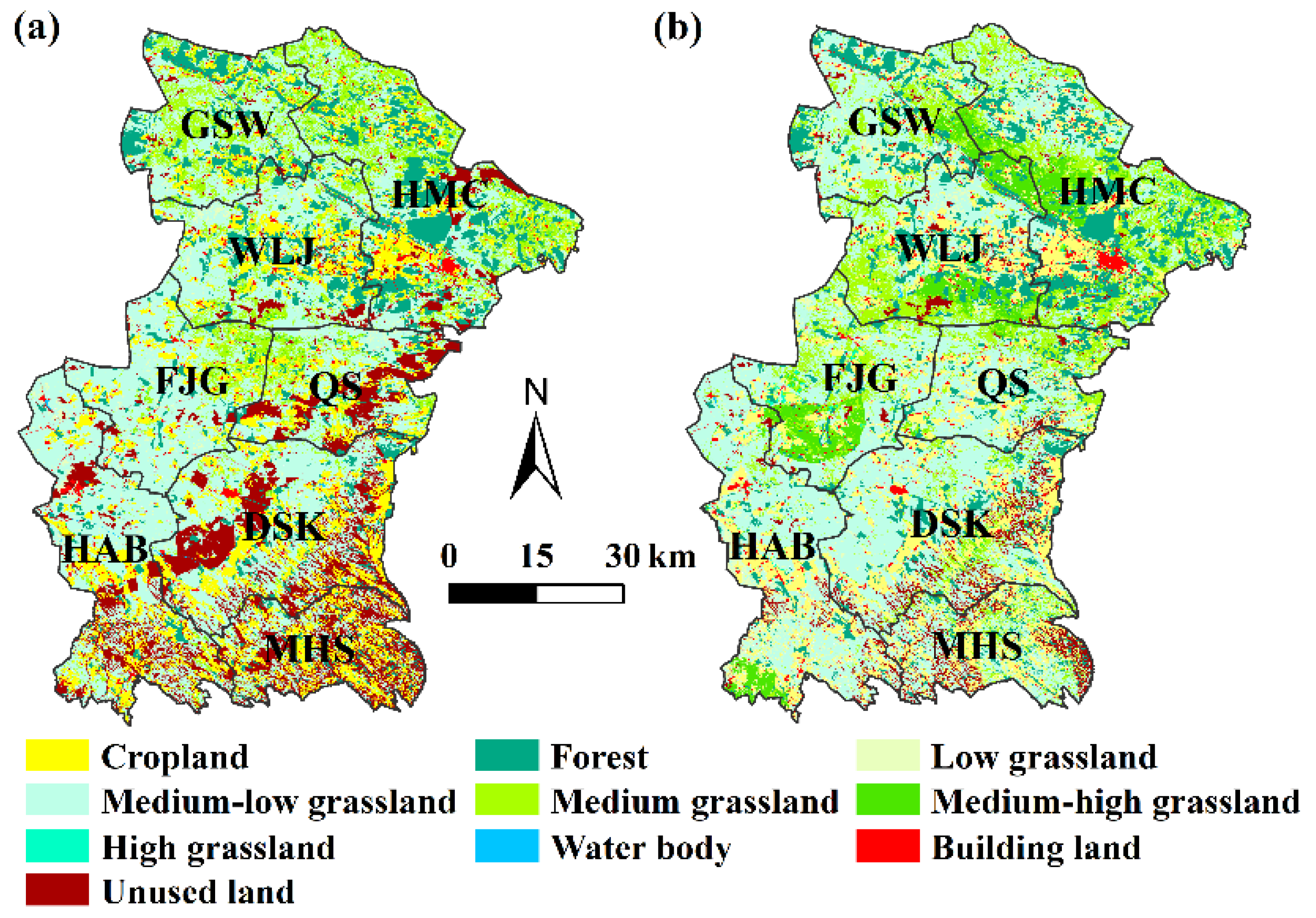
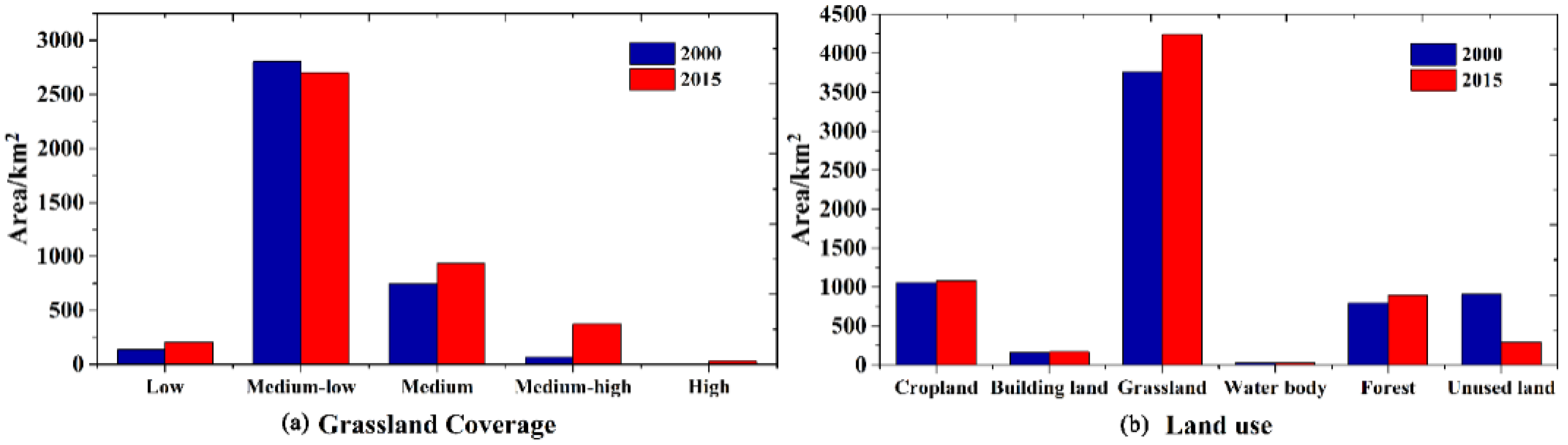
3.1. Dynamic Change in Grasslands from 2000 to 2015

In 2000, the land use in Yanchi County was dominated by grasslands with medium-low coverage (Figure 2a). Additionally, the unused land was mainly distributed in Dashuikeng, Huianbao, Qingshan, and Mahuangshan, and its area was slightly larger than that of forests. However, the area of unused land significantly decreased in 2015 (Figure 2b). Among them, a large amount of unused land was converted to forest and grasslands with medium and medium-high coverage, resulting in an overall improving trend in the areas of medium and medium-high coverage grasslands and forests from 2000 to 2015.

There was a significant difference in the area of grasslands with different coverages and non-grasslands, and grassland coverage showed an overall improving trend from 2000 to 2015 (Figure 3a,b). The areas of grasslands with high, medium-high, medium, and low coverage all increased, especially the area of grasslands with medium-high coverage, which increased significantly from 66.23 km² to 371.61 km² over the past 15 years. However, the area of grasslands with medium-low coverage decreased from 2804.86 km² to 2698.73 km².

According to the statistical results of the grassland dynamics in the towns (

Table 1. The area (km²) and percentage (%) of regions that experienced positive succession and negative succession of grasslands.

	Positive Succession				Negative Succession
	Positive Succession 1		Positive Succession 2		Negative Succession 1		Negative Succession 2
	Area (km2)	Percentage	Area (km2)	Percentage	Area (km2)	Percentage	Area (km2)	Percentage
DSK	67.89	1.01	186.44	2.79	29.17	0.44	1.80	0.03
QS	67.22	1.00	108.57	1.62	49.61	0.74	0.17	0
FJG	194.39	2.91	14.33	0.21	65.53	0.98	3.66	0.05
HMC	224.61	3.36	65.14	0.97	130.12	1.94	35.95	0.54
WLJ	214.44	3.20	20.21	0.30	53.01	0.79	0.93	0.01
GSW	92.64	1.38	5.42	0.08	136.46	2.04	0.78	0.01
MHS	17.95	0.27	144.91	2.16	11.93	0.18	0.28	0
HAB	79.07	1.18	109.06	1.63	70.86	1.06	2.47	0.04
Yanchi	958.21	14.32	654.08	9.78	546.96	8.17	46.04	0.69

Notes: Positive succession 1 indicates that grasslands improved from low coverage to high coverage; positive succession 2 indicates the improvement between grasslands and non-grasslands. Negative succession 1 means that grasslands degraded from high coverage to low coverage. Negative succession 2 indicates degradation between grasslands and non-grasslands. The percentage represents the ratio of negative succession/positive succession 1 and 2 to the total area of grasslands in 2015.

), the total area of regions that experienced positive succession among different grasslands was 958.21 km² (Table 1). This region was mainly distributed in Huamachi, Fengjigou, and Wanglejing (Figure 4a). In addition, the area of positive succession between grasslands and non-grasslands was 654.08 km². The smallest area was in Gaoshawo, with only 5.42 km², while the largest area was in Dashikeng, with 186.44 km² (Figure 4a). However, the area of grasslands with high coverage that degraded to grasslands with low coverage was 546.96 km², and this region was mainly distributed in Gaoshawo and Huamachi (Figure 4b). Moreover, the area of negative succession between grasslands and non-grasslands was only 46.04 km² in the whole county. The largest area that experienced this succession was Huamachi town (35.95 km²), and the areas in other towns were less than 4 km².

In conclusion, the areas of regions that experienced positive and negative succession accounted for 24.10% and 8.86% of the total area in the county, respectively, indicating that grasslands have shown an overall improving trend over the past 15 years. Specifically, the land that experienced positive succession between grasslands with different coverages and between grasslands and non-grasslands accounted for 14.32% and 9.78%, respectively. Grassland degradation from high coverage to low coverage dominated the negative succession process, which accounted for 8.17% of the whole area in the county.

3.2. Impact of the Dynamic Change in Grasslands on the Regional ESs and ESV

The total ESs of the whole county increased by 976.25 × 10⁴ tons from 2000 to 2015 (

Table 2. The change in ESs (10⁴ tons) induced by grassland and non-grassland changes.

	$\mathit{E}{\mathit{S}}_{\mathit{i}\mathit{d}}$	$\mathit{E}{\mathit{S}}_{\mathit{d}\mathit{d}}$		$\mathit{E}{\mathit{S}}_{\mathit{i}\mathit{g}}$	$\mathit{E}{\mathit{S}}_{\mathit{d}\mathit{g}}$
		$\mathit{E}{\mathit{S}}_{\mathit{d}\mathit{d}\_1}$	$\mathit{E}{\mathit{S}}_{\mathit{d}\mathit{d}\_2}$		$\mathit{E}{\mathit{S}}_{\mathit{d}\mathit{g}\_1}$	$\mathit{E}{\mathit{S}}_{\mathit{d}\mathit{g}\_2}$
DSK	58.56	−0.74	−73.53	79.20	−0.02	−0.11
QS	17.81	−0.20	−18.76	51.80	0	−0.04
FJG	2.68	−0.03	−2.24	51.48	−0.01	−0.02
HMC	43.63	0	−0.32	220.00	0	−0.01
WLJ	4.58	−0.01	−0.74	101.54	0	−0.01
GSW	1.22	0	0	72.76	0	0
MHS	190.72	−1.14	−43.05	30.35	−0.03	−0.23
HAB	26.34	−1.88	−49.80	23.56	−0.07	−0.92
Yanchi	345.55	−4.01	−188.44	630.70	−0.13	−1.34

), the increment of the ESs was caused by the positive succession between grasslands with different coverages ($E{S}_{ig}$) reached 630.70 × 10⁴ tons, and the contribution to the ES increment was 64.60%. The increase in ESs is caused by the improvement between grasslands and non-grasslands ($E{S}_{id}$) was 345.55 × 10⁴ tons, and the contribution to the ES increase was 35.40%. Negative succession between grassland dynamics decreased by 193.92 × 10⁴ tons and the decreases in ESs produced by the degradation between grasslands and non-grasslands ($E{S}_{dd\_2}$) accounted for 99.24% of the total decrement.

The total ESV of the whole county increased by 25,294.87 × 10⁴ yuan from 2000 to 2015, which is mainly attributed to the positive succession between grasslands with different coverages and between grasslands and non-grasslands (

Table 3. The regional ESV (10⁴ yuan) change induced by grassland and other land use changes.

	$\mathit{E}\mathit{S}{\mathit{V}}_{\mathit{i}\mathit{d}}$		$\mathit{E}\mathit{S}{\mathit{V}}_{\mathit{d}\mathit{d}}$	$\mathit{E}\mathit{S}{\mathit{V}}_{\mathit{i}\mathit{g}}$		$\mathit{E}\mathit{S}{\mathit{V}}_{\mathit{d}\mathit{g}}$
	$\mathit{E}\mathit{S}{\mathit{V}}_{\mathit{i}\mathit{d}\_1}$	$\mathit{E}\mathit{S}{\mathit{V}}_{\mathit{i}\mathit{d}\_2}$		$\mathit{E}\mathit{S}{\mathit{V}}_{\mathit{i}\mathit{g}\_1}$	$\mathit{E}\mathit{S}{\mathit{V}}_{\mathit{i}\mathit{g}\_2}$
DSK	2212.49	12.14	−18.51	1447.84	0	−1.81
QS	1046.92	6.03	−11.65	1129.07	0	−2.65
FJG	115.57	1.67	−9.24	2604.44	0.01	−3.53
HMC	821.54	3.04	−45.20	3590.05	0.04	−10.09
WLJ	166.44	1.22	−12.67	2821.75	0.01	−4.57
GSW	9.77	0.24	−8.16	1715.45	0.03	−5.26
MHS	4065.53	17.37	−7.25	585.55	0	−0.71
HAB	1556.74	27.70	−6.60	1336.22	0	−2.82
Yanchi	9995.00	69.41	−119.27	15,230.37	0.09	−31.44

). The increment of the ESV is caused by the positive succession between grasslands with different coverages ($ES{V}_{ig\_1}$) reached 15,230.37 × 10⁴ yuan, and the contribution to the ESV increment was 60.21%. In particular, the conversion of medium-low and medium grasslands to higher coverage grasslands played an important role in this value (

Table 4. The impacts of dynamic changes in grasslands on ESV (10⁴ yuan).

	$\mathit{E}\mathit{S}{\mathit{V}}_{\mathit{i}\mathit{d}\_1}$				$\mathit{E}\mathit{S}{\mathit{V}}_{\mathit{i}\mathit{g}\_1}$	$\mathit{E}\mathit{S}{\mathit{V}}_{\mathit{i}\mathit{d}\_2}$				$\mathit{E}\mathit{S}{\mathit{V}}_{\mathit{i}\mathit{g}\_2}$	$\mathit{E}\mathit{S}{\mathit{V}}_{\mathit{d}\mathit{d}}$				$\mathit{E}\mathit{S}{\mathit{V}}_{\mathit{d}\mathit{g}}$
	Farmland	Forest	Water Area	GRASS Land	Grass Land	Farmland	Forest	Water Area	Grass Land	Grass Land	Farmland	Forest	Water Area	Grass Land	Grass Land
low	89.15	598.15	0.01	--	934.67	0	0.06	0.01	--	0	−1.32	−1.82	0	--	−2.35
medium-low	262.0	5247.9	0	--	10,450.0	0.03	0.64	0	--	0.04	−8.67	−55.67	−0.02	--	−10.37
medium	43.01	546.74	0.01	--	3353.53	0	0.23	0	--	0.05	−4.66	−39.66	−0.09	--	−11.66
medium-high	6.03	54.95	0	--	360.78	0.01	0.02	0.02	--	0	−1.14	−6.86	−0.12	--	−3.16
high	1.00	12.25	0	--	30.94	0	0.01	0	--	0	−0.05	−2.84	0	--	−0.58
farmland	--	--	--	298.0	--	--	--	--	2.14	--	--	--	--	0	--
forest	--	--	--	442.8	--	--	--	--	0.79	--	--	--	--	−0.03	--
water area	--	--	--	39.03	--	--	--	--	0.46	--	--	--	--	0	--

). The increase in the ESV was caused by the improvement between grasslands and non-grasslands ($ES{V}_{id\_1}$) was 9995 × 10⁴ yuan, and the contribution to the ESV increase was 39.52%. In particular, the conversion of grasslands to forests played an important role in this value (Table 4). Negative succession between grassland dynamics decreased by 150.71 × 10⁴ yuan and the decreases in ESV were produced by the transition between grasslands and non-grasslands ($ES{V}_{dd}$) accounted for 79.13% of the total decrement. However, the decrement was smaller than the increment caused by grassland dynamics.

The impact of grassland dynamics on the regional ESV showed significant spatial heterogeneity at the town scale (Table 3 and Figure 5). The towns with an increasing ESV are caused by the positive succession between different grasslands ($ES{V}_{ig\_1}$) were mainly distributed in Gaoshawo, Wanglejing, Huamachi, and Fengjigou, and the contribution to ESV change in the whole county was 59.85%. The towns with an increase in ESV were caused by the improvement between grasslands and non-grasslands ($ES{V}_{id\_1}$) from 2000 to 2015 were mainly distributed in Dashuikeng and Mahuangshan, and the contribution to ESV change in the whole county was 39.28%. In addition, the towns that had a decreasing ESV from 2000 to 2015 were mainly located in Huamachi and Dashuikeng, the transition between grasslands and non-grasslands dominated the regional ESV decrement, and the contribution to ESV change in the whole county was 0.47%.

4. Discussion

The dynamic change in grasslands in Yanchi County was dominated by the positive succession between grasslands with different coverages and between grasslands and non-grasslands, which accounted for 14.32% and 9.78% of the total area of the county, respectively. The area of negative succession accounted for 8.17% of the total area of the county. Overall, grasslands showed a significant trend of improvement; this trend matches the results found in previous studies by Wang [47] and Zhong et al. [48]. Impacted by both climate change and human activities, grasslands have changed dramatically over the past 15 years. A study by Li et al. [49] indicated that the positive succession process is strongly related to natural conditions, such as precipitation, and ecological projects, such as the Grain for Green Project, grazing prohibition, and afforestation. The positive succession of grasslands played a major role in the ESV increment of the whole county. The grassland improvement from low to high coverage was the most important process that led to the regional ESV increase. According to the monitoring results shown in Table 1 and Table 3, the total area of regions that experienced positive succession was 1612.29 km² over the past 15 years, which led to a significant increase in the total ESV of 25,294.87 × 10⁴ yuan. The total area of regions that experienced positive succession among different grasslands was 958.21 km², and the contribution to ESV increase was 60.21%. According to the research conducted by Wang [47], the total ESV of Yanchi County increased from 2002 to 2014, which was mainly attributed to the implementation of grazing prohibition.

Yanchi County is famous for being “the hometown of beach sheep in China”. Intensive human activities, such as illegal grazing and rapid urbanization, destroy vegetation and soil, especially in ecologically fragile regions, which leads to the continued degradation of grasslands and a decline in ESV. Table 1 and Table 3 show that the negative succession between grasslands with different coverages accounted for 8.17% of the total area, and the contribution to ESV decrement was 20.87%, while the negative succession between grasslands and non-grasslands only accounted for 0.69% of the total area, and the contribution to ESV decrement was 79.13%. This result indicates that the degradation between grasslands and non-grasslands was the key process that led to the ESV decrement in Yanchi County. This region was mainly distributed in Huamachi. The resulting values in this region might be attributed to intensive human activities. Among the 8 towns in the whole county, Huamachi has the largest population and the most developed economy, with a serious shortage of water resources. According to statistical data, the population in Huamachi experienced an obvious increase from 44,762 persons in 2003 to 57,527 persons in 2015 [50]. With the continuous growth of the population and economy, the increasing intensity of human activities poses new challenges to the utilization of water resources. These are important factors that place pressure on the local ESV.

Although Yanchi County, located in a farming-pastoral transition zone, focuses on animal husbandry, cropland is the second largest type of land use, accounting for 17% of the total area of the county, and there are large irrigation regions (such as the Yang Huang irrigation and Kujing irrigation regions). As shown in Table 3, the ESV caused by the conversion from grasslands to cropland increased by a total of 401.23 × 10⁴ yuan, while the increase in ESV induced by the conversion from cropland into grasslands totaled 300.14 × 10⁴ yuan, indicating that cropland played an important ecological role in improving the regional ESV. However, Table 3 also shows that an ESV change was produced by the conversion from grasslands to cropland, with a decrease of 15.84 × 10⁴ yuan, while the ESV decrease in the conversion from cropland to grasslands was almost zero, which implied that the monetary outcomes for cropland had a higher risk than those for grasslands from the standpoint of ESs because there are tradeoffs and synergies among multiple ESs due to the heterogeneity and diversity of ESs and human preferences. When a large supply of food is needed with an increase in population, the neglect of tradeoffs and synergies of ESs leads to an increase in food provisioning ESs at the expense of other ESs, and negative services, such as destruction by erosion and the loss of soil fertility, may occur, translating to a negative contribution to the total ESV [51]. Therefore, land managers should shift from the production of food through agricultural activities, such as sowing and harvesting, to an integrated practice of land development, utilization, and conservation to maximize economic and ecological benefits.

We broke down the processes of grassland dynamics and quantitatively evaluated the ESV change in each process to assess the impact of dynamic changes in grasslands on regional ESV. The results provide some implications for realizing the scientific planning and sustainable development of grassland ESs. However, several deficiencies remain in this study. First, due to data limitations, other ESs, such as wind prevention and sand fixation services of grasslands, have not been considered in the assessment of ESV, although a study provided by Xu et al. [52] found that wind prevention and sand fixation services provided by Yanchi County are of considerable economic value. Second, in the field survey of vegetation carbon storage in grassland, only aboveground vegetation was sampled, not underground vegetation and litter. On this basis, based on the aboveground carbon storage obtained, the total vegetation carbon of grasslands was calculated based on the relationship that the aboveground carbon storage of grasslands accounts for 23.48% of the total vegetation carbon of grasslands [32,33]. However, underground and litter carbon storage limits the assessment accuracy of the overall carbon storage. Thus, it is essential to conduct field surveys of underground and litter carbon storage in future work. Third, the uncertainty in ESV was not considered or quantified in this paper. The parameters used to estimate the ESV are generally obtained through sampling observations or literature. However, due to shifts in preferences or environmental conditions, the values of parameters (such as the carbon dioxide (CO₂) market price) are often subjected to wide swings, deeply affecting the accuracy of ESV and impeding reasonability in environmental management [53,54]. Recently, a few studies have highlighted that there were large uncertainties in the ESV and have proposed that conducting uncertainty analysis (UA) in ESV will increase the credibility of the results [55,56]. Monte Carlo, a stochastic simulation algorithm, can quantify the total ESV once the probability distributions and sample sizes of the parameters are defined, which shows potential advantages in quantifying the uncertainty in ESV [57,58,59]. Therefore, efforts should be made to improve the accuracy of ESV by performing the UA in ESV based on Monte Carlo simulation.

5. Conclusions

To achieve the sustainable development of grassland ESs, we broke down the dynamic change processes of grasslands, estimated the multiple ESs from the biophysical perspective, and then evaluated their ESVs in each succession process. The results are described as follows: (1) Grasslands showed an overall improving trend from 2000 to 2015. (2) The positive succession of grasslands played a major role in the ESV increment of the whole county. Specifically, grassland improvement from low to high coverage was the most important process that led to the regional ESV increase. These regions were mainly distributed in Gaoshawo, Wanglejing, and Fengjigou. (3) Intensive human activities, such as illegal grazing and rapid urbanization, led to the continued degradation of grasslands. Specifically, the negative succession between grasslands and non-grasslands was the key process that led to the ESV decrement, and this region was mainly distributed in Huamachi.

Some prospects in future research are listed as follows: (1) More ESs, such as wind prevention and sand fixation services, should be considered to evaluate the ESV of grasslands in the future. (2) Monte Carlo simulation can be used to perform UA to improve the accuracy of ESV in the future.

References

1. Costanza, R.; d’Arge, R.; de Groot, R.; Farber, S.; Grasso, M.; Hannon, B.; Limburg, K.; Naeem, S.; O’Neil, R.V.; Paruelo, J.; et al. The value of the worlds ecosystem services and natural capital. Nature 1997, 387, 253–260. [Google Scholar] [CrossRef]
2. Pan, Y.; Wu, J.X.; Zhang, Y.J.; Zhang, X.Z.; Yu, C.Q. Simultaneous enhancement of ecosystem services and poverty reduction through adjustments to subsidy policies relating to grassland use in Tibet, China. Ecosyst. Serv. 2021, 48, 101254. [Google Scholar] [CrossRef]
3. Liu, J.Y.; Deng, X.Z. Progress of the research methodologies on the temporal and spatial process of LUCC. Chin. Sci. Bull. 2009, 54, 3251–3258. [Google Scholar] [CrossRef]
4. Tolessa, T.; Senbeta, F.; Kidane, M. The impact of land use/land cover change on ecosystem services in the central highlands of Ethiopia. Ecosyst. Serv. 2017, 23, 47–54. [Google Scholar] [CrossRef]
5. Schirpke, U.; Kohler, M.; Leitinger, G.; Fontana, V.; Tasser, E.; Tappeiner, U. Future impacts of changing land-use and climate on ecosystem services of mountain grassland and their resilience. Ecosyst. Serv. 2017, 26, 79–94. [Google Scholar] [CrossRef]
6. Sawut, M.; Eziz, M.; Tiyip, T. The effects of land-use change on ecosystem service value of desert oasis: A case study in Ugan-Kuqa River Delta Oasis, China. Can. J. Soil Sci. 2013, 93, 99–108. [Google Scholar] [CrossRef]
7. de Groot, R.S.; Fisher, B.; Christie, M.; Aronson, J.; Braat, L.; Haines-Young, R.; Gowdy, J.; Maltby, E.; Neuville, A.; Polasky, S.; et al. Integrating the ecological and economic dimensions in biodiversity and ecosystem service valuation. In The Economics of Ecosystems and Biodiversity Ecological and Economic Foundations; TEEB, Ed.; Earthscan: London, UK; Washington, DC, USA, 2010. [Google Scholar]
8. Li, S.C. Reflections on ecosystem service research. Landsc. Archit. Front. 2019, 7, 82–87. [Google Scholar] [CrossRef]
9. Pan, J.H.; Wei, S.M.; Li, Z. Spatiotemporal pattern of trade-offs and synergistic relationships among multiple ecosystem services in an arid inland river basin in NW China. Ecol. Indic. 2020, 114, 106345. [Google Scholar] [CrossRef]
10. Wang, Y.C.; Zhao, J.; Fu, J.W.; Wei, W. Effects of the grain for green program on the water ecosystem services in an arid area of China-using the Shiyang River basin as an example. Ecol. Indic. 2019, 104, 659–668. [Google Scholar] [CrossRef]
11. Boithias, L.; Terrado, M.; Corominas, L.; Ziv, G.; Marqués, M.; Schuhmacher, M.; Acuña, V. Analysis of the uncertainty in the monetary valuation of ecosystem services: A case study at the river basin scale. Sci. Total Environ. 2016, 543, 683–690. [Google Scholar] [CrossRef]
12. Bagstad, K.J.; Semmens, D.J.; Waage, S.; Winthrop, R. A comparative assessment of decision-support tools for ecosystem services quantification and valuation. Ecosyst. Serv. 2013, 5, 27–39. [Google Scholar] [CrossRef]
13. Kibria, A.S.M.G.; Behie, A.; Costanza, R.; Groves, C.; Farrell, T. The value of ecosystem services obtained from the protected forest of Cambodia: The case of Veun Sai-Siem Pang National Park. Ecosyst. Serv. 2017, 26, 27–36. [Google Scholar] [CrossRef]
14. Li, M.Y.; Dong, L.; Jun, X.; Song, J.X.; Cheng, D.D.; Wu, J.T.; Cao, Y.L.; Sun, H.T.; Li, Q. Evaluation of water conservation function of Danjiang River Basin in Qinling Mountains, China based on InVEST model. J. Environ. Manag. 2021, 286, 112212. [Google Scholar] [CrossRef] [PubMed]
15. Saad, S.I.; da Silva, J.M.; Silva, M.L.N.; Guimaraes, J.L.B.; Sousa, W.C.; Figueiredo, R.D.; da Rocha, H.R. Analyzing ecological restoration strategies for water and soil conservation. PLoS ONE 2018, 13, e0192325. [Google Scholar]
16. Zhao, M.M.; He, Z.B.; Du, J.; Chen, L.F.; Lin, P.F.; Fang, S. Assessing the effects of ecological engineering on carbon storage by linking the CA-Markov and InVEST models. Ecol. Indic. 2018, 98, 29–38. [Google Scholar] [CrossRef]
17. Lahiji, R.N.; Dinan, N.M.; Liaghati, H.; Ghaffarzadeh, H.; Vafaeinejad, A. Scenario-based estimation of catchment carbon storage: Linking multi-objective land allocation with InVEST model in a mixed agriculture-forest landscape. Front. Earth Sci. 2020, 14, 637–646. [Google Scholar] [CrossRef]
18. Gong, J.; Xie, Y.C.; Cao, E.J.; Huang, Q.Y.; Li, H.Y. Integration of InVEST-habitat quality model with landscape pattern indexes to assess mountain plant biodiversity change: A case study of Bailongjiang watershed in Gansu Province. J. Geogr. Sci. 2019, 29, 1193–1210. [Google Scholar] [CrossRef]
19. Huang, Z.; Bai, Y.; Alatalo, J.M.; Yang, Z.Q. Mapping biodiversity conservation priorities for protected areas: A case study in Xishuangbanna Tropical Area, China. Biol. Conserv. 2020, 249, 108741. [Google Scholar] [CrossRef]
20. Hu, W.M.; Li, G.; Gao, Z.H.; Jia, G.Y.; Wang, Z.C.; Li, Y. Assessment of the impact of the Poplar Ecological Retreat Project on water conservation in the Dongting Lake wetland region using the InVEST model. Sci. Total Environ. 2020, 733, 139423. [Google Scholar] [CrossRef]
21. Ye, Y.Q.; Bryan, B.A.; Zhang, J.; Connor, J.D.; Chen, L.L.; Zhong, Q.; He, M.Q. Changes in land-use and ecosystem services in the Guangzhou-Foshan Metropolitan Area, China from 1990 to 2010: Implications for sustainability under rapid urbanization. Ecol. Indic. 2018, 93, 930–941. [Google Scholar] [CrossRef]
22. Tan, Z.; Guan, Q.Y.; Liu, J.K.; Yang, L.Q.; Luo, H.P.; Ma, Y.R.; Tian, J.; Wang, Q.Z.; Wang, N. The response and simulation of ecosystem services value to land use/land cover in an oasis, Northwest China. Ecol. Indic. 2020, 118, 106711. [Google Scholar] [CrossRef]
23. Liu, Y.H. Construction of fenced pasture has been effective in Yanchi County. J. Grassl. Forage Sci. 2008, 148, 33–34. [Google Scholar]
24. Peng, S.Z.; Ding, Y.X.; Liu, W.Z.; Li, Z. 1 km monthly temperature and precipitation dataset for China from 1901 to 2017. Earth Syst. Sci. Data. 2019, 11, 1931–1946. [Google Scholar] [CrossRef]
25. Jing, W.; Yang, Y.; Yue, X.; Zhao, X. A spatial downscaling algorithm for satellite-based precipitation over the Tibetan Plateau based on NDVI, DEM, and land surface temperature. Remote Sens. 2016, 8, 655. [Google Scholar] [CrossRef]
26. Liu, J.Y.; Kuang, W.H.; Zhang, Z.X.; Xu, X.L. Remote Sensing Monitoring Data of Land Use Status in China in 2015 Provided by Data Center for Resources and Environmental Sciences; Chinese Academy of Sciences: Beijing, China, 2015. [Google Scholar]
27. Schreuder, H.T.; Schreiner, D.S.; Max, T.A. Ensuring an adequate sample at each location in point sampling. For. Sci. 1981, 27, 567–573. [Google Scholar]
28. Ni, H.G.; Lu, F.H.; Luo, X.L.; Tian, H.Y.; Wang, J.Z.; Guan, Y.F.; Chen, S.J.; Luo, X.J.; Zeng, E.Y. Assessment of sampling designs to measure riverine fluxes from the Pearl River Delta, China to the South China Sea. Environ. Monit. Assess. 2008, 143, 291–301. [Google Scholar] [CrossRef]
29. Gitelson, A.A.; Kaufman, Y.J.; Stark, R.; Rundquist, D. Novel algorithms for remote estimation of vegetation fraction. Remote Sens. Environ. 2002, 80, 76–87. [Google Scholar] [CrossRef]
30. Mu, X.H.; Huang, S.; Ren, H.Z.; Yan, G.J.; Song, W.J.; Ruan, G.Y. Validating GEOV1 fractional vegetation cover derived from coarse-resolution remote sensing images over croplands. IEEE J. Sel. Top. Appl. Earth Observ. Remote Sens. 2015, 8, 439–446. [Google Scholar] [CrossRef]
31. Agricultural Industry Standard of the People’s Republic of China NY/T 2998-2016; Code of Practice for Grasslands Resource Survey. The Ministry of Agriculture of the People’s Republic of China: Beijing, China, 2016.
32. Fang, J.Y.; Guo, Z.D.; Piao, S.L.; Chen, A.P. Estimation of carbon storage in terrestrial vegetation in China from 1981 to 2000. Sci. Sin. 2007, 37, 804–812. [Google Scholar]
33. Cheng, J.M.; Cheng, J.; Yang, X.M.; Liu, W.; Chen, F.R. Spatial distribution of carbon density in grassland vegetation of the Loess Plateau of China. Acta Ecol. Sin. 2012, 32, 0226–0237. [Google Scholar] [CrossRef]
34. Bao, Y.B. Temporal and Spatial Change of Ecological Services on Loess Plateau of Shannxi by InVEST Model. Master’s Thesis, Northwest University, Xi’an, China, 2015. [Google Scholar]
35. Zhang, J.T.; Zhang, Y.Q.; Qin, S.G.; Wu, B.; Wu, X.Q.; Zhu, Y.K.; Shao, Y.Y.; Gao, Y.; Jin, Q.T.; Lai, Z.R. Effects of seasonal variability of climatic factors on vegetation coverage across drylands in northern China. Land Degrad. Dev. 2018, 29, 1782–1791. [Google Scholar] [CrossRef]
36. Han, X.Y.; Gao, G.Y.; Chang, R.Y.; Li, Z.S.; Ma, Y.; Wang, S.; Lü, Y.H.; Fu, B.J. Changes in soil organic and inorganic carbon stocks in deep profiles following cropland abandonment along a precipitation gradient across the Loess Plateau of China. Agric. Ecosyst. Environ. 2018, 258, 1–13. [Google Scholar] [CrossRef]
37. Tuo, D.F.; Gao, G.Y.; Chang, R.Y.; Li, Z.S.; Ma, Y.; Wang, S.; Wang, C.; Fu, B.J. Effects of revegetation and precipitation gradient on soil carbon and nitrogen variations in deep profiles on the Loess Plateau of China. Sci. Total Environ. 2018, 626, 399–411. [Google Scholar] [CrossRef] [PubMed]
38. Hassan, R.; Scholes, R.; ASH, N. Ecosystems and Human Well-Being: Current State and Trends; Island Press: Washington, DC, USA, 2005. [Google Scholar]
39. Zhang, L.; Hickel, K.; Dawes, W.R.; Chiew, F.H.S.; Briggs, P.R. A rational function approach for estimating mean annual evapotranspiration. Water Resour. Res. 2004, 40, 89–97. [Google Scholar] [CrossRef]
40. Donohue, R.J.; Roderick, M.L.; McVicar, T.R. Roots, storms and soil pores: Incorporating key ecohydrological processes into Budyko’s hydrological model. J. Hydrol. 2012, 436, 35–50. [Google Scholar] [CrossRef]
41. Fu, B.P. On the calculation of the evaporation from land surface. Sci. Atmos. Sin. 1981, 5, 23–31. [Google Scholar]
42. Zhang, L.; Dawes, W.R.; Walker, G.R. Response of mean annual evapotranspiration to vegetation changes at catchment scale. Water Resour. Res. 2001, 37, 701–708. [Google Scholar] [CrossRef]
43. Milly, P.C.D. Climate, interseasonal storage of soil water, and the annual water balance. Adv. Water Resour. 1994, 17, 19–24. [Google Scholar] [CrossRef]
44. Zhang, G.J.; McFarlane, N.A. Sensitivity of climate simulations to the parameterization of cumulus convection in the Canadian climate centre general circulation model. Atmos. Ocean. 1995, 33, 407–446. [Google Scholar] [CrossRef]
45. Tallis, H.T.; Ricketts, T.; Guerry, A.D.; Wood, S.A.; Sharp, R.; Nelson, E.; Ennaanay, D.; Wolny, S.; Olwero, N.; Vigerstol, K.; et al. InVEST 2.4.1 User’s Guide; The Natural Capital Project: Stanford, CA, USA, 2011. [Google Scholar]
46. Wischmerier, W.H.; Smith, D.D. Predicting Rainfall Erosion Losses: A Guide to Conservation Planning; Department of Agriculture: Washington, DC, USA, 1978.
47. Wang, L.L. Dynamic of Ecological Environment of Fenced Grassland and Management in Yanchi County. Ph.D. Thesis, Beijing Forestry University, Beijing, China, 2016. [Google Scholar]
48. Zhong, J.T.; Wang, B.; Mi, W.B.; Fan, X.G.; Yang, M.L.; Yang, X.M. Spatial recognition of ecological compensation standard for grazing grassland in Yanchi County based on InVEST model. Sci. Geogr. Sin. 2020, 40, 1019–1028. [Google Scholar]
49. Li, J.; Zhao, L.; Xu, B.; Yang, X.; Jin, Y.; Gao, T.; Yu, H.; Zhao, F.; Ma, H.; Qin, Z. Spatiotemporal variations in grassland desertification based on landsat images and spectral mixture analysis in Yanchi County of Ningxia, China. IEEE J. Sel. Top. Appl. Earth Observ. Remote Sens. 2015, 7, 4393–4402. [Google Scholar] [CrossRef]
50. Xu, X.M. Ningxia Development Yearbook in 2016; China Statistics Press: Beijing, China, 2016. [Google Scholar]
51. Yang, G.F.; Ge, Y.; Xue, H.; Yang, W.; Shi, Y.; Peng, C.H.; Du, Y.Y.; Fan, X.; Ren, Y.; Chang, J. Using ecosystem service bundles to detect trade-offs and synergies across urban–rural complexes. Landsc. Urban Plan. 2015, 136, 110–121. [Google Scholar] [CrossRef]
52. Xu, J.; Xiao, Y.; Xie, G.; Wang, Y.; Jiang, Y. How to guarantee the sustainability of the wind prevention and sand fixation service: An ecosystem service flow perspective. Sustainability 2018, 10, 2995. [Google Scholar] [CrossRef]
53. Li, X. Characterization, controlling and reduction of uncertainties in the modeling and observation of land-surface systems. Sci. China-Earth Sci. 2014, 57, 80–87. [Google Scholar] [CrossRef]
54. Baker, F.; Smith, G.R.; Marsden, S.J.; Cavan, G. Mapping regulating ecosystem service deprivation in urban areas: A transferable high-spatial resolution uncertainty aware approach. Ecol. Indic. 2020, 121, 107058. [Google Scholar] [CrossRef]
55. Hamel, P.; Bryant, B.P. Uncertainty assessment in ecosystem services analyses: Seven challenges and practical responses. Ecosyst. Serv. 2017, 24, 1–15. [Google Scholar] [CrossRef]
56. Nahuelhual, L.; Laterra, P.; Villarino, S.; Mastrángelo, M.; Carmona, A.; Jaramillo, A.; Barral, P.; Burgos, N. Mapping of ecosystem services: Missing links between purposes and procedures. Ecosyst. Serv. 2015, 13, 162–172. [Google Scholar] [CrossRef]
57. Schulp, C.J.E.; Burkhard, B.; Maes, J.; van Vliet, J.; Verburg, P.H. Uncertainties in ecosystem service maps: A comparison on the European scale. PLoS ONE 2014, 9, e109643. [Google Scholar] [CrossRef]
58. Favretto, N.; Luedeling, E.; Stringer, L.C.; Dougill, A.J. Valuing ecosystem services in semi-arid rangelands through stochastic simulation. Land Degrad. Dev. 2017, 28, 65–73. [Google Scholar] [CrossRef]
59. Wang, B.; Li, X.; Ma, C.F.; Zhu, G.F.; Luan, W.F.; Zhong, J.T.; Tan, M.B.; Fu, J. Uncertainty analysis of ecosystem services and implications for environmental management—An experiment in the Heihe River Basin, China. Sci. Total Environ. 2022, 821, 153481. [Google Scholar] [CrossRef]
60. Abbas, S.A.; Xuan, Y. Impact of precipitation pre-processing methods on hydrological model performance using high-resolution gridded dataset. Water 2020, 12, 840. [Google Scholar] [CrossRef]
61. Sungmin, O.; Foelsche, U.; Kirchengast, G.; Fuchsberger, J. Validation and correction of rainfall data from the WegenerNet high density network in southeast Austria. J. Hydrol. 2018, 556, 1110–1122. [Google Scholar]
62. David, T.P.; Daniel, W.M.; Ian, A.N.; Michael, F.H.; Jennifer, L.K. A comparison of two statistical methods for spatial interpolation of Canadian monthly mean climate data. Agric. For. Meteorol. 2000, 101, 2–3. [Google Scholar]
63. Allen-wardell, G.; Bernhardt, P.; Bitner, R.; Burquez, A.; Buchmann, S.; Cane, J.; Cox, P.A.; Dalton, V.; Feinsinger, P.; Ingram, M.; et al. The potential consequences of pollinator declines on the conservation of biodiversity and stability of food crop yields. Conserv. Biol. 1998, 12, 8–17. [Google Scholar]
64. Yin, Y.H.; Wu, S.H.; Zheng, D.; Yang, Q.Y. Radiation calibration of FAO56 Penman–Monteith model to estimate reference crop evapotranspiration in China. Agric. Water Manag. 2008, 95, 77–84. [Google Scholar] [CrossRef]
65. Sharp, R.; Tallis, H.T.; Ricketts, T.; Guerry, A.D.; Wood, S.A.; Chaplin-Kramer, R.; Nelson, E.; Ennaanay, D.; Wolny, S.; Olwero, N.; et al. InVEST 3.2.0 User’s Guide; The Natural Capital Project: Stanford, CA, USA, 2015. [Google Scholar]
66. Wei, S.G.; Dai, Y.J.; Liu, B.Y.; Zhu, A.X.; Duan, Q.Y.; Wu, L.Z.; Ji, D.Y.; Ye, A.Z.; Yuan, H.; Zhang, Q.; et al. A China Dataset of Soil Properties for Land Surface Modeling. J. Adv. Model. Earth Syst. 2012, 5, 212–224. [Google Scholar]
67. Gupta, S.C.; Larson, W.E. Estimating soil water retention characteristics from particle size distribution, organic matter percent, and bulk density. Water Resour. Res. 1979, 15, 1633–1635. [Google Scholar] [CrossRef]
68. Chen, S.S.; Liu, K.; Li, T.; Yuan, J.G. Evaluation of ecological service function of soil conservation in Shangluo city based on InVEST model. Acta Pedol. Sin. 2016, 53, 800–807. [Google Scholar]
69. Ministry of Water Resources, P.R. China. China Water Statistics Yearbook 2016; China Water Conservancy and Hydropower Press: Beijing, China, 2016.
70. De Boer, D.; Roldao, R.; Slater, H. The China Carbon Pricing Survey in 2015; China Carbon Forum: Beijing, China, 2015. [Google Scholar]
71. Renard, K.; Freimund, J. Using monthly precipitation data to estimate the R-factor in the revised USLE. J. Hydrol. 1994, 157, 287–306. [Google Scholar] [CrossRef]
72. Williams, J.R.; Renard, K.G.; Dyke, P.T. EPIC: A new method for assessing erosion’s effect on soil productivity. J. Soil Water Conserv. 1983, 38, 381–383. [Google Scholar]
73. Cai, C.F.; Ding, S.W.; Shi, Z.H.; Huang, L.; Zhang, G.Y. Study of applying USLE and geographical information system IDRISI to predict soil erosion in small watershed. J. Soil Water Conserv. 2000, 14, 19–24. [Google Scholar]
74. Zheng, D.; Yao, T.D. Uplifting of Tibetan Plateau with Its Environmental Effects; Science Press: Beijing, China, 2004. [Google Scholar]
75. Li, Y.X.; Zhang, W.F.; Lin, M.; Huang, G.Q.; Oenema, O.; Zhang, F.S.; Dou, Z.X. An analysis of China’s fertilizer policies: Impacts on the industry, food security, and the environment. J. Environ Qual. 2013, 42, 972–981. [Google Scholar] [CrossRef] [PubMed]
76. Deng, S.B. ENVI Remote Sensing Image Processing; Science Press: Beijing, China, 2010. [Google Scholar]
Figure 1. Location of the study area. Notes: To facilitate mapping, the names of townships are abbreviated as Gaoshawo (GSW), Huangmachi (HMC), Wanglejing (WLJ), Fengjigou (FJG), Dashuikeng (DSK), Qingshan (QS), Huianbao (HAB) and Mahuangshan (MHS).
Sustainability 14 11762 g001
Figure 2. Spatial distribution of land use in Yanchi County in (a) 2000 and (b) 2015.
Sustainability 14 11762 g002
Figure 3. (a) The areas of different grasslands and (b) the areas of land use in Yanchi County in 2000 and 2015.
Sustainability 14 11762 g003
Figure 4. (a) The positive succession and (b) negative succession of grassland dynamics in Yanchi County from 2000 to 2015.
Sustainability 14 11762 g004
Figure 5. Spatial distribution of ESVs (a) 2000; (b) 2015 and (c) spatial distribution of ESV changes in Yanchi County from 2000 to 2015.
Sustainability 14 11762 g005