Data-Driven Evaluation and Optimization of Agricultural Environmental Efficiency with Carbon Emission Constraints

Abstract

To cope with global carbon reduction pressure, improved agricultural production efficiency, and optimize regional sustainability, we constructed a data-driven evaluation and optimization method for agricultural environmental efficiency (AEE) under carbon constraints. This study constructs a comprehensive input-output AEE evaluation index system, incorporates carbon emissions from agricultural production processes as undesired outputs, and optimizes their calculation. The Minimum Distance to Strong Efficient Frontier evaluation model considering undesired output, and the kernel density estimation, are used to quantitatively evaluate AEE from static and dynamic perspectives. Tobit regression models are further used to analyze the driving influences of AEE and propose countermeasures to optimize AEE. The feasibility of the above methodological process was tested using 2015–2020 data from the Anhui Province, China. Although there is still scope for optimizing the AEE in Anhui, the overall trend is positive and shows a development trend of “double peaks”. The levels of education, economic development, agricultural water supply capacity, and rural management are important factors contributing to AEE differences in Anhui. Data and regression analysis results contribute to the optimization of AEE and proposes optimization strategies. This study provides extensions and refinements of the AEE evaluation and optimization, and contributes to sustainable development of regions.

1. Introduction

Environmental efficiency, also known as eco-efficiency, is a measure of the economic performance (or resource use performance) and environmental impact of human production activities that are assessed in an integrated manner [1,2]. Optimizing eco-efficiency usually refers to the process of seeking to maximize output efficiency, while minimizing environmental impacts [3,4]. As an important tool for sustainable development research, environmental efficiency has become the focus of attention in an increasing number of fields, and related research has shown a multidimensional and diversified trend, e.g., in industry [5,6], farming [7], urban construction [8], tourism [9], mineral exploration [10], and energy [11], etc.

It is noteworthy that agriculture serves as the basis of economic development in many countries [7,12], and its sustainable development is considered as an important component of sustainable development in general [13,14]. Therefore, studies on agricultural environmental efficiency (AEE) have received attention from many scholars worldwide [15,16,17]. Currently, there are global challenges in agricultural development due to factors such as the increasing population [18], water scarcity [19], and the declining availability of arable land [20,21], which have highlighted the urgent need to improve agricultural production efficiency. Furthermore, the widespread use of fertilizers, pesticides, agricultural machinery, and other factors in agricultural production, has brought about serious surface pollution and environmental damage, while promoting agricultural production [22,23], along with bringing about increasing carbon emissions [24,25]. The IPCC assessment report states that the frequency and intensity of some extreme weather and climate events have increased due to global warming, and will continue to increase under medium to high emission scenarios. Agriculture has become an important source of global greenhouse gases, with agriculture, forestry, and other land uses accounting for 23% of global anthropogenic greenhouse gas emissions [26], while CO₂ accounts for 75% of the composition of greenhouse gases. Among them, the production, transportation, and use of fertilizers and pesticides in agricultural production processes, account for a large proportion of carbon emissions [27,28]. Considering the huge global pressure to reduce carbon emissions, and the important role of agriculture in the national economy of most countries, it is a broad ideal to study AEE from a low-carbon perspective.

Within this context, in order to better cope with the pressure of carbon emissions, optimize agricultural production processes, and to improve the AEE, the research tasks of this study aims to construct a data-driven method for AEE evaluation and optimization under carbon emission constraints. Specifically, an environmental efficiency model from a low-carbon perspective is used to evaluate the potential for a harmonious relationship between agricultural production and environmental quality, to analyze the trend of AEE changes in each region dynamically. Through a review of the existing literature, six key factors that might influence the difference in AEE are hypothesized, and the mechanisms of each factor are tested through an empirical model. This study makes theoretical and practical contributions. Firstly, we extend the research method of AEE evaluation, improve the accuracy and comprehensiveness of the evaluation results, and also enrich the theoretical foundation of the field. Secondly, this study constructs an AEE indicator system under carbon emission constraints and provides a detailed method for measuring carbon emissions in agricultural production, and the evaluation results can provide the necessary scientific basis for improving agricultural production efficiency and limiting agricultural carbon emissions. Finally, this study constructs a data-driven AEE evaluation and optimization process, which provide the basis to formulate agricultural environmental policies based on environmental sustainability, production sustainability, and energy sustainability, and provide the necessary basis for improving agricultural production and environmental protection.

In Section 2, we briefly review the previous literature on AEE evaluation and optimization. Section 3 provides the methodology and data. Section 4 evaluates the AEE and its distribution characteristics, dynamic evolution trends in Anhui Province from 2015 to 2020, and examines the influencing factors of AEE. In Section 5, we discuss the calculation results and empirical results and summarize the innovations and advantages of this study, as well as the research contributions. Section 6 gives conclusions and provides some policy recommendations combining the evaluation and empirical results.

2. Literature Review

To date, many research results have been generated on AEE [7,12,13,14,15,16,17,18,19,20,21,22,23,24,25,27,28], and scholars have mainly focused on the following three aspects.

2.1. AEE Measurement and Evaluation Methods

The existing methods for measuring and evaluating AEE are relatively diverse. As the research on AEE assessment continues to deepen, scholars have begun to consider the agricultural production process as a multi-input and multi-output system, and data envelopment analysis (DEA) models have become commonly used to measure AEE. The basic idea of this efficiency measurement method is to compose the input data and output data of the observed Decision-Making Units (DMUs), (DEA refers to the object of efficiency measurement as DMU, which can be any department or unit with measurable inputs and outputs, such as cities, manufacturers, schools, hospitals, project implementation units (regions), or individuals, such as teachers, students, doctors, etc. DMUs must be comparable with each other) into a production possibility set, to determine the production efficient frontier, and judge whether the inputs and outputs of the decision unit are reasonable by measuring the distance of each DMU from this frontier, i.e., whether it is technically efficient. The most commonly used models are the Banker, Bardham and Cooper (BBC) [29] and Charnes, Cooper and Rhodes (CCR) models [30].

The CCR model and BCC model are divided into input perspective and output perspective, and the evaluation results of both perspectives are consistent. This study briefly introduces the two models with the output perspective as an example. Specifically, first assume that there are n DMUs of the same type, m and s represent the number of input types and output types of each DMU, respectively, which can be expressed in matrix form as follows:

$$X_j={\left(X_{1j},X_{2j},\cdots ,X_{mj}\right)}^T$$

$$Y_j={\left(Y_{1j},Y_{2j},\cdots ,Y_{sj}\right)}^T$$

$X_j$ and $Y_j$ represent the input and output vectors of the $DM{U}_j, j=1,2,\cdots ,n$. $x_{mj}$ is the m type of input on the $DM{U}_j$, and $x_{mj}>0;y_{sj}$ is the total of the $s$ type output on the $DM{U}_j$, $y_{sj}>0;S^{-}$ and $S^{+}$ are the input and output slack variables, respectively.

At this time for $DM{U}_{j0}$ the CCR model is as follows:

$$\begin{array}{c}max\left\{\alpha \right\}\\ \mathrm{s}.\mathrm{t}.{\displaystyle {\displaystyle \sum }_{j=1}^n}{X}_j{\lambda }_j+S^{-}=X_{j0}\\ {\displaystyle {\displaystyle \sum }_{j=1}^n}{Y}_j{\lambda }_j-S^{+}=\alpha Y_{j0}\\ {\lambda }_j\ge 0,S^{-}\ge =0,S^{+}\ge 0\end{array}$$

where $X_{j0}$ denotes the input vector of $DM{U}_{j0}$, and $Y_{j0}$ denotes the output vector of $DM{U}_{j0}$; $\alpha$ denotes the output expansion ratio, and $\lambda$ denotes the linear combination coefficient of the DMU. ${\alpha }^{*}$ denotes the optimal solution of the model. If ${\alpha }^{*}=1,S^{-*}+S^{+*}=0$, then the $DM{U}_{j0}$ is DEA effective, i.e., the comprehensive technical efficiency of the DMU under evaluation is maximised; if ${\alpha }^{*}<1$, then is DEA invalid, and the comprehensive technical efficiency of the DMU is not at the desired level.

The BCC model is based on the CCR model with the introduction of constraints ${\displaystyle \sum }_{j=1}^n{\lambda }_j=1$, whose production frontier is variable in terms of payoffs to scale. The mathematical expression of the model is as follows:

$$\begin{array}{c}max\left\{\alpha \right\}\\ \mathrm{s}.\mathrm{t}.{\displaystyle {\displaystyle \sum }_{j=1}^n}{X}_j{\lambda }_j+S^{-}=X_{j0}\\ {\displaystyle {\displaystyle \sum }_{j=1}^n}{Y}_j{\lambda }_j-S^{+}=\alpha Y_{j0}\\ {\displaystyle {\displaystyle \sum }_{j=1}^n}{\lambda }_j=1\\ {\lambda }_j\ge 0,S^{-}\ge =0,S^{+}\ge 0\end{array}$$

the optimal solution of model BCC is ${\alpha }^{*},{\lambda }^{*},S^{-*},S^{+*}$, when and only when ${\alpha }^{*}=1$, and $S^{-*}=S^{+*}=0$, the evaluated DMU is DEA valid; When ${\alpha }^{*}<1$, then the evaluated DMU is considered to be DEA invalid.

The CCR model and the BCC model are currently widely used in the study of AEE. For example, Yougbarã et al. used this approach to analyze agricultural performance in Burkina Faso [31], Martin et al. analyzed the production and investment efficiency of food processing [32], and Gurdeep et al. evaluated the energy use efficiency of wheat in northwest India [33]. Slacks-Based Measure (SBM) models have been increasingly used, because they can better take into account slack improvements. For example, Li et al. evaluated the AEE of the Jianghuai Ecological Economic Region; what they found was an increasing trend in the AEE of the region from 2005 to 2019, and lower trends were observed in both redundancy and deficiency rates of undesired and desirable outputs [34]. Li et al. analyzed the total factor productivity of the agricultural environment in 30 Chinese provinces from 2001 to 2007, and the evaluation results showed a positive trend. Based on the evaluation results, the study also proposed countermeasures to optimize the development of agricultural industrialization, etc. [35]. This is informative for the application of the SBM model, as well as for the analysis of the evaluation results.

The DEA–Malmquist index became a common choice to reflect the dynamic changes in efficiency. For example, Pan et al. used this method to carry out a study on sustainable agricultural development and efficiency in China [36], and Xie et al. measured the total factor productivity change characteristics of arable land use in China’s major grain producing regions from 1993–2016 [37]. These studies provide research ideas for the study of the dynamics of efficiency and lay the foundation for studying the drivers of efficiency.

2.2. Development of the Evaluation Index System

The AEE indicator system is a complex system, often accompanied by multiple inputs and multiple outputs. Martin et al. considered agricultural labor and production materials as input indicators [32]. Yougbarã et al. constructed an evaluation indicator system that included input indicators such as arable land area and labor input, and output indicators such as crop output [31]. Gu et al. added fertilizer as another input indicator [38,39]. Theodoros pointed out that the quantity of pesticides used in agricultural production is crucial, and has a great impact in the evaluation of AEE [40]. Guo added agricultural plastic film (also known as plastic mulch) as an input indicator in the analysis process, further suggesting that agricultural production requires energy consumption, and the consumption of agricultural diesel fuel should be included among the input indicators from the perspective of energy conservation and environmental protection [41]. Luo et al. included farmers’ per capita income as an output indicator in the evaluation index to better reflect the role of AEE in achieving sustainable agricultural development. Moreover, because the use of agricultural plastic films can bring about environmental pollution while improving agricultural yield, it was also added into the evaluation index system [12]. Kuang et al. introduced the total power of farm machinery and agricultural irrigated area among the input indicators, because they are essential elements in agricultural production nowadays and contribute to greenhouse gas emissions [42]. As research progresses, scholars have reached a realization that some undesired outputs inevitably occur in the agricultural production process, and ignoring undesired outputs may produce misleading results in assessing efficiency [43,44]. Considering that a large quantity of greenhouse gas is emitted in agricultural production, some scholars have started to include greenhouse gases as an undesired output in the evaluation index system, among which carbon emissions are mostly included as undesired outputs [45,46].

2.3. AEE Optimization Measures

To optimize the AEE, scholars in different countries made suggestions based on the evaluation results reflecting on their own national characteristics. Zainab et al. evaluated the AEE of South Asian countries and suggested the need for more cooperation among them in scientific research and agricultural development [47]. Dong et al. discussed policies to support the development of low-carbon agriculture, including subsidizing low-carbon agricultural technology development and diffusion and eliminating subsidies for high-carbon production factors [46]. Gurdeep et al. proposed that the improvement of AEE requires the implementation of strong interventions to develop intensive agriculture, which requires strategic planning of the different resources used in crop production [33]. Gai et al. examined agricultural land use efficiency in China’s grain-producing regions and proposed optimal strategies to increase agricultural science and technology investment, strengthen agricultural infrastructure construction, and optimize resource allocation [48]. There are many other aspects investigated, such as promoting diversification of agricultural production [49], implementation of biodiversity-friendly farming practices [50], optimizing the use of agricultural surplus resources [51], and pricing [52].

Based on the above literature review, it can be observed that the current academic research on AEE has achieved rich results and laid a solid theoretical foundation for this research area, but there are still aspects requiring further expansion regarding research content and research methods.

First, in the evaluation method of AEE, the efficiency values measured by the CCR and BCC models are based on the assumption of equal proportional reduction of inputs, or equal proportional increase of outputs [29,30], which is contradictory to the actual economic and production activity conditions. The SBM model can avoid the disadvantages of equal down-scaling of inputs and up-scaling of outputs, and has the ability to examine the efficiency values in the case of the existent undesired outputs, and has been used more often in AEE studies [41,53,54]. The SBM model has its advantages, but the drawbacks remain obvious [55]. The objective function of the SBM model is to minimize the efficiency value, i.e., to maximize the inefficiency value of inputs and outputs [56]. In a practical sense, the ideal situation would be for all evaluation objects to reach the production front surface at minimum cost, while the SBM model calculates the opposite, which is the main shortcoming of the SBM model [57]. Simultaneously, most of the research methods used to investigate the trend of regional AEE changes are Malmquist models, which can evaluate the changes in efficiency, but cannot visualize the characteristics of efficiency distribution. To remedy these shortcomings, it is generally necessary to build a better efficiency evaluation model and research method to achieve more accurate AEE evaluation, and to visually demonstrate the efficiency distribution characteristics and dynamic evolution of regional AEE.

Second, scholars have established different evaluation metrics due to the different focus of the study region and the study content [12,31,32,38,39,41,42]. Current scholars have less consideration of undesired outputs when evaluating AEE. Considering the current carbon emission limits being pursued in many countries globally, agricultural carbon emissions, as an important overall contributor, should rightly be included in the studies of AEE [58,59]. Some scholars have addressed the measurement of carbon emissions in studies of environmental efficiency [45,46], but to our knowledge, the current literature has not been able to comprehensively include all elements of carbon emissions in the agricultural production process. In general, it is necessary to include carbon emissions as an undesired output in AEE evaluations, and the calculation of total carbon emissions requires further improvement. It is worth mentioning that limiting carbon emissions has become an important task that the whole world should face together. In addition to agriculture, research in industry [60], manufacturing [61], and other related fields, should also consider carbon emissions as an important evaluation element in an appropriate manner, and actively propose optimization and improvement solutions.

Finally, to optimize regional AEE and improve the sustainable development of agriculture, it is necessary to further propose scientific and accurate countermeasures based on the AEE evaluation results [62]. The current AEE optimization countermeasures proposed by scholars are either based on the qualitative analysis of local policies [33,46,47,63], or on the analysis of redundant variables of DEA evaluation results [31,32,33,48], to propose optimization countermeasures to reduce inputs and increase outputs [64]. The proposal of scientific and accurate optimization countermeasures needs to be based on quantitative analysis and evaluation of the reasons for the differences in AEE. With the profound changes in agriculture and the natural environment, further research is required to determine the influencing factors based on the regional AEE evaluation results, and to propose practical optimization suggestions.

To address the above challenges, fill the existing knowledge gaps, and better optimize AEE for sustainable agricultural development, this study proposes a data-driven approach to achieve the assessment and optimization of AEE. This study makes several theoretical and practical contributions. The theoretical contributions are as follows. First, to compensate for the disadvantages and unrealistic aspects of traditional DEA models, the study constructs the Minimum Distance to Strong Efficient Frontier (MinDS) evaluation model to improve the accuracy and scientific approach of evaluation results. Using the kernel density estimation analysis method, the dynamic evolution trend and distribution characteristics of AEE are presented visually. The application of multiple methods expands the research base in this field. Second, we clarify that the evaluation index of AEE should fully consider carbon emissions in the current economic and social context. To this end, this study designs a comprehensive content evaluation index system, which includes input variables, output variables, and incorporates carbon emissions as undesired outputs. Furthermore, the study more accurately and comprehensively calculates the total carbon emissions in the agricultural production process. Thirdly, we constructed a data-driven AEE evaluation and optimization process, analyzed the influencing factors that cause differences in AEE using scientific mathematical methods, and empirically demonstrated the influence mechanisms of these factors to provide the necessary theoretical basis for proposing a scientific optimization strategy.

The practical contributions of this study are as follows. First, a systematic AEE evaluation and optimization process is constructed, which can help governments and researchers evaluate AEE more objectively. Along with the evaluation and optimization for AEE, this set of methodological processes can also be used to solve other similar issues. Second, based on the key factors affecting AEE, an action strategy for optimizing its use is proposed, which contributes to improving agricultural production efficiency, reducing environmental pollution, controlling carbon emissions, and promoting sustainable development of agriculture.

3. Methods and Data

3.1. Methods and Models

3.1.1. MinDS Model

SBM models use the farthest projection point on the efficient frontier [56], therefore, the improvement potential of non-effective DMUs can be overestimated, which ultimately leads to a lower measured efficiency value than its true value [55]. Therefore, it is easy to devise a method to overcome this drawback by using the nearest point on the efficient front as the projection point. For this reason, Aparicio et al. devised a calculation method for the MinDS model, which has gained widespread attention because of the relative simplicity of the calculation process and its wide applicability [57]. This method does not require the determination of the hyperplane of all fronts, and can be used to limit the reference markers of the DMUs (decision-making unit) being evaluated to the same hyperplane by adding constraints. After determining the effective DMUs through the SBM model, the method proposed by Aparicio requires only one planning formula to solve the MinDS model, regardless of the number of effective DMUs. This method first requires to find the set F of effective DMUs through the SBM model, and then use the mixed integer linear programming method to find the MinDS model efficiency value by using the effective subset F as its reference set, and the closest point on the strong effective frontier as the projection point.

It is assumed that there are $A\left(a=1,2,\cdots ,A\right)$ periods and $N(n=$ $1,2,\cdots ,N)$ DMU, each DMU has $m$ input, denoted as $x_i$ $\left(i=1,2,\cdots ,m\right)$, and the weights of the inputs are $v_i;q_1$ the desired output, denoted as $y_r\left(r=1,2,\cdots ,q_1\right),$ with weights of ${\mu }_r;q_2$ the nondesired outputs, denoted as $z_p\left(p=1,2,\cdots ,q_2\right),$ with a weight of ${\beta }_p$. The weight of each $\mathrm{DMU}$ is ${\lambda }_j\left(j=1,2,\cdots ,N\right)$. When $b_j=1$, $d_j⩽M,{\lambda }_j=0$, then the $DM{U}_j$ is not the reference marker; when $b_j=0,d_j=0,{\lambda }_j⩽M,$ then the $DM{U}_j$ is the reference benchmark. In this study, A represents the examination period, and takes the value of 2015–2020; N represents the number of study cities, and this study contains 16 cities; m represents the number of input indicators of AEE, and contains eight input indicators, denoted as x₁–x₈; $q_1$ represents the number of desired outputs of AEE, and contains two desired outputs indicators, denoted as $y_1 and y_2$; $q_2$ represents the number of undesired output, contains one undesired output, i.e., carbon emissions, denoted as $z_1$. These variables are shown in

Table 1. AEE input-output indicator system.

Indicator Type	Index	Variable	Unit	Reference
Input index	Arable land area	x1	hm2	[31]
	Number of employed persons in agriculture	x2	10,000 persons	[31,32]
	Amount of chemical fertilizer used	x3	ton	[38,39]
	Amount of pesticides used	x4	ton	[40]
	Amount of agricultural plastic film used	x5	ton	[12,41]
	Total power of agricultural machinery	x6	10,000 kw	[42]
	Agricultural diesel use	x7	ton	[41]
	Agricultural irrigation area	x8	1000 hm2	[42]
Desirable Output index	Disposable income of rural residents	r1	Yuan/person	[12]
	Gross agricultural production	r2	10,000 Yuan	[31,32,38]
Undesirable Output index	Carbon emissions	z1	kg	[45,46]

. The MinDS model considering the undesired output is shown in Equation (1):

$$\begin{array}{c}max{\rho }_k=\frac{\frac{1}{m}{{\displaystyle \sum }}_{i=1}^m\left(1-\frac{s_i^{-}}{x_{ik}}\right)}{\frac{1}{q_1}{{\displaystyle \sum }}_{r=1}^{q_1}\left(1+\frac{s_r^{+}}{y_{rk}}\right)+\frac{1}{q_2}{{\displaystyle \sum }}_{p=1}^{q_2}\left(1+\frac{s_p^{-}}{z_{pk}}\right)} \\ s.t. {\displaystyle {\displaystyle \sum }_{j\in F}}{\displaystyle {\displaystyle \sum }_{a=1}^A}{x}_{ij}{\lambda }_j+s_i^{-}=x_{ik},i=1,2,\cdots ,m\\ {\displaystyle {\displaystyle \sum }_{j\in F}}{\displaystyle {\displaystyle \sum }_{a=1}^A}{y}_{rj}{\lambda }_j-s_r^{+}=y_{rk},r=1,2,\cdots ,q_1\\ {\displaystyle {\displaystyle \sum }_{j\in F}}{\displaystyle {\displaystyle \sum }_{a=1}^A}{y}_{pj}{\lambda }_j+s_p^{-}=z_{pk},p=1,2,\cdots ,q_2\\ s_i^{-}⩾0,i=1,2,\cdots ,m\\ s_r^{+}⩾0,r=1,2,\cdots ,q_1\\ s_p^{-}⩾0,p=1,2,\cdots ,q_2\\ {\lambda }_j⩾0,j\in F\\ -{\displaystyle {\displaystyle \sum }_{i=1}^m}{v}_i{x}_{ij}+{\displaystyle {\displaystyle \sum }_{r=1}^{q_1}}{\mu }_r{y}_{rj}-{\displaystyle {\displaystyle \sum }_{p=1}^{q_2}}{\beta }_p{z}_{pj}+d_j=0\\ v_i⩾1,i=1,2,\cdots ,m\\ {\mu }_r⩾1,r=1,2,\cdots ,q_1\\ {\beta }_p⩾1,p=1,2,\cdots ,q_2\\ d_j⩽M{b}_j,j\in E\\ {\lambda }_j⩽M\left(1-b_i\right),j\in E\\ b_j\in \left\{0,1\right\},j\in E\\ d_j⩾0,j\in E\end{array}$$

(1)

where M is a sufficiently large integer and those DMUs evaluated are optimal only if the slack variables are all zero. Most importantly, the MinDS model allows the analysis of undesired output indicators and enables the input-output indicators to achieve the most efficient desired goal at the lowest cost.

3.1.2. Kernel Density Estimation

It is difficult to directly see the distribution characteristics and dynamic evolution law of AEE by only relying on the efficiency evaluation results of the MinDS model. To further enrich the research results, the study uses the kernel density estimation method to analyze the dynamic evolution law of its differences. As a nonparametric estimation method, kernel density estimation has been widely used to analyze the non-equilibrium of space. Based on the analysis of the extension, peak, and change position of the continuous density curve, the overall situation of the regional environmental efficiency distribution can be explored, and the dynamic changes of regional environmental efficiency can be grasped more comprehensively. Assuming that the density function of the random variable x is $f\left(x\right)$, the expression is:

$$f\left(x\right)=\frac{1}{Nh}{\displaystyle \sum }_{i=1}^{N}K\left(\frac{x_i-\overline{x}}{h}\right)$$

(2)

In Equation (2), $x_i,\overline{x}$ denotes the measured AEE values and their mean values for each region, respectively; $N, h, K(\cdot )$ represent the number of study regions, the bandwidth, and the kernel function, respectively. Gaussian Kernel, Epanechnikov Kernel, and Quartic Kernel, are the most commonly used kernel functions, and the Gaussian Kernel is the most widely used one for estimation:

$$K\left(x\right)=\frac{1}{\sqrt{2\pi }}\exp [-\frac{x^2}{2}]$$

(3)

3.1.3. Tobit Regression Model

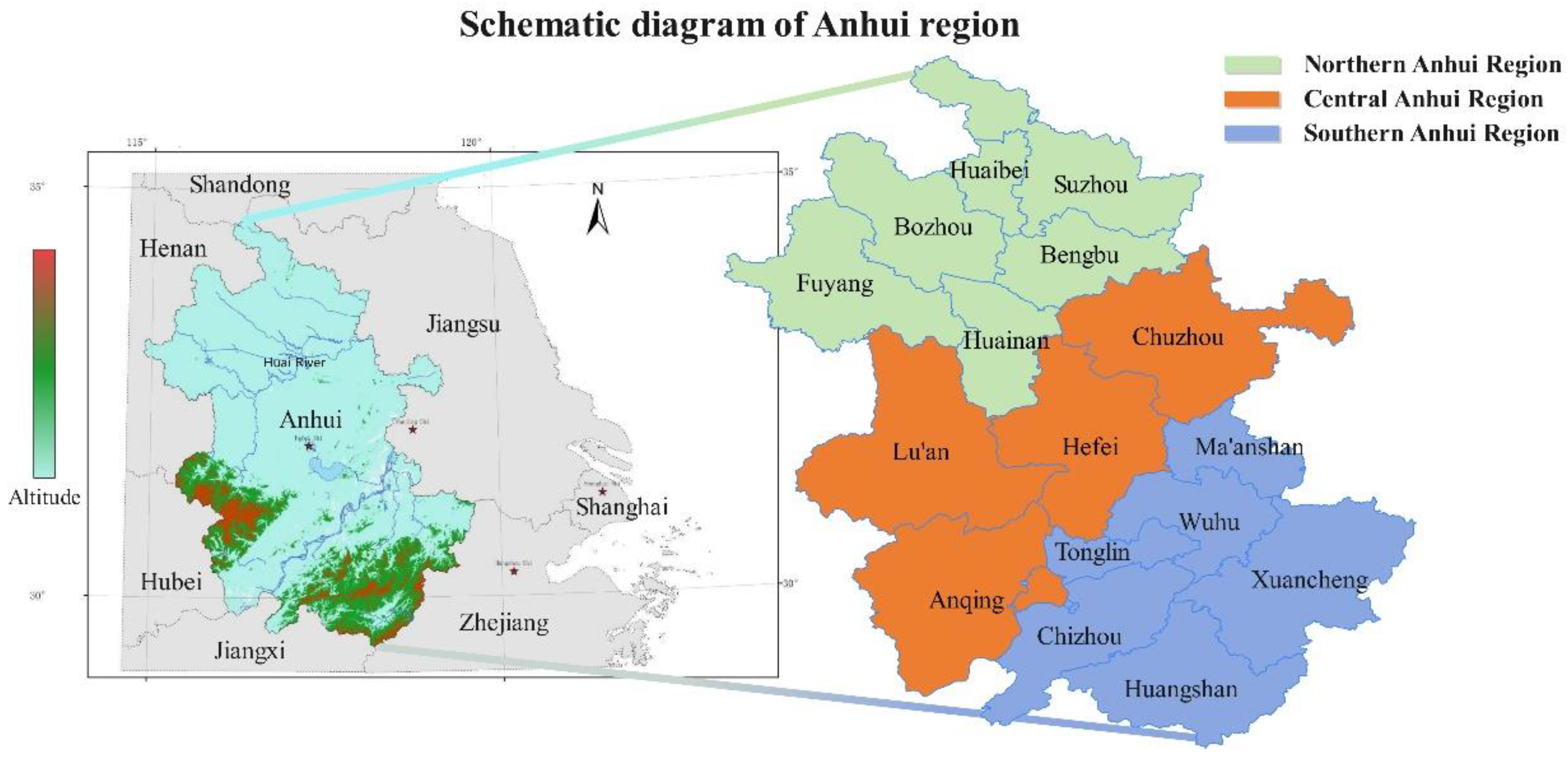
A comprehensive and accurate evaluation of regional AEE can be achieved by relying on the MinDS model and kernel density estimation, but the influencing factors of efficiency cannot be evaluated. To further explore the influencing factors of AEE and lay the foundation for proposing scientific optimization countermeasures, here a multiple regression model will be established, with the efficiency values measured by the MinDS model as the explanatory variables and the possible influencing factors as the explanatory variables. The efficiency values measured by the MinDS model considering undesired outputs take values in the range (0, 1), which are truncated data, when the parameter estimates would be biased and inconsistent if the model is regressed directly by ordinary least squares (OLS). To address the case of restricted values of the dependent variable, Tobin in 1958 proposed a regression model for estimating the restricted dependent variable by the maximum likelihood method, also known as the Tobit model [65], with the following expression:

$$Y_i={\alpha }_0+{\displaystyle \sum }_{i=1}^n{\alpha }_i{X}_i+{\epsilon }_i;i=1,2,3\cdots n$$

(4)

where $Y_i$ is the explained variables, i.e., the AEE value; $X_i$ is the explanatory variable; $a_i$ is the parameter to be estimated; ${\epsilon }_i$ is the random variable; and $n$ is the number of explanatory variables.

3.2. Research Case

In Section 3.1, the research constructs a data-driven AEE evaluation and optimization method. To further empirically demonstrate the effectiveness of this research process, this paper takes the Anhui Province in China as an example to show the implementation process of the above method. Anhui Province is a vitally important part of China’s agricultural production area and is of strategic importance to the country’s food security. Therefore, it was adopted as our empirical study area. Anhui Province is located in the east-central part of China and is the most dynamic component of the Yangtze River Delta. Anhui Province is about 570 km long from north to south and 450 km wide from east to west, with a total area of 140,100 km², accounting for approximately 1.45% of China’s land area. By the end of 2021, Anhui Province had a resident population of 61.13 million people. There are 16 cities in Anhui Province with a population greater than 1,300,000, namely, Hefei, Huabei, Bozhou, Suzhou, Bengbu, Fuyang, Huainan, Chuzhou, Lu’an, Ma’anshan, Wuhu, Xuancheng, Tongling, Chizhou, Anqing, and Huangshan. According to the surveying and mapping law of the People’s Republic of China, the 16 cities in Anhui Province can be spatially divided into northern, central, and southern Anhui [66]. Their districts are shown in Figure 1:

3.3. Variable Selection and Data

3.3.1. Variables for Measuring AEE

Based on the existing literature [12,31,32,38,39,40,41,42,43,44,45,46], we selected 11 indicators to construct the evaluation system of AEE, as shown in Table 1. The input variables mainly include two aspects of agricultural production, one is the production base, which includes arable land area, irrigated agricultural area, and agricultural employees; the other is the production process inputs including fertilizer, pesticide, agricultural plastic film, total agricultural machinery power, and agricultural diesel fuel. The desired output is composed of economic output and food output, which are represented by the disposable income of rural residents and gross agricultural output value, respectively. In the agricultural production process, the generation of desired output is usually accompanied by undesired output, and the undesired output in this study is the total amount of carbon emissions generated from engaging in the agricultural production process.

It has been well documented that both the agricultural production base and the agricultural production process contribute directly or indirectly to carbon emissions [67,68]. However, the main sources of carbon emissions considered by current scholars are tillage, agricultural machinery power, fertilizers, pesticides, agricultural films or mulches, and irrigation. To our knowledge, less literature considers carbon emissions from the use of diesel fuel. In this study, based on previous research [42,69,70,71], a more comprehensive table of carbon emission factors was constructed based the inclusion of diesel consumption (

Table 2. Carbon emission coefficients of the main carbon sources of AEE.

Carbon Source	Tillage	Irrigation	Diesel	Agricultural Machinery	Fertilizer	Pesticide	Agricultural Film
Coefficient	3.126 (kg/hm2)	25 (kg/hm2)	592.7 (kg/ton)	0.18 (kg/kw)	0.8956 (kg/kg)	4.9341 (kg/kg)	5.18 (kg/kg)

). The carbon emission calculation formula is given in Equation (5):

$$E={\displaystyle \sum }_{i=1}^{n}Ei={\displaystyle \sum }_{i=1}^{n}TiCi$$

(5)

E denotes total agricultural carbon emissions; Ei denotes carbon emissions from different agricultural inputs, Ti denotes various carbon sources, and Ci denotes the applicable carbon emission coefficient (Table 2).

3.3.2. Variables Affecting AEE

To provide the necessary scientific basis for the proposed optimal countermeasures, further scientific analysis of the influencing factors of AEE and their influencing mechanisms was needed. In this section, the AEE value measured by the MinDS model was taken as the dependent variable, and the possible influencing factors from economic, social, and demographic aspects, were selected as independent variables, and a Tobit regression analysis model was established to investigate the influence of each factor on AEE and its influencing mechanism. Through the study of the existing literature, six possible influencing factors were selected for this paper (

Table 3. Description of the variables characterizing the influencing factors.

Influencing Factors	Indicator Description	Abbreviation	Unit
Population Aggregation Level	Population density, total regional population/regional area	PAL	persons/km2
Education Level	Regional years of education per capita	EL	years
Urbanization Level	urban population/total population of the region	UL	%
Economic Development Level	Regional gross domestic product/total regional population	EDL	Yuan/person
Rural Water Supply Capacity	Regional rural piped water supply rate	RW	%
Village Management Level	Number of village committees established in region	VML	—

).

The proposed rationale for the six influencing factors and the possible influencing mechanisms are shown in Appendix A.

Combined with the existing studies, we believe that the above factors may have an impact on AEE. To eliminate the effect of heteroskedasticity, the natural logarithm of PAL, GPC, and VML was taken. The Tobit model to test the influence of the factors on AEE and their influence mechanism can be expressed as:

$$y_{it}={\beta }_0+{\beta }_{1}LnPA{L}_{it}+{\beta }_{2}E{L}_{it}+{\beta }_{3}U{L}_{it}+{\beta }_{4}LnGP{C}_{it}+{\beta }_5{\mathrm{RW}}_{it}+{\beta }_{6}Ln{\mathrm{VML}}_{it}+{\epsilon }_{it}$$

(6)

where i denotes the ith city of Anhui province, t presents the year between 2015 and 2020, $y_{it}$ stands for the Agricultural environmental efficiency, ${\beta }_i$ is the coefficient, and ${\epsilon }_i$ is the stochastic error.

3.3.3. Data Sources and Description

The data of input and output variables of AEE evaluation in Anhui Province and the data of influencing factors were obtained from Anhui Provincial Statistical Yearbook in 2015–2020. The descriptive statistics of these variables is presented in

Table 4. Descriptive statistics of all variables.

Variables	Minimum	Maximum	Mean	Standard Deviation
x1	94,380	1,255,265	557,991.146	341,274.8181
x2	10.4	227.7	82.421	52.264
x3	31,942	383,842	196,574.333	108,457.482
x4	1463	24,097	6061.333	4653.7418
x5	423	21,377	6222.635	5902.2107
x6	80.81	985.49	414.1158	254.85586
x7	6295	117,410	47,113.021	30,660.0038
x8	51.23	503.37	281.9784	151.88268
r1	9001	25,421	14,420.479	3743.3305
r2	323,100	3,386,281	1,508,622.396	864,611.3921
z1	22,273,108	379,431,334	155,396,589.2	99,067,364.67
PAL	135.7295809	828.1649033	488.9979248	210.8723087
EL	8.13	11.29	9.2058	0.67496
UL	0.37	0.82	0.5505	0.10221
EDL	16,121	115,623	49,754.156	23,098.9609
RW	0.5714	0.996	0.842711	0.1046328
VML	276	1764	908.625	418.1613

Data from the Anhui Provincial Statistical Yearbook in 2015–2020.

. The data of Anhui Provincial Statistical Yearbook is collected by the statistical bureaus of each city according to the uniform caliber and standard. The statistical data is to serve the decision-making of Chinese government and the research work of think tanks, the source of the data is credible and reliable.

4. Results

4.1. Evaluation Results of AEE

We entered all the inputs, expected outputs, and undesired outputs of DUM, into the MaxDEA 9 software. Then, we used the MinDS model and SBM model to calculate the AEE of 16 cities in the Anhui Province from 2015–2020. The calculation results are depicted in

Table 5. AEE evaluation results of 16 cities in Anhui Province based on MinDS model.

Region	2015	2016	2017	2018	2019	2020	Mean
Anqing	0.737176899	0.756793904	0.773761605	0.752062674	0.755928849	0.7248397	0.750093938
Bengbu	0.58986775	0.593182359	0.579884187	0.590245837	0.656443694	0.564447448	0.595678546
Bozhou	0.846036332	1	0.775948065	0.594890778	0.545084462	0.571754401	0.722285673
Chizhou	0.688164676	0.655149464	0.701873996	0.782966424	0.864379506	1	0.782089011
Chuzhou	0.629923299	0.654182841	0.671354327	0.690153186	0.747582172	0.792030206	0.697537672
Fuyang	0.717930352	0.748742202	0.624964986	0.830173182	0.901116847	1	0.803821262
Hefei	0.693375431	0.765890737	0.841765525	0.901299238	0.95909807	1	0.860238167
Huaibei	0.671202651	0.626439743	0.66893453	0.674083218	0.653283423	0.719512829	0.668909399
Huainan	0.444101309	0.470669371	0.484104041	0.476733982	0.567173138	0.609254471	0.508672719
Huangshan	0.590535175	0.752061508	0.829672831	0.869825605	0.910251368	1	0.825391081
Lu’an	0.711851545	0.75431589	0.766370726	0.755573149	0.857664478	1	0.807629298
Ma’anshan	0.802736687	0.821950202	0.833568245	0.854108458	0.903572054	1	0.869322608
Suzhou	0.494257839	0.531944112	0.566480534	0.585002382	0.599515188	0.62364269	0.566807124
Tongling	0.709830435	0.710674944	0.743167955	0.793129068	0.847332556	1	0.800689160
Wuhu	0.824960947	0.84841145	0.848106028	0.826709851	0.900563881	1	0.874792026
Xuancheng	0.74300186	0.750059964	0.808705234	0.799389514	0.879960012	1	0.830186097

Data from the MaxDEA 9 software analysis.

.

By comparing the data in Table 5 and

Table 6. AEE evaluation results of 16 cities in Anhui Province based on SBM model.

Region	2015	2016	2017	2018	2019	2020	Mean
Anqing	0.211286976	0.228906882	0.246741288	0.269749309	0.306464533	0.381906729	0.274175953
Bengbu	0.24141075	0.267606966	0.292685177	0.314075107	0.376805142	0.486095721	0.329779811
Bozhou	0.174289881	1	0.221132607	0.253237559	0.314271172	0.370807515	0.388956456
Chizhou	0.664045838	0.591390071	0.622010083	0.735978405	0.84437789	1	0.742967048
Chuzhou	0.220412641	0.236742452	0.256645139	0.283183645	0.30057585	0.380314396	0.279645687
Fuyang	0.22329406	0.251614849	0.317643687	0.291023199	0.417155269	1	0.416788511
Hefei	0.378154726	0.426298117	0.488221166	0.559882476	0.7532761	1	0.600972098
Huaibei	0.351321302	0.357507986	0.487988244	0.530750256	0.599130013	0.704770799	0.505244767
Huainan	0.200580882	0.214072279	0.233226199	0.265992322	0.27166645	0.3068305	0.248728105
Huangshan	0.579480169	0.61939152	0.662572986	0.748160209	0.858231922	1	0.744639468
Lu’an	0.190844672	0.214850769	0.252822181	0.28495916	0.351544883	1	0.382503611
Ma’anshan	0.476286079	0.497651996	0.522173559	0.531823329	0.605175699	1	0.605518444
Suzhou	0.121798837	0.127122077	0.141491842	0.153150436	0.170726826	0.189308285	0.150599717
Tongling	0.472400464	0.569645725	0.624418532	0.699598717	0.822706041	1	0.698128247
Wuhu	0.523089031	0.587778372	0.622996598	0.677975134	0.826518955	1	0.706393015
Xuancheng	0.434072908	0.529936554	0.613196241	0.658619428	0.797918298	1	0.672290571

Data from the MaxDEA 9 software analysis.

, it can be observed that the SBM model amplifies the improvement potential of the evaluated area, and the evaluated efficiency values are low compared to MinDS. It is also evident from Table 6 that there are some abnormal evaluation results in the SBM model, such as the large differences in Fuyang, Lu’an, and Ma’anshan in 2019–2020, with a sudden change to DEA effective with lower DEA efficiency values, while the data of Bozhou in 2016 are highly different from neighboring years, which are not in line with the normal development law. However, such anomalies do not appear in the evaluation results of MinDS. This comparison further corroborates the arguments presented in the previous section. The following analysis and discussion are based on the evaluation results of the MinDS model.

From the average value of AEE in Table 5, it can be observed that the 16 cities in Anhui Province are still some distance away from the effective AEE in 2015–2020. Wuhu city has the highest efficiency value, with an average value of 0.87, and three cities had an average AEE value less than 0.6, namely, Bengbu (0.59), Suzhou (0.56), and Huainan (0.50). The results of these calculations indicate that the AEE of some cities in Anhui Province is not high and there is still much space for improvement.

To better show the change trend of AEE in the three regions of the Anhui Province, this study divided it into northern, central, and southern Anhui, and plotted the change trend of AEE values from 2015–2020. There was an overall increasing trend of AEE in the three regions (Figure 2). Among them, the AEE of southern Anhui increased from 0.72 in 2015 to 1 in 2020, indicating that this region reached almost the best possible efficiency in 2020, compared to other regions. Moreover, the AEE of northern and central Anhui also improved to some extent. Comparing the three curves in Figure 2, we can clearly see that the AEE shows a clear geographical difference, with southern Anhui performing better than the other regions in terms of carbon emission reduction and sustainability of agricultural production. We can observe that the overall performance of AEE in Anhui Province is good and in a stable growth trend, and that the growth rate gradually increased from 2017–2020 (Figure 2).

4.2. Distribution Characteristics and Dynamic Evolution of AEE

To further reveal the spatial distribution and evolutionary trends of AEE in Anhui Province, the non-parametric kernel density estimation of Gaussian normal distribution was calculated using the Stata 16.0 statistical software for 2015, 2017, 2019, and 2020 (Figure 3). The overall position of the nuclear density curve shows a trend of shifting to the right from 2015–2020, indicating that the AEE in Anhui Province has generally been increasing during the examined period (Figure 3), which is consistent with the results of the previously described analysis.

4.3. Influencing Factors of AEE

Using the Stata 16.0 software, the Tobit regression method was applied to test the influence mechanism of the influencing factors hypothesized in Section 3.3.2. The results of the regression analysis are shown in

Table 7. Results of Tobit regression. See Table 3 for factor abbreviations.

Independent Variable	Coefficient	Standard Error	T-Value	p-Value
PAL	−0.0293694	0.0263043	−1.12	0.267
EL	−0.089639	0.0394649	−2.27	0.026
UL	0.0043063	0.0028985	1.49	0.141
EDL	0.1790713	0.0622738	2.88	0.005
RW	0.4611818	0.1460967	3.16	0.002
VML	0.0930493	0.0308424	3.02	0.003

. All explanatory variables except PAL and UL were significant at the 1% and 5% levels, which indicates that EL, EDL, RW, and VML, have strong explanatory power for the disparity in AEE. Among them, EDL, RW, and VML, had a significant positive effect and EL a significant negative effect (Table 7).

5. Discussion

This study constructed a data-driven AEE evaluation and optimization process, and empirically demonstrated the influencing factors of AEE using scientific quantitative analysis, which lays the foundation for more accurate policy recommendations. The evaluation results and influencing factors are further analyzed and discussed below.

5.1. Discussion on AEE Evaluation Results

In order to look at each city, Wuhu, Tongling, Ma’anshan, Hefei, Xuancheng, Huangshan, Lu’an, and Fuyang, performed better overall, with an average AEE value reaching 0.8 or more during the study period. Wuhu had the highest average AEE (0.87), which indicates that it has a high efficiency and a reasonable allocation of resources in the process of agricultural production, while also paying attention to controlling carbon emissions. Moreover, there were nine cities with an efficiency score of 1.0 in 2020, namely Wuhu, Ma’anshan, Hefei, Huangshan, Lu’an, Xuancheng, Tongling, Chizhou, and Fuyang. This indicates that these cities achieved effective AEE in 2020, including the best relative resource efficiency, agricultural production efficiency, and reasonable carbon emissions. With the exception of Anqing, Bozhou, and Bengbu, most of the cities improved their AEE to different degrees during the study period, which indicates that the utilization of agricultural resources and production technology are improving, that people’s awareness of environmental protection is gradually strengthening, and that the capacity for sustainable development is improving. Huangshan showed the largest improvement, with an AEE increase of 0.40 during the study period, while Chizhou, Lu’an, Fuyang, and Hefei, also gained significant improvements, with increases >0.25.

From the three regions of Anhui Province, the average efficiency of northern, central and southern Anhui was 0.64, 0.78, and 0.83, respectively. During the examination period, all regions showed an increasing trend in AEE values, with northern, central, and southern Anhui increasing by 8.64%, 26.86% and 37.6%, respectively. This means that the southern part of Anhui was better than the other regions in implementing measures to reduce carbon emissions and promote sustainable agricultural development, while the northern part of Anhui Province has more space for improvement.

Overall, AEE in Anhui Province showed an increasing trend, from 0.68 in 2015 to 0.85 in 2020, with a growth rate of about 24.87% (Figure 2). The growth rate of AEE in Anhui increased gradually from 0.005 in 2016–2017 to 0.066 in 2019–2020. Firstly, this could be attributed to the rapid development of the economic level in the province, in which the average annual GDP growth reached 8.2% from 2015–2020 [72]. Secondly, it could be due to the improvement in agricultural technology, which promotes the full utilization of production factors in the production process and reduces their redundancy rate, resulting in significantly increases in the desired output and reduction of undesired outputs [73]. Lastly, the implementation of carbon emission verification and related monitoring work in Anhui Province from 2016–2020 [73,74] would have strengthened environmental awareness and effectively curbed the carbon emissions in the agricultural production process.

5.2. Discussion of the Spatial Distribution and Dynamic Evolution of AEE

Kernel density estimation was carried out to further reveal the spatial distribution characteristics and dynamic evolution of AEE in Anhui Province. The center of the density curve of AEE shifted to the right from 2015–2020 (Figure 3), and the AEE in Anhui Province increased during the examination period, which is consistent with the above findings. Compared with 2015, the width and height of the AEE density curve in 2020 continued to decrease, indicating that the variation of AEE in Anhui Province decreased during the examination period. The number of peaks gradually changed from one to two. The density curves in 2019–2020 show a pattern of coexistence of main peaks and secondary peaks, which correspond to cities with higher and lower AEE, respectively. Furthermore, the density value of the main peak is significantly higher than that of the secondary peak. These phenomena suggest that the AEE of the Anhui Province is gradually splitting into two poles. This may be due to the low AEE in the economically less-progressive regions, where less attention has been paid to environmental protection and agricultural production efficiency [75]. In the more economically developed regions, the AEE is higher due to reasonable agricultural production methods and appropriate agricultural inputs. Anhui Province shows a clear situation of relative poverty in the north and relative affluence in the south, as reflected in GDP values, which will inevitably lead to a polarization of AEE.

5.3. Discussion of the Influencing Factors of AEE

To explore the influencing factors that cause the differences in AEE between cities, and to lay the foundation for the proposed optimization measures, it is necessary to further discuss and analyze the regression results of the influencing factors.

The population aggregation levels (PAL) showed a negative but insignificant correlation in the coefficients, and therefore did not have a significant impact on the differences in AEE during the examined period. This is different from some previous research [76,77], but is similar to the findings of Zhang’s study [53].

It is worth noting that the educational level (EL) of the regional population shows a significant negative correlation with AEE. This indicates that as the education level of the regional population increases, the AEE decreases, which is opposite to previous findings [78,79,80,81]. This result is worthy of attention and can be further explored. In many countries worldwide, including China, there is often a large developmental gap between rural and urban areas, and rural areas are relatively poor [82,83,84]. Rural residents who have received more education, especially more knowledgeable young people, often choose to go to cities in search of better opportunities, which leads to a loss of agricultural talent [85,86]. The higher the level of education, the more serious the problem of rural population depletion, which ultimately results in a high proportion of elderly persons and children in the population structure of many villages [87]. This situation will be detrimental to agricultural production activities, and to the attention given to environmental protection and reduction of carbon emissions in agricultural production processes.

The effect of urbanization level (UL) on AEE is positive, and may increase regional AEE. However, due to the high complexity and multidimensionality of Chinese society, including the Anhui Province [88], this effect is insignificant from the regression results, which differs from the outcomes of some previous studies [41,89].

The economic development level (EDL) of the region shows a significant positive correlation with the AEE of the region, which supports the findings of some previous scholars [41,90,91,92]. Based on previous research, it is known that regions with higher levels of economic development have great advantages in terms of production factors such as input capital, agricultural science and technology, and agricultural management policies, and thus can better achieve improved agricultural production conditions and profitability [92]. Moreover, economic growth can lead to a significant increase in urban construction land and a sharp decrease in the extent of agricultural land [89], which to some degree promotes the transformation of agricultural intensification and improves agricultural production efficiency.

Rural water (RW) supply capacity showed a significant positive correlation with AEE, which is consistent with previous findings [79,93,94]. This suggests that the regional AEE can be improved by increasing the rate of piped water supply in rural areas, and the effect of this improvement is significant. Popova pointed out that the provision of convenient and uninterrupted water supply to agricultural areas is one of the factors that ensure food security [95]. Considering the limited availability of water resources, the government should investigate and forecast the demand for water resources in agricultural production for each region, and then develop management plans to further improve the efficiency of water use and promote the rational use of water resources [96,97].

As presented in Table 7, the level of village management (VML) showed a significant positive correlation with regional AEE. This indicates that village committees contribute significantly to the promotion of regional agricultural production and environmental sustainability, which supports previous findings [76,98]. According to Chinese government policy, village committees are required to manage the land and other property belonging to the village farmers’ collective, educate villagers to use natural resources wisely, and protect and improve the ecological environment. Based on the results of the analysis, it is shown that currently, village committees effectively implement these responsibilities.

5.4. Innovation and Advantages

Sustainable development of agriculture is an important part of sustainable development worldwide. To fill the existing knowledge gap, better evaluate and optimize AEE, and promote the sustainable development of agriculture, this study aimed to construct a data-driven method for evaluating and optimizing AEE under carbon emission constraints. This study accomplishes this research objective and, at the same time, proposes the following three innovations and advantages over the previous literature.

First, considering the obvious disadvantages and unreasonable aspects of the DEA model commonly used in the previous literature [31,32,33,36,41,53,54,99,100], this study constructs a more accurate and precise MinDS evaluation model, which improves the accuracy and scientific basis of the evaluation results. This research incorporates the kernel density estimation analysis method in the evaluation of AEE, which can present the dynamic evolution trend and distribution characteristics of AEE more intuitively. Thus, a more accurate and comprehensive AEE evaluation is achieved compared with previous literature.

Second, regarding the design of evaluation indicators, compared with previous literature [12,31,32,38,39,40,41,42,43,44,45,46], this study constructs a more comprehensive AEE evaluation index system, which incorporates both basic agricultural production inputs and production process inputs in the input indicators. To better reflect the agricultural sustainability attributes of AEE, the total agricultural output value and per capita income of farmers were taken as the desired output indicators, and the total carbon emissions in agricultural production were taken as the undesired output, to fully consider the carbon emissions in the agricultural production process. At the same time, this study makes up for the neglect of carbon emissions from diesel consumption in the carbon emission calculation, to lay a foundation for more accurate AEE calculations.

Finally, AEE evaluation was conducted to optimize AEE more accurately. Compared with previous research [33,46,47,48,49,51,52], this study constructed a more scientific data-driven AEE optimization process. Based on the results of AEE evaluation and analysis, a scientific mathematical method is used to empirically demonstrate the influencing factors of AEE and their influence mechanisms, which provides a more scientific and accurate theoretical basis for optimization strategy proposals.

5.5. Research Contribution

Currently, the world is facing severe challenges in agricultural production and dealing with the climate crisis [18,19,20,21,22,23,24,25,26,27,28]. Studying AEE from a low-carbon perspective is important for addressing these challenges and promoting global sustainable development. Specifically, this study makes the following three contributions. First, it expands the research methodology of AEE evaluation, and constructs a combined dynamic and static evaluation and analysis method. This not only improves the accuracy and comprehensiveness of the evaluation results, but also enriches the theoretical basis of the field and provide insights for better evaluation of AEE under environmental constraints. Secondly, the study constructs a comprehensive AEE input-output evaluation index system under carbon emission constraints, and the evaluation results can fully reflect the carbon emission constraints. The evaluation results can provide the necessary scientific basis for improving agricultural production efficiency and limiting carbon emissions. Simultaneously, the study introduces a detailed method of measuring carbon emissions in agricultural production, which can be used as a reference for other scholars. Finally, this study constructs a data-driven AEE evaluation and optimization process. Several influencing factors of AEE are empirically analyzed from social, economic, and demographic perspectives, and action strategies for optimizing AEE are proposed based on these key factors. This contributes to improving agricultural production efficiency, reducing environmental pollution, controlling carbon emissions, and promoting the sustainable development of agriculture.

6. Summary and Policy Suggestions

Currently, agricultural production is facing serious challenges due to the increasing global population, water shortages, and shrinking arable land. Simultaneously, global sustainable development is affected by environmental pollution and severe carbon emissions in agricultural production. Therefore, we propose the research objective of constructing a data-driven approach to evaluate and optimize AEE under carbon emission constraints. We accomplished this research task, specifically, as follows. Firstly, we constructed a more comprehensive input-output evaluation index system, including carbon emissions as undesired outputs, and more accurately measure the total carbon emissions of regional agriculture. Secondly, we applied the MinDS model to evaluate the AEE more accurately, and analyzed the regional distribution characteristics and evolution of AEE by using the kernel density estimation method. Finally, we constructed a data-driven process, validated the hypothesized six AEE influencing factors and analyzed their influence mechanisms. The validation results showed that PAL and UL were inconsistent with the hypothesis, and EL, EDL, RW, and VML, were consistent with the hypothesis, and had strong explanatory power for the disparity in AEE. Based on the influencing factors and influence mechanisms, we proposed countermeasures to optimize AEE.

6.1. Policy Suggestions

To further optimize the AEE, the following five countermeasures are proposed based on the efficiency evaluation results and the study of influencing factors: (1) for areas where the AEE is not effective, there is a general problem of too much input and too much undesired output. It is necessary to further increase the investment in agricultural research, research and development of low-energy, and high-efficiency machinery and equipment, improve resource utilization, and reduce undesired output emissions; (2) the evaluation results of AEE show obvious regional differences. This is influenced by the level of regional economic development. AEE can be improved by strengthening inter-regional cooperation and exchange, by actively introducing advanced low-carbon agricultural technologies, and by learning and implementing ecological agricultural experience from developed regions; (3) actively increase collective economic income, raise the income level of rural residents, and reduce the loss of young talents. Implement a flexible and effective talent policy to fully attract young talents, entrepreneurs, and technicians, who have already left the country to return to rural areas, and encourage them to contribute to agricultural production. In addition to encouragement, young people also want to feel financially incentivized. This can be done by offering scholarship programs to students who study agriculture and environmental professions and return to their home regions to participate in agricultural development. This could be very rewarding; (4) strengthen the construction of agricultural infrastructure conditions and networks, with special attention to improving rural water supply capacity and the practicality of water use in the agricultural production process. In addition, considering the possibility of future climate extremes, it is necessary to construct dynamic forecasting approaches and to take some necessary government interventions when facing years of extreme high or low rainfall; and (5) to give full recognition to the crucial role of village committees in the development of agro-ecology. We should actively guide farmers to fully understand the advantages of ecological agriculture and change their traditional farming approaches. Establishing appropriate incentives and compensation mechanisms to motivate farmers to develop green agriculture and gradually develop a low-carbon lifestyle will benefit multiple role-players.

6.2. Research Limitations

There are three limitations in this study: (1) the results of AEE evaluation may vary considerably between different crops in agricultural production, and the study did not take this into account; (2) the spatial interactions of AEE were not analyzed; and (3) many other factors may also affect AEE, and although this study verified different influencing factors, from social, economic, and population perspectives, other factors can still be further considered to improve future models for evaluating AEE.

6.3. Research Outlook

First, the study can be further refined to analyze the AEE of different crops and their proportional representation regionally, which can contribute to the improvement of production efficiency and reduction of carbon emissions for different crops. Secondly, the spatial correlation of AEE and its drivers can be further explored by combining spatial autocorrelation models and geographic detectors. Finally, more diverse influencing factors can be verified in the context of regional or national agricultural development to lay the theoretical foundation for optimizing AEE and proposing sustainable development policies.

References

1. Marchand, S.; GUO, H. The environmental efficiency of non-certified organic farming in China: A case study of paddy rice production. China Econ. Rev. 2014, 31, 201–216. [Google Scholar] [CrossRef]
2. Tyteca, D. On the Measurement of the Environmental Performance of Firms—A Literature Review and a Productive Efficiency Perspective. J. Environ. Manag. 1996, 46, 281–308. [Google Scholar] [CrossRef]
3. Sinkin, C.; Wright, C.J.; Burnett, R.D. Eco-efficiency and firm value. J. Account. Public Pol. 2008, 27, 167–176. [Google Scholar] [CrossRef]
4. Burnett, R.D.; Hansen, D.R. Ecoefficiency: Defining a role for environmental cost management. Account. Organ. Soc. 2008, 33, 551–581. [Google Scholar] [CrossRef]
5. Li, X.H.; Zhu, X.G.; Li, J.S.; Gu, C. Influence of Different Industrial Agglomeration Modes on Eco-Efficiency in China. Int. J. Environ. Res. Public Health 2021, 18, 13139. [Google Scholar] [CrossRef]
6. Zhou, Y.; Liu, Z.; Liu, S.; Chen, M.; Zhang, X.; Wang, Y. Analysis of industrial eco-efficiency and its influencing factors in China. Clean Technol. Environ. 2020, 22, 2023–2038. [Google Scholar] [CrossRef]
7. Soliman, T.; Djanibekov, U. Assessing dairy farming eco-efficiency in New Zealand: A two-stage data envelopment analysis. N. Z. J. Agr. Res. 2021, 64, 411–428. [Google Scholar] [CrossRef]
8. Tang, M.G.; Li, Z.; Hu, F.X.; Wu, B.J. How does land urbanization promote urban eco-efficiency? The mediating effect of industrial structure advancement. J. Clean. Prod. 2020, 272, 122798. [Google Scholar] [CrossRef]
9. Liu, Q.F.; Song, J.P.; Dai, T.Q.; Xu, J.H.; Li, J.M.; Wang, E.R. Spatial Network Structure of China’s Provincial-Scale Tourism Eco-Efficiency: A Social Network Analysis. Energies 2022, 15, 1324. [Google Scholar] [CrossRef]
10. Li, Y.L.; Zuo, Z.L.; Xu, D.Y.; Wei, Y. Mining Eco-Efficiency Measurement and Driving Factors Identification Based on Meta-US-SBM in Guangxi Province, China. Int. J. Environ. Res. Public Health 2021, 18, 5397. [Google Scholar] [CrossRef]
11. Cui, S.N.; Wang, Y.Q.; Zhu, Z.W.; Zhu, Z.H.; Yu, C.Y. The impact of heterogeneous environmental regulation on the energy eco-efficiency of China’s energy-mineral cities. J. Clean Prod. 2022, 350, 131553. [Google Scholar] [CrossRef]
12. Luo, M.C.; Liu, F.; Chen, J.Q. Data-Driven Evaluation and Optimization of Agricultural Sustainable Development Capability: A Case Study of Northern Anhui. Processes 2021, 9, 2036. [Google Scholar] [CrossRef]
13. Wrzaszcz, W.; Zielinski, M. Sustainable Development of Agriculture in Poland—Towards Organization and Biodiversity Improvement? Eur. J. Sustain. Dev. 2022, 11, 87–100. [Google Scholar] [CrossRef]
14. Abdar, Z.K.; Amirtaimoori, S.; Mehrjerdi, M.; Boshrabadi, H.M. A composite index for assessment of agricultural sustainability: The case of Iran. Environ. Sci. Pollut. R 2022, 29, 47337–47349. [Google Scholar] [CrossRef]
15. Hamid, S.; Wang, K. Environmental total factor productivity of agriculture in South Asia: A generalized decomposition of Luenberger-Hicks-Moorsteen productivity indicator. J. Clean Prod. 2022, 351, 131483. [Google Scholar] [CrossRef]
16. Xu, P.; Jin, Z.H.; Ye, X.X.; Wang, C. Efficiency Measurement and Spatial Spillover Effect of Green Agricultural Development in China. Front. Environ. Sci. 2022, 10, 909321. [Google Scholar] [CrossRef]
17. Rosano-Pena, C.; Teixeira, J.R.; Kimura, H. Eco-efficiency in Brazilian Amazonian agriculture: Opportunity costs of degradation and protection of the environment. Environ. Sci. Pollut. R 2021, 28, 62378–62389. [Google Scholar] [CrossRef]
18. Natesan, V.T.; Mani, P.; Prasad, T.; Krishna, J.M.; Sekar, S. Applications of Thin Layer Modelling Techniques and Advances in Drying of Agricultural Products. AIP Conf. Proc. 2020, 2311, 090025. [Google Scholar] [CrossRef]
19. Gong, X.H.; Zhang, H.B.; Ren, C.F.; Sun, D.Y.; Yang, J.T. Optimization allocation of irrigation water Resources based on crop water requirement under considering effective precipitation and uncertainty. Agr. Water Manag. 2020, 239, 106264. [Google Scholar] [CrossRef]
20. Imoro, Z.A.; Imoro, A.Z.; Duwiejuah, A.B.; Abukari, A. Harnessing Indigenous Technologies for Sustainable Management of Land, Water, and Food Res.ources Amidst Climate Change. Front. Sustain. Food Syst. 2021, 5, 691603. [Google Scholar] [CrossRef]
21. Yang, B.; Wang, Z.Q.; Zou, L.; Zou, L.L.; Zhang, H.W. Exploring the eco-efficiency of cultivated land utilization and its influencing factors in China’s Yangtze River Economic Belt, 2001-2018. J. Environ. Manag. 2021, 294, 112939. [Google Scholar] [CrossRef] [PubMed]
22. Miceikiene, A.; Krikstolaitis, R.; Nausediene, A. An assessment of the factors affecting environmental pollution in agriculture in selected countries of Europe. Transform. Bus Econ. 2021, 20, 93–110. [Google Scholar]
23. Wyckhuys, K.; Zou, Y.; Wanger, T.C.; Zhou, W.W.; Gc, Y.D.; Lu, Y.H. Agro-ecology science relates to economic development but not global pesticide pollution. J. Environ. Manag. 2022, 307, 114529. [Google Scholar] [CrossRef] [PubMed]
24. Ali, R.; Ishaq, R.; Bakhsh, K.; Yasin, M.A. Do Agriculture Technologies Influence Carbon Emissions in Pakistan? Evidence based on ARDL technique. Environ. Sci. Pollut. R 2022, 29, 43361–43370. [Google Scholar] [CrossRef] [PubMed]
25. Li, M.; Liu, S.; Sun, Y.; Liu, Y. Agriculture and animal husbandry increased carbon footprInt. on the Qinghai-Tibet Plateau during past three decades. J. Clean Prod. 2021, 278, 123963. [Google Scholar] [CrossRef]
26. IPCC. Climate Change and Land. Available online: https://www.ipcc.ch/srccl/chapter/chapter-2/ (accessed on 1 August 2022).
27. Guo, L.L.; Guo, S.H.; Tang, M.Q.; Su, M.Y.; Li, H.J. Financial Support for Agriculture, Chemical Fertilizer Use, and Carbon Emissions from Agricultural Production in China. Int. J. Environ. Res. Public Health 2022, 19, 7155. [Google Scholar] [CrossRef]
28. Yasmeen, R.; Tao, R.; Shah, W.U.H.; Padda, I.U.H.; Tang, C. The nexuses between carbon emissions, agriculture production efficiency, research and development, and government effectiveness: Evidence from major agriculture-producing countries. Environ. Sci. Pollut. R 2022, 29, 52133–52146. [Google Scholar] [CrossRef]
29. Banker, R.D.; Charnes, A.; Cooper, W.W. Some Models for Estimating Technical and Scale Inefficiencies in Data Envelopment Analysis. Manag. Sci. 1984, 30, 1078–1092. [Google Scholar] [CrossRef]
30. Charnes, A.; Cooper, W.W.; Rhodes, E. Measuring the efficiency of decision making units. Eur. J. Oper. Res. 1978, 2, 429–444. [Google Scholar] [CrossRef]
31. YougbarÃ, J.W. Analysis of Agricultural Performance in Burkina Faso Using Data Envelopment Analysis. Eur. J. Pure Appl. Math. 2021, 14, 366–379. [Google Scholar] [CrossRef]
32. Flegl, M.; Jiménez-Bandala, C.A.; Sánchez-Juárez, I.; Matus, E. Analysis of production and investment efficiency in the Mexican food industry: Application of two-stage DEA. Czech J. Food Sci. 2022, 40, 109–117. [Google Scholar] [CrossRef]
33. Singh, G.; Singh, P.; Sodhi, G.P.S.; Tiwari, D. Energy auditing and data envelopment analysis (DEA) based optimization for increased energy use efficiency in wheat cultivation (Triticum aestium L.) in north-western India. Sustain. Energy Technol. Assess. 2021, 47, 101453. [Google Scholar] [CrossRef]
34. Li, G.Z.; Tang, D.C.; Boamah, V.; Pan, Z.W. Evaluation and Influencing Factors of Agricultural Green Efficiency in Jianghuai Ecological Economic Zone. Sustainability 2022, 14, 30. [Google Scholar] [CrossRef]
35. Li, Q.; Wu, X.; Zhang, Y.; Wang, Y. The Effect of Agricultural Environmental Total Factor Productivity on Urban-Rural Income Gap: Integrated View from China. Sustainability 2020, 12, 3327. [Google Scholar] [CrossRef]
36. Pan, W.T.; Zhuang, M.E.; Zhou, Y.Y.; Yang, J.J. Research on sustainable development and efficiency of China’s E-Agriculture based on a data envelopment analysis-Malmquist model. Technol. Forecast. Soc. 2021, 162, 120298. [Google Scholar] [CrossRef]
37. Xie, H.L.; Zhang, Y.W.; Choi, Y. Measuring the Cultivated Land Use Efficiency of the Main Grain-Producing Areas in China under the Constraints of Carbon Emissions and Agricultural Nonpoint. Source Pollution. Sustainability 2018, 10, 1932. [Google Scholar] [CrossRef]
38. Gu, H.; Hu, Q.; Wang, T. Payment for Rice Growers to Reduce Using N Fertilizer in the GHG Mitigation Program Driven by the Government: Evidence from Shanghai. Sustainability 2019, 11, 1927. [Google Scholar] [CrossRef]
39. Long, X.; Luo, Y.; Sun, H.; Tian, G. Fertilizer using Intensity and environmental efficiency for China’s agriculture sector from 1997 to 2014. Nat. Hazards 2018, 92, 1573–1591. [Google Scholar] [CrossRef]
40. Skevas, T.; Serra, T. Derivation of netput shadow prices under different levels of pest pressure. J. Prod. Anal. 2017, 48, 25–34. [Google Scholar] [CrossRef]
41. Guo, Y.; Tong, L.; Mei, L. Spatiotemporal characteristics and influencing factors of agricultural eco-efficiency in Jilin agricultural production zone from a low carbon perspective. Environ. Sci. Pollut. R 2022, 29, 29854–29869. [Google Scholar] [CrossRef]
42. Kuang, B.; Lu, X.; Zhou, M.; Chen, D. Provincial cultivated land use efficiency in China: Empirical analysis based on the SBM-DEA model with carbon emissions considered. Technol. Forecast. Soc. 2020, 151, 119874. [Google Scholar] [CrossRef]
43. Faere, R.; Grosskopf, S.; Lovell, C.A.K.; Pasurka, C. Multilateral Productivity Comparisons When Some Outputs are Undesirable: A Nonparametric Approach. Rev. Econ. Stat. 1989, 71, 90. [Google Scholar] [CrossRef]
44. Knox Lovell, C.A.; Pastor, J.T.; Turner, J.A. Measuring macroeconomic performance in the OECD: A comparison of European and non-European countries. Eur. J. Oper Res. 1995, 87, 507–518. [Google Scholar] [CrossRef]
45. Tang, X.; Lu, C.; Meng, P.; Cheng, W. Spatiotemporal Evolution of the Environmental Adaptability Efficiency of the Agricultural System in China. Sustainability 2022, 14, 3685. [Google Scholar] [CrossRef]
46. Dong, G.; Wang, Z.; Mao, X. Production efficiency and GHG emissions reduction potential evaluation in the crop production system based on emergy synthesis and nonseparable undesirable output DEA: A case study in Zhejiang Province, China. PLoS ONE 2018, 13, e206680. [Google Scholar] [CrossRef]
47. Bibi, Z.; Khan, D.; Haq, I.U. Technical and environmental efficiency of agriculture sector in South Asia: A stochastic frontier analysis approach. Environ. Dev. Sustain. 2021, 23, 9260–9279. [Google Scholar] [CrossRef]
48. Gai, Z.; Sun, P.; Zhang, J. Cultivated Land Utilization Efficiency and Its Difference with Consideration of Environmental ConstraInt.s in Major Grain Producing Area. Econ. Geogr. 2017, 37, 163–171. [Google Scholar] [CrossRef]
49. Qiu, L.; Zhu, J.; Pan, Y.; Wu, S.; Dang, Y.; Xu, B.; Yang, H. The positive impacts of landscape fragmentation on the diversification of agricultural production in Zhejiang Province, China. J. Clean Prod. 2020, 251, 119722. [Google Scholar] [CrossRef]
50. Rodríguez, C.; Wiegand, K. Evaluating the trade-off between machinery efficiency and loss of biodiversity-friendly habitats in arable landscapes: The role of field size. Agric. Ecosyst. Environ. 2009, 129, 361–366. [Google Scholar] [CrossRef]
51. Kaiwei, Z.; Zhen, L.; Xunmin, O.; Liangping, H.; Jinchai, L. Evaluation of energy-oriented utilization potential of main Chinese crop Res.idues based on soil protection functions. Chin. J. Ecol. Agric. 2017, 25, 276–286. [Google Scholar] [CrossRef]
52. Ginni, G.; Kavitha, S.; Kannah, Y.; Bhatia, S.K.; Kumar, A.; Rajkumar, M.; Kumar, G.; Pugazhendhi, A.; Chi, N.T.L. Valorization of agricultural Res.idues: Different biorefinery routes. J. Environ. Chem. Eng. 2021, 9, 105435. [Google Scholar] [CrossRef]
53. Zhang, X.; Zheng, X. Analyzing agricultural ecological efficiency in Weihai City based on the SBM, STIRPAT and SLM models. J. Physics. Conf. Ser. 2021, 1941, 12030. [Google Scholar] [CrossRef]
54. Wen, L.; Li, H. Estimation of agricultural energy efficiency in five provinces: Based on data envelopment analysis and Malmquist index model. Energy Sources Part A Recovery Util. Environ. Eff. 2019, 44, 2900–2913. [Google Scholar] [CrossRef]
55. Tone, K. Variations on the theme of slacks-based measure of efficiency in DEA. Eur. J. Oper. Res. 2010, 200, 901–907. [Google Scholar] [CrossRef]
56. Tone, K. A slacks-based measure of efficiency in data envelopment analysis. Eur. J. Oper. Res. 2001, 130, 498–509. [Google Scholar] [CrossRef]
57. Aparicio, J.; Ruiz, J.L.; Sirvent, I. Closest targets and minimum distance to the Pareto-efficient frontier in DEA. J. Prod. Anal. 2007, 28, 209–218. [Google Scholar] [CrossRef]
58. Smith, P.; Martino, D.; Cai, Z.; Gwary, D.; Janzen, H.; Kumar, P.; McCarl, B.; Ogle, S.; O’Mara, F.; Rice, C.; et al. Greenhouse gas mitigation in agriculture. Philos. Trans. R. Soc. B Biol. Sci. 2008, 363, 789–813. [Google Scholar] [CrossRef]
59. Power, A.G. Ecosystem services and agriculture: Tradeoffs and synergies. Philos. Trans. R. Soc. B Biol. Sci. 2010, 365, 2959–2971. [Google Scholar] [CrossRef]
60. Gao, P.; Yue, S.; Chen, H. Carbon emission efficiency of China’s industry sectors: From the perspective of embodied carbon emissions. J. Clean Prod. 2021, 283, 124655. [Google Scholar] [CrossRef]
61. Wang, X.; Zhu, Y.; Sun, H.; Jia, F. Production decisions of new and remanufactured products: Implications for low carbon emission economy. J. Clean Prod. 2018, 171, 1225–1243. [Google Scholar] [CrossRef]
62. Xue, S.; Yang, T.; Zhang, K.; Feng, J. Spatial effect and influencing factors of agricultural water environmental efficiency in china. Appl. Ecol. Env. Res. 2018, 16, 4491–4504. [Google Scholar] [CrossRef]
63. Keivani, E.; Abbaspour, M.; Abedi, Z.; Ahmadian, M. Promotion of Low-Carbon Economy through Efficiency Analysis: A Case Study of a Petrochemical Plant. Int. J. Environ. Res. 2021, 15, 45–55. [Google Scholar] [CrossRef]
64. Martinho, V.J.P.D. Efficiency, total factor productivity and returns to scale in a sustainable perspective: An analysis in the European Union at farm and regional level. Land Use Policy 2017, 68, 232–245. [Google Scholar] [CrossRef]
65. Tobin, J. Estimation of Relationships for Limited Dependent Variables. Econometrica 1958, 26, 24–36. [Google Scholar] [CrossRef]
66. The National People’s Congress of the People’s Republic of China. Survey and Mapping Law of the People’s Republic of China. Available online: http://www.npc.gov.cn/zgrdw/npc/xinwen/2017-04/27/content_2020927.htm (accessed on 25 July 2022).
67. Schlesinger, W.H. Biogeochemical constraInt.s on climate change mitigation through regenerative farming. Biogeochemistry 2022. [Google Scholar] [CrossRef]
68. Tiefenbacher, A.; Sandén, T.; Haslmayr, H.; Miloczki, J.; Wenzel, W.; Spiegel, H. Optimizing Carbon Sequestration in Croplands: A Synthesis. Agronomy 2021, 11, 882. [Google Scholar] [CrossRef]
69. West, T.O.; Marland, G.; ORNL, O.R.N.L. A synthesis of carbon sequestration, carbon emissions, and net carbon flux in agriculture: Comparing tillage practices in the United States. Agric. Ecosyst. Environ. 2002, 91, 217–232. [Google Scholar] [CrossRef]
70. Dubey, A.; Lal, R. Carbon FootprInt. and Sustainability of Agricultural Production Systems in Punjab, India, and Ohio, USA. J. Crop Improv. 2009, 23, 332–350. [Google Scholar] [CrossRef]
71. National Center for Climate Change Strategy and International Cooperation (NCSC). Guidelines for the Preparation of Provincial Greenhouse Gas Inventories. Available online: http://www.ncsc.org.cn/SY/tjkhybg/202003/t20200319_769763.shtml (accessed on 13 July 2022).
72. Anhui Net. The Average Annual Growth Rate of Anhui’s GDP in the 13th Five-Year Plan Period Is 8.2%. Available online: http://www.ahwang.cn/anhui/20201226/2176599.html (accessed on 29 July 2022).
73. Anhui Province Government. General Office of Anhui Provincial People’s Government on the Issuance of Anhui Provincial Agricultural Modernization Promotion Plan (2016–2020). Available online: https://www.ah.gov.cn/public/1681/7966841.html (accessed on 29 July 2022).
74. Anhui Province Government. General Office of Anhui Provincial People’s Government on the Issuance of Anhui Province “13th 5-Year Plan” to Control Greenhouse Gas Emissions. Available online: https://www.ah.gov.cn/szf/zfgb/8126111.html (accessed on 29 July 2022).
75. Guo, S.; Shen, G.Q.; Chen, Z.; Yu, R. Embodied cultivated land use in China 1987–2007. Ecol Indic. 2014, 47, 198–209. [Google Scholar] [CrossRef]
76. Qian, M.; Cheng, Z.; Wang, Z.; Qi, D. What Affects Rural Ecological Environment Governance Efficiency? Evidence from China. Int. J. Environ. Res. Public Health 2022, 19, 5925. [Google Scholar] [CrossRef]
77. Ceesay, E.K.; Belford, C.; Fanneh, M.M.; Kargbo, A.; Yaffa, S. Testing the Environmental Kuznets Curve in Selected West African Countries: Empirical Evidence Estimation. Afr. J. Econ. Sustain. Dev. 2021, 8, 35–50. [Google Scholar] [CrossRef]
78. Saeri, M.; Lativah, E.; Antarlina, S.S.; Arifin, Z. Technical efficiency analysis of rice farmers in Ngawi District, East Java Province. IOP Conf. Series. Earth Environ. Sci. 2021, 782, 22007. [Google Scholar] [CrossRef]
79. Tran, D.N.L.; Nguyen, T.D.; Pham, T.T.; Rañola, R.F.; Nguyen, T.A. Improving Irrigation Water Use Efficiency of Robusta Coffee (Coffea canephora) Production in Lam Dong Province, Vietnam. Sustainability 2021, 13, 6603. [Google Scholar] [CrossRef]
80. Bai, X.; Zhang, T.; Tian, S.; Wang, Y. Spatial analysis of factors affecting fertilizer use efficiency in China: An empirical study based on geographical weighted regression model. Environ. Sci. Pollut. R 2021, 28, 16663–16681. [Google Scholar] [CrossRef]
81. Tao, L.; Yongzheng, C.; Jixia, L. Ecological Use Efficiency of Agricultural Water and Its Influencing Factors in China Based on the Perspective of Water Pollution. Res. Soil Water Conserv. 2021, 28, 301–307. [Google Scholar] [CrossRef]
82. Wang, Y.; Li, Y.; Huang, Y.; Yi, C.; Ren, J. Housing wealth inequality in China: An urban-rural comparison. Cities 2020, 96, 102428. [Google Scholar] [CrossRef]
83. Balen, J.; McManus, D.P.; Li, Y.S.; Zhao, Z.Y.; Yuan, L.P.; Utzinger, J.; Williams, G.M.; Li, Y.; Ren, M.Y.; Liu, Z.C.; et al. Comparison of two approaches for measuring household wealth via an asset-based index in rural and peri-urban settings of Hunan province, China. Emerg. Themes Epidemiol. 2010, 7, 7. [Google Scholar] [CrossRef]
84. Mafie, G.K.; Hahn, Y.; Yang, H. Does education play a role in explaining the rural-urban wealth gap? Evidence from Tanzania. Hitotsub. J. Econ. 2021, 62, 162–177. [Google Scholar] [CrossRef]
85. Brooks, M.M. Countering Depopulation in Kansas: An Assessment of the Rural Opportunity Zone Program. Popul. Res. Policy Rev. 2021, 40, 137–148. [Google Scholar] [CrossRef]
86. Gonzalez-Leonardo, M.; Lopez-Gay, A. From rural exodus to Interurban brain drain: The second wave of depopulation. Ager-Rev. Estud. Sobre Despoblacion Y Desarro. Rural 2021, 31, 7–42. [Google Scholar] [CrossRef]
87. Dunford, M.; Gao, B.; Li, W. Who, where and why? Characterizing China’s rural population and Residual rural poverty. Area Dev. Policy 2020, 5, 89–118. [Google Scholar] [CrossRef]
88. Zhang, J.; Fu, X.; Yan, S. Symposium: Structural Change, Industrial Upgrading and China’s Economic Transformation. Econ. Syst. 2017, 41, 163–164. [Google Scholar] [CrossRef]
89. Tan, M.; Li, X.; Xie, H.; Lu, C. Urban land expansion and arable land loss in China—A case study of Beijing–Tianjin–Hebei region. Land Use Policy 2005, 22, 187–196. [Google Scholar] [CrossRef]
90. Han, H.; Zhang, X. Static and dynamic cultivated land use efficiency in China: A minimum distance to strong efficient frontier approach. J. Clean Prod. 2020, 246, 119002. [Google Scholar] [CrossRef]
91. Selcuk, M.; Gormus, S.; Guven, M. Do agriculture activities matter for environmental Kuznets curve in the Next Eleven countries? Environ. Sci. Pollut. R 2021, 28, 55623–55633. [Google Scholar] [CrossRef]
92. Mcmillan, J.; Whalley, J.; Zhu, L. The Impact of China’s Economic Reforms on Agricultural Productivity Growth. J. Polit. Econ. 1989, 97, 781–807. [Google Scholar] [CrossRef]
93. Ma, M.; Zhao, M. Research on an Improved Economic Value Estimation Model for Crop Irrigation Water in Arid Areas: From the Perspective of Water-Crop Sustainable Development. Sustainability 2019, 11, 1207. [Google Scholar] [CrossRef]
94. Othmani, N.I.; Sahak, N.M.; Yunos, M.Y.M. Biomimicry in agrotechnology: Future solution of water problem for the agriculture industry? IOP Conf. Ser. Earth Environ. Sci. 2021, 756, 12051. [Google Scholar] [CrossRef]
95. Popova, K. Climate change and water availability in agriculture. IOP Conf. Ser. Earth Environ. Sci. 2019, 274, 12117. [Google Scholar] [CrossRef]
96. Wang, N.N.; Zhou, Q.L. Mathematical Models for Predicting and Managing Water Resources—The Case of China in 2025. Appl. Mech. Mater. 2013, 448–453, 995–1001. [Google Scholar] [CrossRef]
97. Guo, Z.; Wang, N.; Mao, X.; Ke, X.; Luo, S.; Yu, L. Benefit Analysis of Economic and Social Water Supply in Xi’an Based on the Emergy Method. Sustainability 2022, 14, 5001. [Google Scholar] [CrossRef]
98. Wang, B.; Hu, D.; Hao, D.; Li, M.; Wang, Y. Influence of Government Information on Farmers’ Participation in Rural Res.idential Environment Governance: Mediating Effect Analysis Based on Moderation. Int. J. Environ. Res. Public Health 2021, 18, 12607. [Google Scholar] [CrossRef]
99. Liu, Y.Y.; Geng, J.J.; Zhang, L.L.; Jiang, X.; Fu, Y.F.; Lin, L. IOP Analysis of Agricultural Water Use Efficiency in Shandong Province Based on DEA and Malmquist Model. In Proceedings of the 6th International Conference on Energy, Environment and Materials Science (EEMS), Hulun Buir, China, 24 August 2020; Volume 585. [Google Scholar] [CrossRef]
100. Exposito, A.; Velasco, F. Exploring environmental efficiency of the European agricultural sector in the use of mineral fertilizers. J. Clean Prod. 2020, 253, 119971. [Google Scholar] [CrossRef]
101. Watanabe, C.; Naveed, K.; Tou, Y.; Neittaanmäki, P. Measuring GDP in the digital economy: Increasing dependence on uncaptured GDP. Technol. Forecast. Soc. 2018, 137, 226–240. [Google Scholar] [CrossRef]
102. Guan, X.; Jiang, P.; Meng, Y.; Qin, H.; Lv, H. Study on Production, Domestic and Ecological Benefits of Res.ervoir Water Supply Based on Emergy Analysis. Processes 2020, 8, 1435. [Google Scholar] [CrossRef]
Figure 1. Schematic diagram of Anhui region.
Sustainability 14 11849 g001
Figure 2. AEE of three regions in Anhui Province, as well as the average of the overall values for each year. The data used in the figure are from Table 5.
Sustainability 14 11849 g002
Figure 3. AEE kernel density estimation in Anhui Province. The data used in the figure are from Table 5.
Sustainability 14 11849 g003