Article

A Multiscale Cost–Benefit Analysis of Digital Soil Mapping Methods for Sustainable Land Management

1
Faculty of Agrobiotechnical Sciences Osijek, Josip Juraj Strossmayer University of Osijek, Vladimira Preloga 1, 31000 Osijek, Croatia
2
Department of Biology, Josip Juraj Strossmayer University of Osijek, Cara Hadrijana 8/A, 31000 Osijek, Croatia
3
Department of Geography, University of Zadar, Franje Tuđmana 24 i, 23000 Zadar, Croatia
4
Ruđer Bošković Institute, Bijenička 54, 10000 Zagreb, Croatia
5
Faculty of Geodesy, University of Zagreb, Kačićeva 26, 10000 Zagreb, Croatia
*
Author to whom correspondence should be addressed.
Sustainability 2022, 14(19), 12170; https://doi.org/10.3390/su141912170
Submission received: 29 August 2022 / Revised: 14 September 2022 / Accepted: 22 September 2022 / Published: 26 September 2022

Abstract

:
With the emergence of machine learning methods during the past decade, alternatives to conventional geostatistical methods for soil mapping are becoming increasingly more sophisticated. To provide a complete overview of their performance, this study performed cost–benefit analysis of four soil mapping methods based on five criteria: accuracy, processing time, robustness, scalability and applicability. The evaluated methods were ordinary kriging (OK), regression kriging (RK), random forest (RF) and ensemble machine learning (EML) for the prediction of total soil carbon and nitrogen. The results of these mechanisms were objectively standardized using the linear scaling method, and their relative importance was quantified using the analytic hierarchy process (AHP). EML resulted in the highest cost–benefit score of the tested methods, with maximum values of accuracy, robustness and scalability, achieving a 55.6% higher score than the second-ranked RF method. The two geostatistical methods ranked last in the cost–benefit analysis. Despite that, OK could retain its place as the most frequent method for soil mapping in recent studies due to its widespread, user-friendly implementation in GIS software and its univariate character. Further improvement of machine learning methods with regards to computational efficiency could additionally improve their cost–benefit advantage and establish them as the universal standard for soil mapping.

1. Introduction

Knowledge of the continuous distribution of soil properties is mandatory for decision making in land management, and it has widespread applications in agriculture [1], forestry [2], wildfire management [3] and urban planning [4]. The spatial component of soil mapping is its fundamental component, building up discrete sample point data by predicting the distribution of physical and chemical soil properties over an entire area of interest [5,6]. Modeling in a geographic information system (GIS) is crucial in land management to establish a relationship between soil properties and environmental components, such as climate, topography and living organisms [7]. Total soil carbon (TC) and nitrogen (TN) are particularly noted as fundamental soil properties in land management for adaptation to climate changes [8], recovery of areas affected by wildfire [9] and long-term, sustainable agriculture [10,11]. Their accurate distribution over the area of interest is important, which is the reason for the continuous research relating to spatial prediction methods during the past decades [12,13].
Geostatistics has long been considered as the state-of-the-art approach to spatial interpolation in soil mapping studies, with ordinary kriging (OK) and regression kriging (RK) being the most frequently applied kriging variations in the past decades [14]. These methods are based on the assumption of spatial autocorrelation, which is modeled using an empirical variogram fitted using various mathematical models defined by nugget (n), sill (s) and range (r) values [15]. Previous studies over the past several decades have traditionally achieved satisfactory results for the interpolation of soil properties using this approach [16,17]. Out of univariate methods, OK commonly outperforms deterministic interpolation methods, except in severe cases of skewed and sparse data, as can commonly be the case in studies in small areas [18]. These methods are also mutually complementary, with univariate OK being applied in more generalized cases and multivariate RK being the primary choice in cases with available environmental covariates relevant to the soil property of interest [19]. While OK is generally a suitable method for the prediction of soil properties without knowledge of the correlation with other soil and environmental factors, the wider availability of global spatial data representing environmental covariates and the need for a universally applicable and accurate solution for soil mapping encourages the use of multivariate methods. Among them, RK is a highly proficient, geostatistical multivariate method, building upon the foundations of OK and using environmental covariates to perform regression [12,20]. While OK is the most frequently applied interpolation method [14], and RK is considered as the universal solution for soil mapping [12], the specific requirements of input data properties for both OK and RK prevent their optimal use in some common cases. These include cases with normality and stationarity of input soil sampling data [21], omitted extreme values and positive spatial autocorrelation [15]. Due to the rigid requirements of kriging for specific properties of input values, there is a lack of a universal solution for accurate and computationally effective soil mapping. Despite these drawbacks, geostatistical methods dominantly outperform contemporary, deterministic interpolation methods in the context of prediction accuracy and the quantification of its uncertainty [22].
With the emergence of machine learning algorithms and their implementation in packages compatible with major programming languages during the past decade [23,24], potentially superior alternatives to geostatistics in soil mapping have become widely available. As these non-parametric methods have proven resistant to kriging’s major requirements of input data properties, as well as computationally effective and highly accurate, machine learning has become the backbone for a universal approach to soil mapping [25,26]. The increasing number of global open-data sources in the past decade has enabled the widespread availability of the environmental covariates necessary for the multivariate approach of machine learning regression. In addition to well-established, global, open-data, multispectral (Sentinel-2 [27], Landsat 8 [28]) and radar (Sentinel-1 [29]) satellite missions, the emergence of new, complementary satellite missions (Sentinel-3 [30], Landsat 9 [31]), improved climate datasets (CHELSA [32], WorldClim [33]) and digital elevation models (EU-DEM [34]) has further improved the prospects of soil mapping in the future due to their global accessibility and higher temporal resolution enabled by their fusion [32,35,36].
The properties of computational efficiency and resistance to overfitting enable the smooth integration of these large and complex data into machine learning models for soil mapping. With the development of machine learning methods and their implementations in widely available software packages in recent years, the advantages of RK can be retained in soil mapping, achieving high computational efficiency and robustness at the same time. Among them, RF ensures these properties and resistance to overfitting by combining individual trees based on random, independent sampling vectors [37]. Random forest (RF) has particularly proven efficient in this regard, with many authors noting its flexibility, consistency and higher prediction accuracy compared to similar machine learning methods in soil mapping [20,38,39]. However, RF tends to perform poorly in specific, common situations, such as in the extrapolation of predicted values, and requires memory for the output objects [40]. The assessment of the individual importance of input environmental covariates quantified by permutation feature importance values is also performed to identify the most relevant environmental impacts [41]. RF frequently produces superior prediction accuracy in soil mapping compared to similar machine learning methods, such as support vector machines (SVM) and artificial neural networks (ANN). However, to address its disadvantages, its demand for a relatively large amount of input soil samples and sensitivity to its quality [40], the EML approach has emerged as a solution which comprises complementary machine learning methods and minimizes the disadvantages of individual methods. To include the advantages of multiple complementary individual machine learning methods in a versatile and highly accurate model, ensemble machine learning (EML) approaches were developed. They commonly incorporate several frequently used machine learning methods, including RF, and calculate the final result using the weighted combination proportional to its prediction accuracy [38]. While EML enables superior prediction accuracy compared to individual geostatistical and machine learning prediction methods [20], the cost–benefit relationship between computational efficiency and processing time, and, therefore, availability to a wide range of potential users, remains ambiguous.
The main study aim was to propose a framework for determining the optimal cost–benefit relationship between prediction accuracy and the processing time, robustness, scalability and applicability of soil mapping. Four of the most popular prediction methods for soil mapping, OK, RK, RF and EML, were evaluated. In addition to evaluating their capabilities according to the properties of presently available soil sample sets, this study highlighted the main pros and cons of each method. The scientific contribution of this approach is two-fold: (1) enabling land management experts to select the optimal soil prediction approach based on their needs and available datasets; and (2) highlighting the room for improvement of evaluated software packages, potentially leading to higher computational efficiency during their upgrades. The study was focused on the county scale, which is a fundamental scale for land management planning in agriculture and environment protection in the majority of the world. To address this issue, a multiscale evaluation approach, including the most available spatial resolutions based on input environmental covariates on three scales, was used.

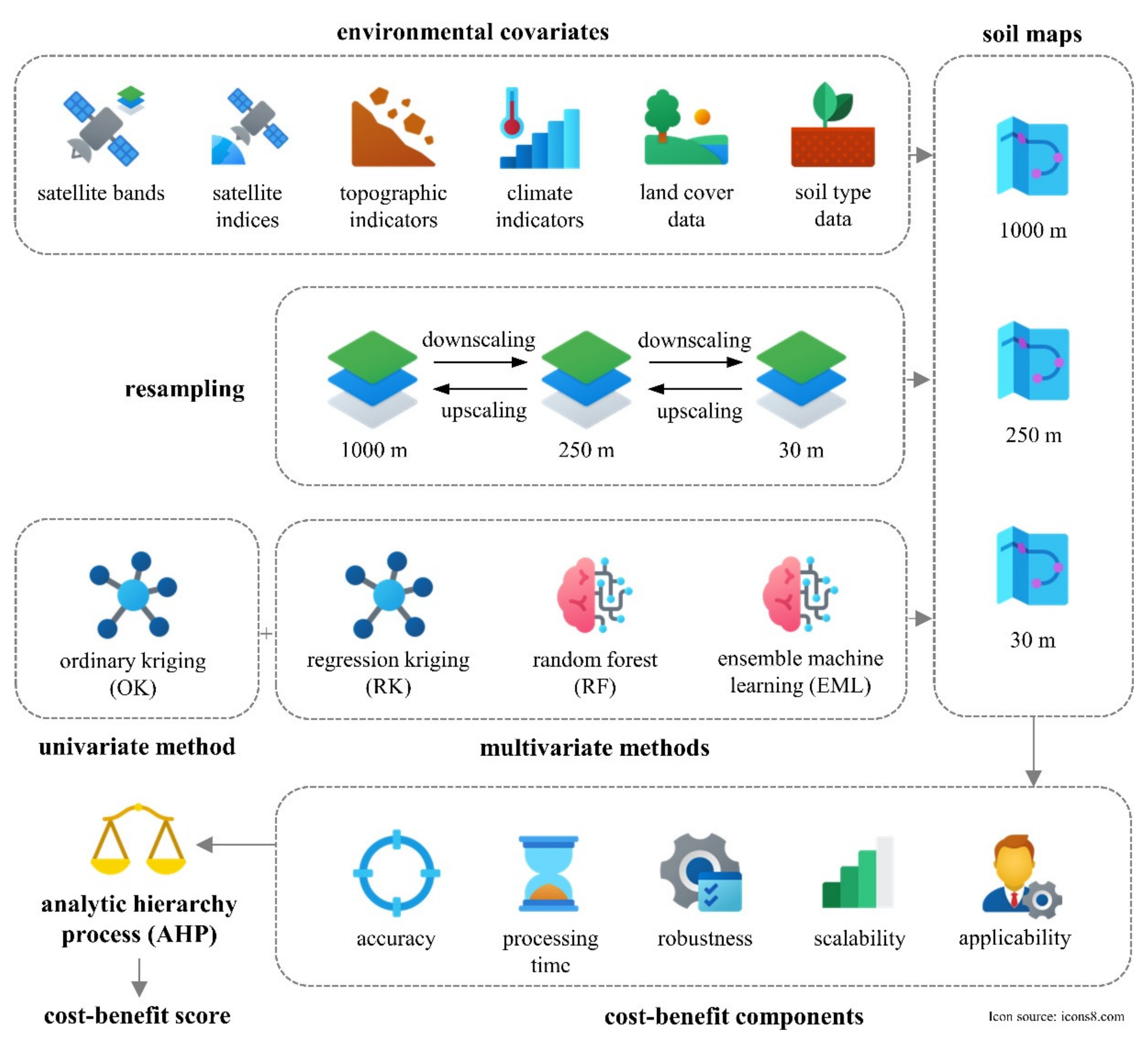
2. Materials and Methods

All spatial calculations were performed in the Croatian Terrestrial Reference System (HTRS96/TM) on three scales, which is official for the majority of scales in Croatia, including county level. Statistical, geostatistical and machine learning methods were performed using open-source software, including R x64 v4.0.3 in RStudio v2021.09.2 (Boston, MA, USA) for soil mapping and accuracy assessment, SAGA GIS v7.9.0 (Göttingen, Germany) for preprocessing of environmental covariates and QGIS v3.10 (Grüt, Switzerland) for visualization of spatial data. The workflow of the study is represented in Figure 1.
As a part of the cost–benefit analysis, soil mapping and accuracy assessment were performed independently using hardware with different computational possibilities. The first one was a custom GIS workstation with high potential computational efficiency, having the specifications of an Intel i9-9900X 3.50 GHz processor, 64.00 GB RAM and NVIDIA Quadro P4000 8.00 GB graphics processing unit. The second piece of hardware consisted of a serial-production laptop with an Intel i5-10300H 2.50 GHz processor, 8.00 GB RAM and NVIDIA GeForce GTX 1650 4.00 GB graphics processing unit. These options represented a more expensive (workstation) and a cheaper, widely available solution (laptop) to evaluate cost efficiency as a segment of the cost–benefit approach to digital soil mapping in addition to prediction accuracy assessment and computational efficiency.

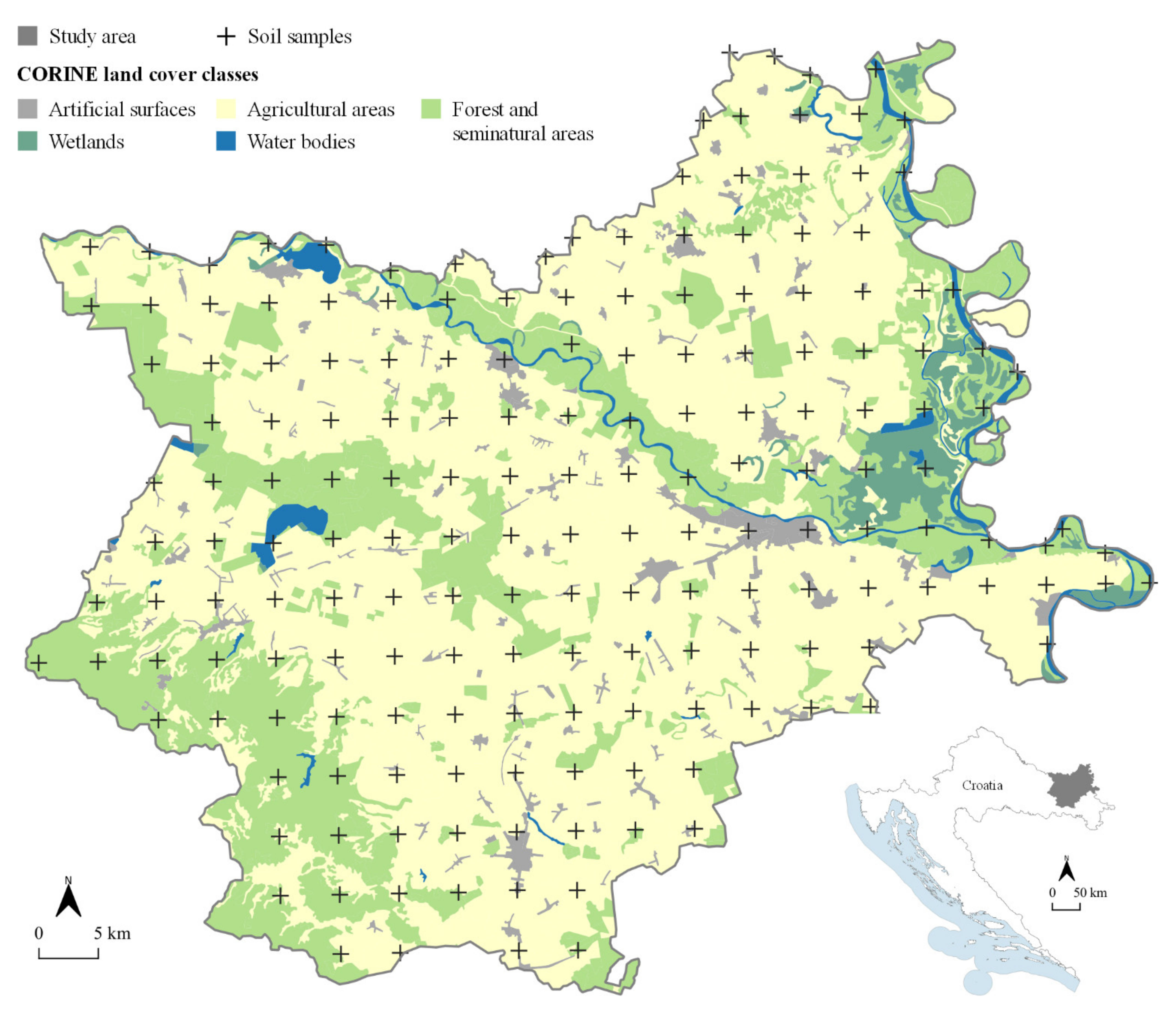
2.1. Study Area and Soil Sampling Data

The study area was the Osijek-Baranja county, a 4155 km2 area located in eastern Croatia (Figure 2). The agricultural area is the dominant land cover class per Coordinate Information on the Environment (CORINE) 2012 land cover data [42], covering 62.8% of the study area. It dominantly consists of arable cropland, which is mainly utilized for cereal production. Despite the traditionally agricultural character of the county, forests with seminatural areas (27.9%) and the wetland area of the Nature Park Kopački rit (3.7%) cause notable heterogeneity of land cover. These properties give it significance from the perspectives of agricultural production and nature protection, not only on a national but also on a regional scale [11]. A moist, subhumid climate, classified as “Cfwbx” on the Köppen scale, is present in the entire study area.
The 178 soil samples used in the study were collected using a regular grid sampling system. Soil samples were received from the results of the national scientific project performed between 2014 and 2017, available using the Web Feature Service (WFS) service of the former Croatian Agency for the Environment and Nature [43]. The fieldwork of the soil sampling was finished in the year 2013, consisting of total soil carbon (TC) and total soil nitrogen values (TN) at the 0–30 cm soil depth. With the exception of water bodies, all four primary land cover classes were represented in the soil sampling.

2.2. Spatial Interpolation and Prediction Methods

According to their frequency of use in previous studies in the scientific journals indexed in the Web of Science Core Collection over the past decade [14], and the relative superiority of prediction accuracy compared to contemporary methods [13,17,44], four prediction methods were evaluated in this study. These were two geostatistical (OK, RK) and two machine learning methods (RF, EML). Three R programming language packages were used for soil mapping using these methods: “gstat” for OK and RK [45], ”ranger” for RF [24] and “landmap” for EML [46].
OK is considered as the best linear, unbiased spatial predictor [47] and has been the most frequently used spatial interpolation method for the prediction of soil properties during the past decade in general [14]. Exponential, spherical, Gaussian and Bessel mathematical models were evaluated in the study, and the optimal one was determined with the criterion of the highest prediction accuracy in each individual instance. Predicted value using OK interpolation method at unknown location x 0 was determined by Equation (1) [15]:
z ( x 0 ) = I = 1 n I   ×   z I i ,
where λ i is weight at the sampled location x i based on the variogram, and z( x i ) is sampled soil TC and TN value. Its performance is conditioned by the properties of input soil samples, requiring the presence of positive spatial autocorrelation, normal distribution and stationarity of data [11]. Predicted values using the RK method were determined by Equation (2) [48]:
z ( x 0 ) = k = 0 p β ^ k   ×   q k x 0 + i = 1 n λ i   ×   e x i ,
where β ^ k is drift model coefficients, q k is values of environmental covariates and e( x i ) is the residual at the sampled location x i . This approach enabled more accurate prediction of soil properties than OK, and these two methods are generally fundamental in the conventional approach to soil mapping [49]. While RK consistently provided high prediction accuracy in previous studies and was successfully evaluated as a universal approach to soil mapping, its disadvantages, lower computational efficiency than OK and unstable performance in cases with a small number of input soil samples, remain a challenge [48].
The applied “landmap” package incorporated RF, SVM, extreme gradient boosting (“xgboost” package), feed-forward neural networks (“nnet” package) and generalized linear models with elastic net regularization regression methods (“cvglmnet” package) [46]. The early studies which incorporated this state-of-the-art approach noted its robustness and superior prediction accuracy compared to individual machine learning methods, but these were achieved at the expense of computational efficiency and the need for powerful hardware [6]. While they did not allow maximum computational efficiency, RF and EML prediction were performed in a single block, making the process of preprocessing straightforward and ensuring the suitability for the automation of the prediction.

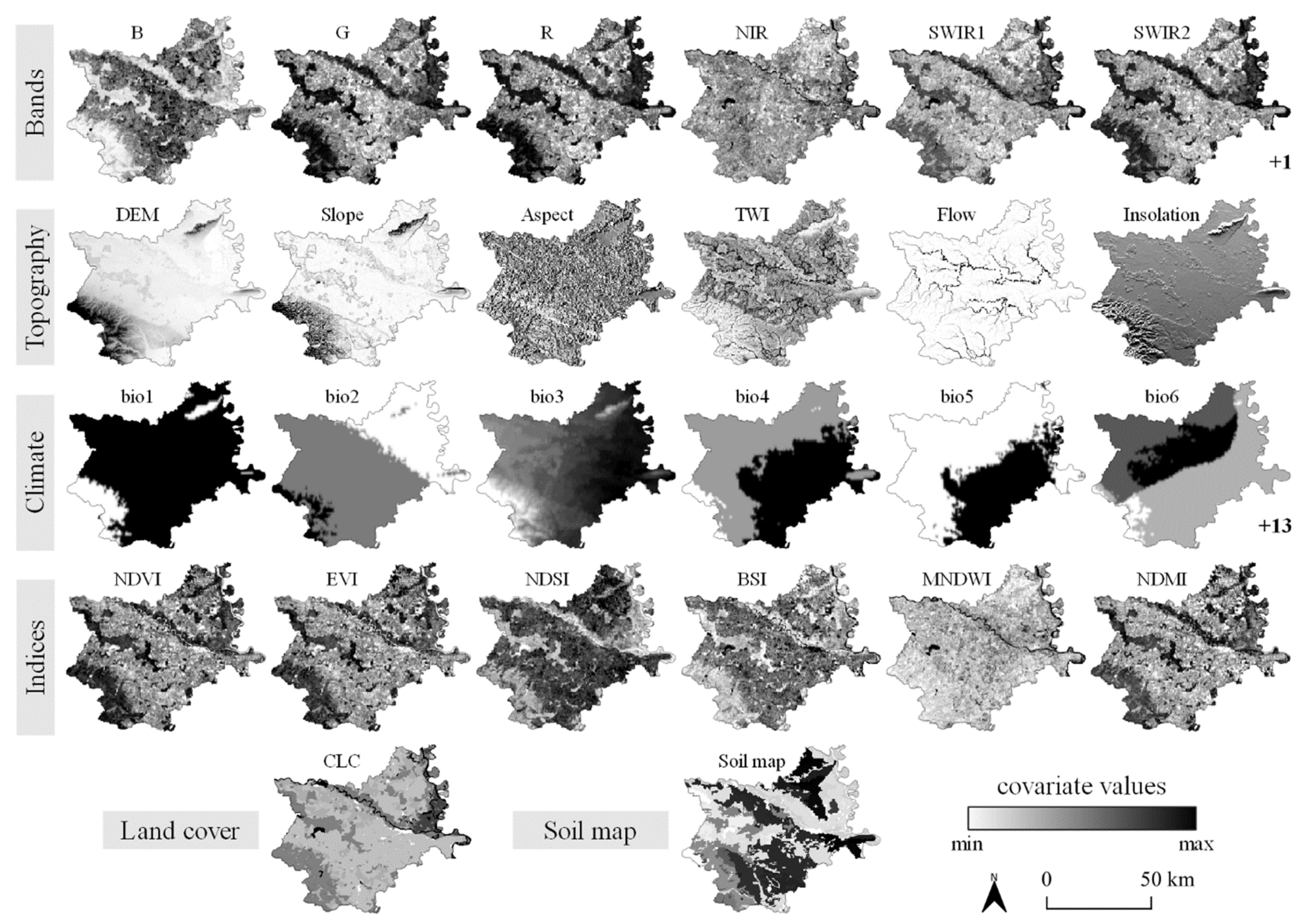
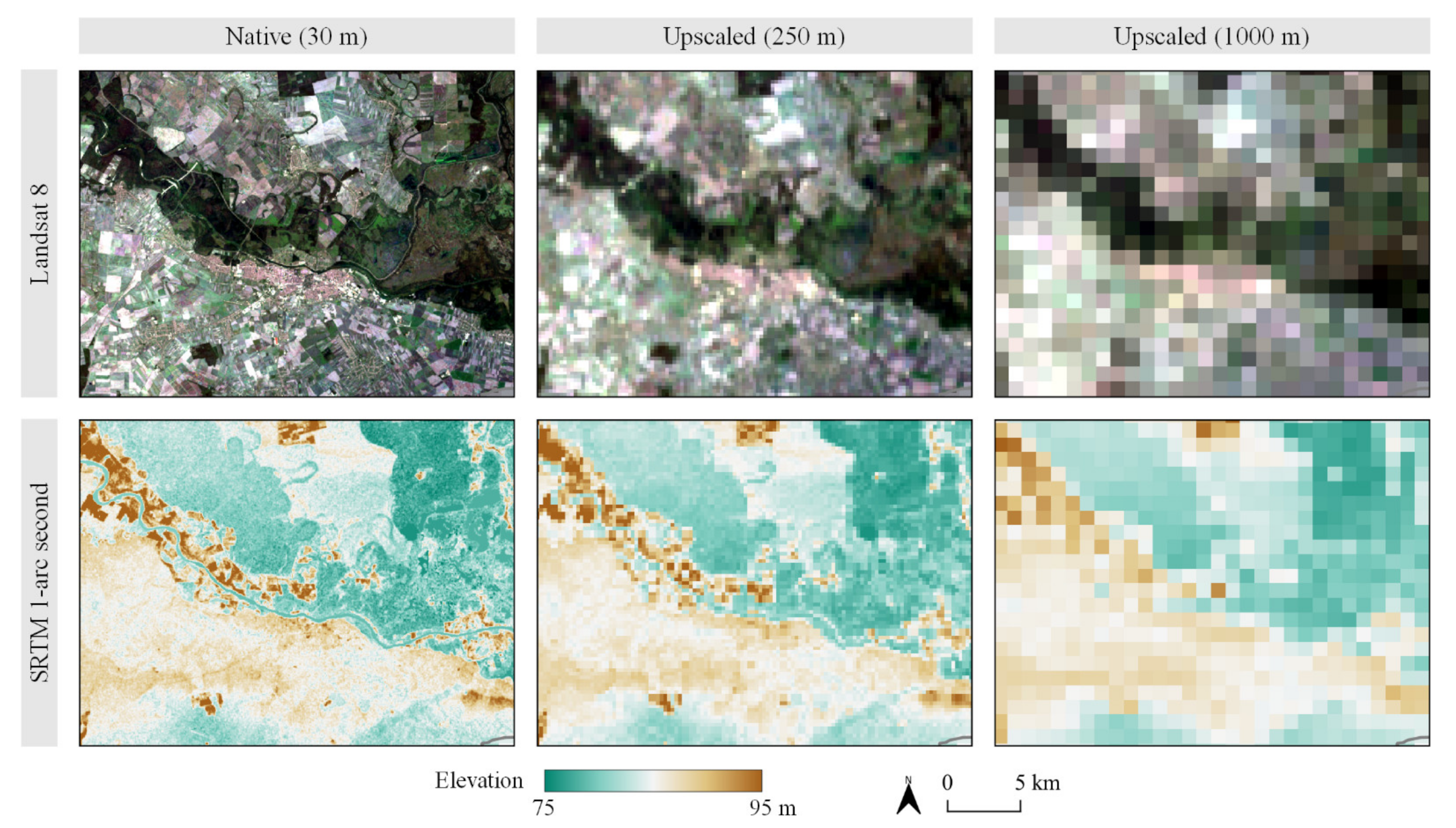
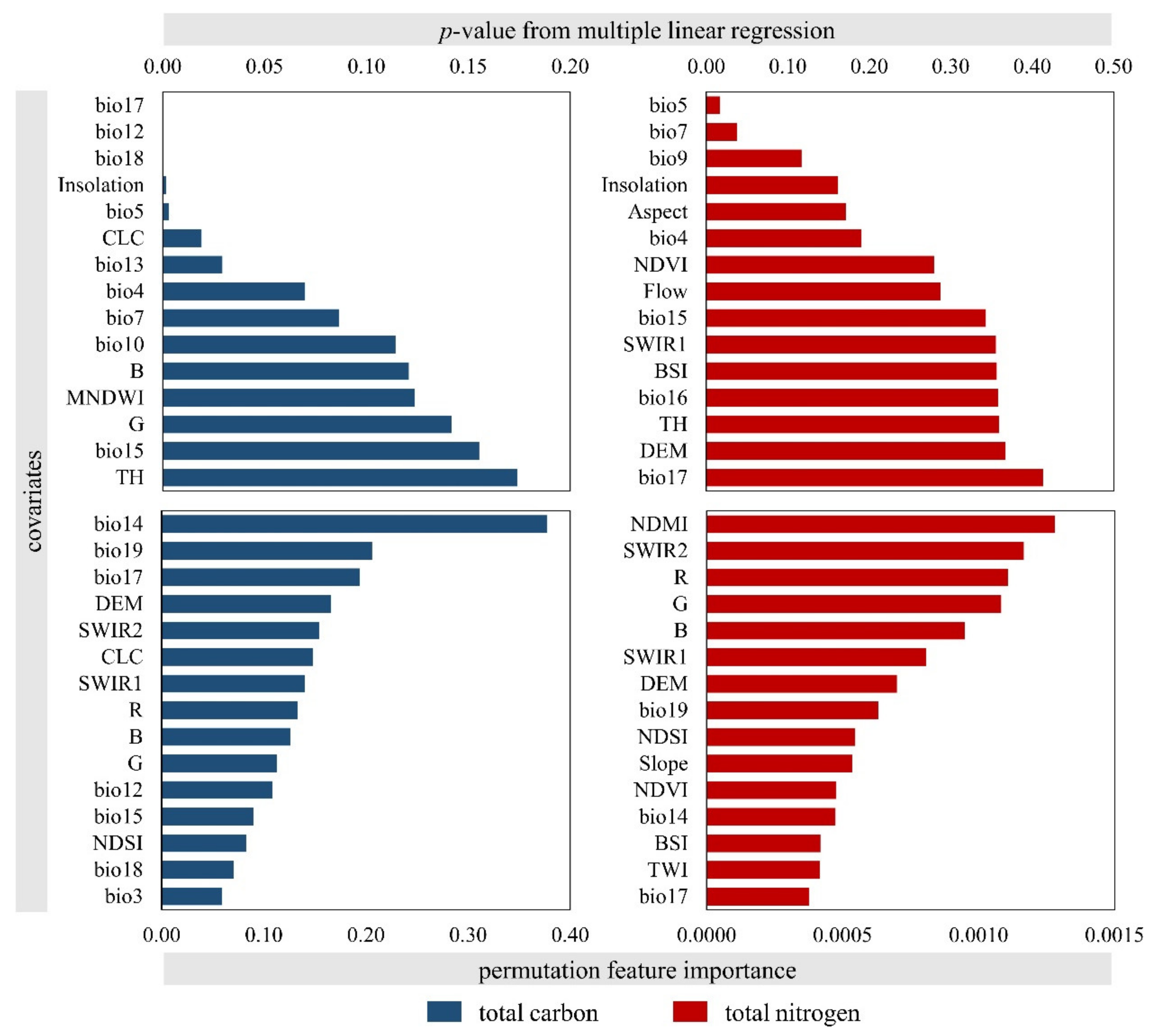
2.3. Environmental Covariates

Relevant environmental covariates for prediction of soil TC and TN included a variety of satellite remote sensing, climate, topography, land cover and auxiliary soil data. The individual layers used for environmental covariates for soil mapping in this study are displayed in Table 1, chosen according to the specifications of Hengl et al. [6,25,50] and Poggio et al. [51]. All environmental covariates were time-referenced to the soil sampling period, which was the year 2013. These environmental covariates are visualized in Figure 3.
Input environmental covariates were resampled to three datasets according to three spatial resolutions: (1) maximum of 30 m, according to the highest native spatial resolution of Landsat 8 multispectral imagery and SRTM 1 arc-second DEM; (2) optimum of 250 m, according to the inspection density method proposed by Hengl [55], with finest legible resolution from Equation (3); (3) minimum of 1000 m, according to the coarsest input spatial resolution of the CHELSA climate dataset.
optimal   resolution = 0 . 05   ×   A N  
where A is the study area, and N is the number of soil samples. Downscaling of the CHELSA climate dataset from the native 1000 m spatial resolution was performed using the B-spline interpolation method, which was determined as optimal for the same dataset and study area coverage [56]. For the environmental covariates with higher native spatial resolution, such as those from Landsat 8 (30 m) and SRTM 1 arc-second DEM (30 m) data, upscaling was performed with a weighted mean value calculation based on relative pixel area. A comparative display of Landsat 8 and SRTM 1 arc-second DEM data in native and upscaled spatial resolutions in the three created datasets is presented in Figure 4.

2.4. Cost–Benefit Analysis of Evaluated Soil Prediction Methods

As one of the most frequently used methods for multicriteria decision analysis, the analytical hierarchy process (AHP) is noted for its flexibility and straightforwardness in decision making [57,58]. The selected criteria included all major components of the soil prediction process, summarized in Table 2. The process of weight determination for individual criteria was based on the pairwise comparison matrix, which quantifies the relative importance of all possible combinations of selected criteria [59]. Relative importance was assessed by designating a number in the range between 1 and 9, proportionally quantifying importance from equally important to significantly more important. Consistency of the pairwise comparison was performed using the consistency ratio (CR) as a ratio of study-specific consistency index (CI) and predetermined random index (RI) [60]. CR values below 0.10 indicate consistent pairwise comparison. As the process of pairwise comparison is specific for each study area and dataset, observations from previous studies regarding land management and decision making related to digital soil mapping were used to reduce the subjectivity of the process [1,5,26,61].
To further reduce the subjectivity of the AHP process, a fully objective linear scaling method was adopted for the standardization of input values in the (0,1) number interval [62]. All input values per individual criterion were transformed to match 0 for the least favorable value x min and 1 for the most favorable value x max , while intermediate values x were calculated using Equation (4):
standardized   value = x     x min x max   x min .
The final cost–benefit suitability values were calculated using the weighted linear combination from the standardized values and respective weights from individual criteria. The possible value range matched those of the standardized values, ranging from 0 for the lowest to 1 for the highest.
The accuracy assessment from the geostatistical methods (OK, RK) was performed using cross-validation with the leave-one-out method, while machine learning (RF, EML) was evaluated using the out-of-bag (OOB) values. The statistical metrics used for the accuracy assessment were the coefficient of determination (R2) (Equation (5)), root-mean-square error (RMSE) (Equation (6)) and normalized RMSE (NRMSE) (Equation (7)). R2 and RMSE were traditionally used for the accuracy assessment of both geostatistical and machine learning methods in previous studies, enabling complementary evaluation of the average prediction accuracy [11,40]. By dividing RMSE by the mean of sampled values z ( x 0 ) ¯   , NRMSE provided a base for the mutual comparative assessment of TC and TN prediction due to their difference in value ranges.
R 2 = 1 1 n z ( x 0 )     z ( x i ) 2 1 n z ( x 0 )     z ( x 0 ) ¯   2 ,
RMSE   = 1 n ( z ( x 0 )     z ( x i ) ) 2 n ,
NRMSE = RMSE z ( x 0 ) ¯   ,
Measurements for processing times were performed under equal conditions for all instances of soil prediction. Total processing times were measured in ms, with the starting and ending point of the measurement being set right before and after the processed code of the particular prediction method, respectively. In addition to structuring the R script to include the minimal required amount of intermediate data for prediction, minor optimization steps were performed, including removal of obsolete intermediate data from the environment and minimization of memory usage by the garbage collection function.
Robustness and scalability were derived from the accuracy assessment results prior to the standardization. Robustness was quantified by deducting the top R2 values for the TC and TN of each prediction method, while scalability was determined by deducting the top R2 values of the 30 m/250 m results from those in 1000 m spatial resolution. The applicability criterion was subjectively estimated, with a value of 1 being designated for the univariate method with no covariates needed, 0.5 for the direct input of covariates and 0 in cases where covariates required additional analysis.

3. Results

Both sampled datasets were similar in that they did not possess normal distribution and had a moderate level of dispersion from their respective mean values (Table 3). The sole and highly notable difference between the TC and TN input sample sets was the degree of spatial autocorrelation expressed with Moran’s I. TC had a moderately high positive spatial autocorrelation, whereas TN indicated a very low degree. This is displayed in more detail in Figure 5, revealing the presence of positive autocorrelation for TC values up to 31,200 m distance, while autocorrelation values of TN remained consistently low in the entire search radius.

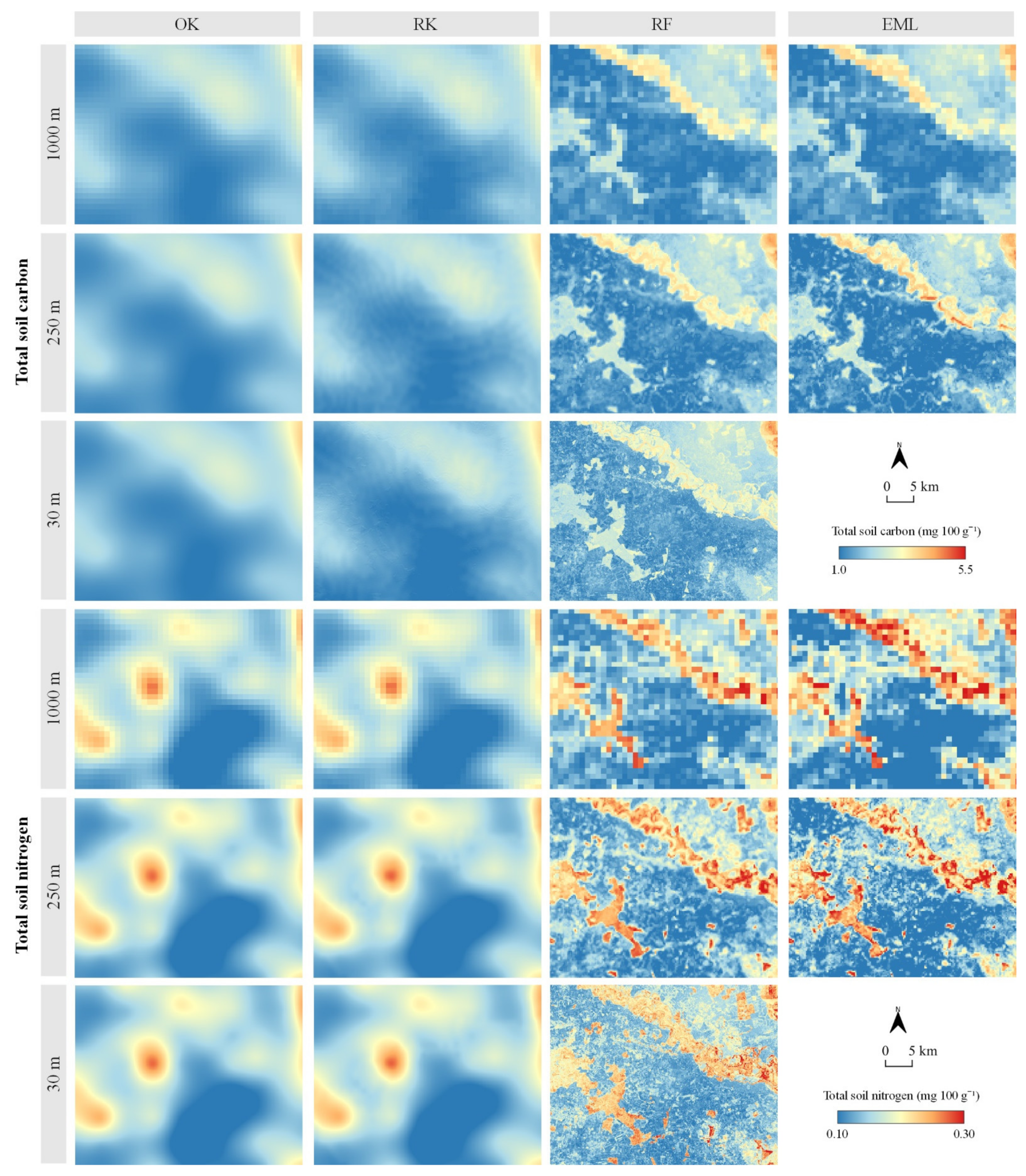
Predicted Soil TC and TN Values with Accuracy Assessment

Variogram parameters for TC (n = 0.666, s = 1.191, r = 9076 m) and TN (n = 0.003, s = 0.005, r = 4672 m) were equal for all three evaluated spatial resolutions of OK and RK interpolation. The Bessel mathematical model was determined as the most suitable for geostatistical prediction, achieving the highest prediction accuracy based on the iterative assessment of the mathematical models.
Accuracy assessment indicators for OK and RK were equal for all evaluated spatial resolutions and their respective soil parameters (Table 4). Machine learning methods achieved superior prediction accuracy compared to geostatistical methods in all evaluated instances. While OK and RK prediction accuracy noticeably dropped for low spatial autocorrelation TN data, RF and EML were more resistant to this property. RF produced very similar results between the spatial resolutions of respective soil parameters caused by randomness of the algorithm. EML benefited from the increased heterogeneity of environmental covariates and achieved higher spatial resolution. It produced the highest prediction accuracy for both soil TC and TN and was particularly superior to all evaluated methods, including RF for TN values.
Based on the statistical significance of environmental covariates from the multiple linear regression, insolation, bio12, bio17 and bio18, representing precipitation bioclimatic variables, had a 0.001 level of significance (Figure 6). Two other bioclimatic variables related to air temperature, bio5 and bio7, were significant to soil TN values with a 0.05 level. Top feature importance values for TC were in line with those from the multiple linear regression, with the precipitation covariates being the most impactful ones. The same values for TN adopted a notably lower value range, with spectral bands and indices derived from Landsat 8 data having the highest importance.
While RF was a part of EML, it did not produce statistically significant results for either soil property. For TC, cvglmnet and SVM resulted in statistically significant results, while nnet produced the same for TN. EML prediction of both soil TC and TN could not be performed due to hardware limitations. A multiscale comparative visual display of predicted soil TC and TN for the subset of study area is presented in Figure 7.
Resulting processing times showed the same exponential grow for both the workstation and laptop proportional to the number of pixels for prediction, resulting in notably higher values for the 30 m spatial resolution (Table 5). RF was the most computationally efficient prediction method of all the evaluated iterations. The workstation required 8.1% less processing time for OK prediction, 4.0% less for RK, 15.5% less for RF and 1.8% less for EML than the laptop. In addition to the minor computational superiority of the workstation, it also enabled RF prediction at 30 m spatial resolution, which could not be processed using the laptop due to memory shortage.
The pairwise comparison matrix within the cost–benefit analysis using AHP is displayed in Table 6. The prediction accuracy resulted in the highest individual criteria weight, representing almost half of the impact on cost–benefit score, followed by processing time and robustness (Table 7). With the maximum standardized values in accuracy, robustness and scalability, EML resulted in the highest cost–benefit score. RF was the second-ranked method, having a 36% lower cost–benefit score than EML despite being the superior method regarding computational efficiency. Both geostatistical methods (OK and RK) ranked below machine learning methods and had similar standardized values, with the main difference in the applicability values being due to the univariate property of OK.

4. Discussion

While previous research focused primarily on the prediction accuracy component of soil mapping, this study additionally integrated an evaluation of processing time, robustness, scalability and applicability into a cost–benefit analysis. Based on the value range and distribution, evaluated TC and TN soil sample data represented two very distinct cases of input values for soil mapping. While the absence of input data normality is usually negated by introducing the logarithmic transformation [63], as was the case for TC, the additional lack of spatial autocorrelation for TN disabled the accurate kriging interpolation. This property was also a frequent occurrence in previous studies [64,65,66], indicating the necessity of a framework that does not require such prerequisites. Since value distributions of TC and TN represent a highly common case, a universal approach to soil prediction should be resistant to these properties, a criterion which was not met by the OK and RK geostatistical approaches in this study. In addition to its superior prediction accuracy compared to other evaluated methods, EML proved resistant to the properties of input values, as well as the scalability of prediction. Mishra et al. [20] confirmed the superior prediction accuracy of EML compared to individual machine learning methods and RK for the prediction of soil organic carbon at the 250 m spatial resolution. This also proved the robustness of both EML and individual machine learning methods regarding the level of generalization of input environmental covariates. The same authors adopted broad and generalized covariates, contrary to more numerous, specific monthly and bioclimatic data related to air temperature and precipitation in this study. By comparing the R2 and RMSE of this study, EML and RF likely benefited from the more specific covariates, achieving higher accuracy relative to the geostatistical approach. Additionally, Baltensweiler et al. [38] successfully integrated multiple data sources of a single environmental component in the case of unknown adequacy for soil mapping. Gavilán-Acuña et al. [67] reached similar conclusions regarding EML’s superiority to individual geostatistical and machine learning methods in forestry, with a larger relative accuracy of OK and RK methods. Despite convincingly achieving the highest cost–benefit score, the very high computational demand of EML currently prevents its automation within soil mapping frameworks and widespread application on a larger scale. In such cases, RF performs as a solid alternative, ensuring high prediction accuracy with a moderate cost–benefit score. Moreover, Nussbaum et al. [39] noted that, while EML mainly ensures higher prediction accuracy, RF can produce superior results for some soil parameters, achieving the lowest cost–benefit score of the geostatistical OK and RK methods, which indicates their obsoleteness in the face of machine learning methods. Despite relatively subpar performance, OK remains the most represented soil prediction method in scientific studies [14], ensuring high applicability and simplicity due to its univariate property, as well as user-friendly implementation in widely used GIS software, such as ArcGIS and SAGA GIS [68]. In cases of missing, adequate environmental covariates, a univariate approach based on RF was developed by Hengl et al. [40], which resolves the single disadvantage of the machine learning approach in geostatistics, which relates to its applicability.
Further improvement of the cost–benefit evaluation approach regarding the methods used for prediction of soil properties should be directed towards the three disadvantages of the proposed approach:
  • As was the case in various applications of AHP in previous suitability and decision-making studies [69], the process of pairwise comparison was almost entirely subjective. While this property can be mitigated by the application of the objective, deterministic approach of the linear scaling standardization method, final cost–benefit values are still, to some degree, affected by the subjectivity of the user. An unsupervised classification of the cost–benefit components might be a more suitable solution for objective assessment, but the ranking of classes still has to be performed according to arbitrary, subjective criteria [11]. Nevertheless, the subjective component of the AHP could also be an advantage due to its flexibility relating to the needs of the specific study area and demands from a decision-making standpoint;
  • Further optimization of the prediction process for the soil mapping in 30 m spatial resolution can be performed. This was successfully solved by prediction in blocks [46], but this approach prevents full automation of the procedure or includes further complexity of the prediction. In addition to RF, SVM, xgboost, nnet and cvglmnet implemented in the “landmap” package for EML, the addition of methods, such as RK [20] or geoadditive modeling and cubist [38], could ensure additional accuracy and robustness of the EML;
  • Downscaling of the environmental covariates with lower native spatial resolution than 30 m inevitably includes a degree of data interpolation. While this approach could reduce the reliability of input data, downscaled data might actually be slightly more accurate when compared to the ground-truth data than those in native resolution [56]. For a more robust approach, negating the effects of downscaling, a two-scale EML approach is potentially more suitable [46]. In addition to soil mapping, this approach could enable accurate prediction of similar spatial components of the environment, such as erosion susceptibility [58], cropland suitability [56] and habitats of endangered flora species, in high spatial resolution.

5. Conclusions

This study added an additional perspective on the specific properties of the most frequently used geostatistical and machine learning methods, building on the emphasis given to prediction accuracy in previous studies. This comprehensive approach to the evaluation of soil prediction methods included five cost–benefit criteria in AHP evaluation: accuracy, processing time, robustness, scalability and applicability. In addition to conventional, strict focus on prediction accuracy, this approach provided an in-depth performance evaluation, considering the time consumption and applicability of soil mapping methods for land management experts. With respect to previous studies and the native spatial resolutions of main data sources for environmental covariates, the multiscale approach of this study consisted of soil prediction at 1000 m, 250 m and 30 m.
The cost–benefit analysis suggested that EML is a superior prediction method compared to geostatistics and individual machine learning methods regarding prediction accuracy, robustness and scalability. While computational efficiency impaired its cost–benefit value, further optimization of EML algorithms and improved computer hardware could ensure its wider applicability in the future. The prediction of soil properties using EML presently supports spatial resolutions up to about a few hundred meters over a county-level area using a widely available hardware for land management experts. This indicates that the primary focus of upgrading EML packages should be increasing computational efficiency. While this can be resolved by prediction in blocks, at this point, the required processing time remains its largest disadvantage and prevents widespread use. RF performed as its best alternative, especially as it has the lowest necessary processing time, while retaining high prediction accuracy. With only a slightly lower prediction accuracy than EML, RF could presently be the optimal prediction method for soil mapping at about 30 m spatial resolution for a large number of study areas and datasets. Geostatistical methods, OK and RK, were obsolete in most of the evaluated cost–benefit components in the face of machine learning methods, despite their popularity in recent scientific studies. According to the criteria for the cost–benefit analysis in this study, machine learning prediction methods for soil mapping overtook the performance of conventional methods, with the sole disadvantage being a lack of environmental covariates for the prediction. A paradigm shift towards the machine learning approach in soil mapping has emerged in recent years largely for this reason, and its further propagation is expected in the near future, primarily in relation to increasing the computational efficiency of available software packages for prediction.

Author Contributions

Conceptualization, D.R.; methodology, D.R.; software, D.R.; validation, D.R., M.J., O.A., A.Š., N.C., I.R., I.P. and M.G.; formal analysis, D.R. and M.G.; investigation, D.R.; resources, D.R.; data curation, D.R.; writing—original draft preparation, D.R. and M.G.; writing—review and editing, D.R., M.J., O.A., A.Š., N.C., I.R., I.P. and M.G.; visualization, D.R.; supervision, M.J., O.A., A.Š., N.C., I.R., I.P. and M.G. project administration, M.J.; funding acquisition, M.J. All authors have read and agreed to the published version of the manuscript.

Funding

This research received no external funding.

Institutional Review Board Statement

Not applicable.

Informed Consent Statement

Not applicable.

Data Availability Statement

Not applicable.

Acknowledgments

This work was supported by the Faculty of Agrobiotechnical Sciences Osijek as a part of the scientific project “AgroGIT—technical and technological crop production systems, GIS and environment protection”.

Conflicts of Interest

The authors declare no conflict of interest.

References

  1. Cabrini, S.M.; Calcaterra, C.P. Modeling Economic-Environmental Decision Making for Agricultural Land Use in Argentinean Pampas. Agric. Syst. 2016, 143, 183–194. [Google Scholar] [CrossRef]
  2. Ellison, D.; Morris, C.E.; Locatelli, B.; Sheil, D.; Cohen, J.; Murdiyarso, D.; Gutierrez, V.; van Noordwijk, M.; Creed, I.F.; Pokorny, J.; et al. Trees, Forests and Water: Cool Insights for a Hot World. Glob. Environ. Change 2017, 43, 51–61. [Google Scholar] [CrossRef]
  3. Radočaj, D.; Jurišić, M.; Gašparović, M. A Wildfire Growth Prediction and Evaluation Approach Using Landsat and MODIS Data. J. Environ. Manag. 2022, 304, 114351. [Google Scholar] [CrossRef]
  4. Pelorosso, R.; Gobattoni, F.; Geri, F.; Monaco, R.; Leone, A. Evaluation of Ecosystem Services Related to Bio-Energy Landscape Connectivity (BELC) for Land Use Decision Making across Different Planning Scales. Ecol. Indic. 2016, 61, 114–129. [Google Scholar] [CrossRef]
  5. Minasny, B.; McBratney, A.B. Digital Soil Mapping: A Brief History and Some Lessons. Geoderma 2016, 264, 301–311. [Google Scholar] [CrossRef]
  6. Hengl, T.; de Jesus, J.M.; Heuvelink, G.B.M.; Gonzalez, M.R.; Kilibarda, M.; Blagotić, A.; Shangguan, W.; Wright, M.N.; Geng, X.; Bauer-Marschallinger, B.; et al. SoilGrids250m: Global Gridded Soil Information Based on Machine Learning. PLoS ONE 2017, 12, e0169748. [Google Scholar] [CrossRef]
  7. McBratney, A.B.; Mendonça Santos, M.L.; Minasny, B. On Digital Soil Mapping. Geoderma 2003, 117, 3–52. [Google Scholar] [CrossRef]
  8. Meena, V.S.; Mondal, T.; Pandey, B.M.; Mukherjee, A.; Yadav, R.P.; Choudhary, M.; Singh, S.; Bisht, J.K.; Pattanayak, A. Land Use Changes: Strategies to Improve Soil Carbon and Nitrogen Storage Pattern in the Mid-Himalaya Ecosystem, India. Geoderma 2018, 321, 69–78. [Google Scholar] [CrossRef]
  9. Pellegrini, A.F.A.; Ahlström, A.; Hobbie, S.E.; Reich, P.B.; Nieradzik, L.P.; Staver, A.C.; Scharenbroch, B.C.; Jumpponen, A.; Anderegg, W.R.L.; Randerson, J.T.; et al. Fire Frequency Drives Decadal Changes in Soil Carbon and Nitrogen and Ecosystem Productivity. Nature 2018, 553, 194–198. [Google Scholar] [CrossRef] [PubMed]
  10. Yu, Q.; Hu, X.; Ma, J.; Ye, J.; Sun, W.; Wang, Q.; Lin, H. Effects of Long-Term Organic Material Applications on Soil Carbon and Nitrogen Fractions in Paddy Fields. Soil Tillage Res. 2020, 196, 104483. [Google Scholar] [CrossRef]
  11. Radočaj, D.; Jurišić, M.; Antonić, O. Determination of Soil C:N Suitability Zones for Organic Farming Using an Unsupervised Classification in Eastern Croatia. Ecol. Indic. 2021, 123, 107382. [Google Scholar] [CrossRef]
  12. Hengl, T.; Heuvelink, G.B.M.; Stein, A. A Generic Framework for Spatial Prediction of Soil Variables Based on Regression-Kriging. Geoderma 2004, 120, 75–93. [Google Scholar] [CrossRef]
  13. Shen, Q.; Wang, Y.; Wang, X.; Liu, X.; Zhang, X.; Zhang, S. Comparing Interpolation Methods to Predict Soil Total Phosphorus in the Mollisol Area of Northeast China. Catena 2019, 174, 59–72. [Google Scholar] [CrossRef]
  14. Radočaj, D.; Jurišić, M.; Gašparović, M. The Role of Remote Sensing Data and Methods in a Modern Approach to Fertilization in Precision Agriculture. Remote Sens. 2022, 14, 778. [Google Scholar] [CrossRef]
  15. Oliver, M.A.; Webster, R. A Tutorial Guide to Geostatistics: Computing and Modelling Variograms and Kriging. Catena 2014, 113, 56–69. [Google Scholar] [CrossRef]
  16. Bogunovic, I.; Kisic, I.; Mesic, M.; Percin, A.; Zgorelec, Z.; Bilandžija, D.; Jonjic, A.; Pereira, P. Reducing Sampling Intensity in Order to Investigate Spatial Variability of Soil PH, Organic Matter and Available Phosphorus Using Co-Kriging Techniques. A Case Study of Acid Soils in Eastern Croatia. Arch. Agron. Soil Sci. 2017, 63, 1852–1863. [Google Scholar] [CrossRef]
  17. Gia Pham, T.; Kappas, M.; Van Huynh, C.; Hoang Khanh Nguyen, L. Application of Ordinary Kriging and Regression Kriging Method for Soil Properties Mapping in Hilly Region of Central Vietnam. ISPRS Int. J. Geo Inf. 2019, 8, 147. [Google Scholar] [CrossRef]
  18. Radočaj, D.; Jug, I.; Vukadinović, V.; Jurišić, M.; Gašparović, M. The Effect of Soil Sampling Density and Spatial Autocorrelation on Interpolation Accuracy of Chemical Soil Properties in Arable Cropland. Agronomy 2021, 11, 2430. [Google Scholar] [CrossRef]
  19. Li, J.; Heap, A.D. A Review of Spatial Interpolation Methods for Environmental Scientists. Geoscience: Canberra, Australia, 2008. [Google Scholar]
  20. Mishra, U.; Gautam, S.; Riley, W.J.; Hoffman, F.M. Ensemble Machine Learning Approach Improves Predicted Spatial Variation of Surface Soil Organic Carbon Stocks in Data-Limited Northern Circumpolar Region. Front. Big Data 2020, 3, 528441. [Google Scholar] [CrossRef] [PubMed]
  21. Song, J.J.; Kwon, S.; Lee, G. Incorporation of Parameter Uncertainty into Spatial Interpolation Using Bayesian Trans-Gaussian Kriging. Adv. Atmos. Sci. 2015, 32, 413–423. [Google Scholar] [CrossRef]
  22. Sahu, B.; Ghosh, A.K. Seema Deterministic and Geostatistical Models for Predicting Soil Organic Carbon in a 60 Ha Farm on Inceptisol in Varanasi, India. Geoderma Reg. 2021, 26, e00413. [Google Scholar] [CrossRef]
  23. Kuhn, M.; Wing, J.; Weston, S.; Williams, A.; Keefer, C.; Engelhardt, A.; Cooper, T.; Mayer, Z.; Kenkel, B.; R Core Team. Package ‘caret’. R J. 2020, 223, 7. [Google Scholar]
  24. Wright, M.N.; Ziegler, A. Ranger: A Fast Implementation of Random Forests for High Dimensional Data in C++ and R. arXiv 2015, arXiv:150804409. [Google Scholar] [CrossRef]
  25. Hengl, T.; de Jesus, J.M.; MacMillan, R.A.; Batjes, N.H.; Heuvelink, G.B.M.; Ribeiro, E.; Samuel-Rosa, A.; Kempen, B.; Leenaars, J.G.B.; Walsh, M.G.; et al. SoilGrids1km—Global Soil Information Based on Automated Mapping. PLoS ONE 2014, 9, e105992. [Google Scholar] [CrossRef]
  26. Chen, S.; Arrouays, D.; Leatitia Mulder, V.; Poggio, L.; Minasny, B.; Roudier, P.; Libohova, Z.; Lagacherie, P.; Shi, Z.; Hannam, J.; et al. Digital Mapping of GlobalSoilMap Soil Properties at a Broad Scale: A Review. Geoderma 2022, 409, 115567. [Google Scholar] [CrossRef]
  27. User Guides-Sentinel-2 MSI-Sentinel Online-Sentinel Online. Available online: https://sentinel.esa.int/web/sentinel/user-guides/sentinel-2-msi (accessed on 10 September 2022).
  28. Landsat 8 Data Users Handbook|U.S. Geological Survey. Available online: https://www.usgs.gov/media/files/landsat-8-data-users-handbook (accessed on 10 September 2022).
  29. User Guides-Sentinel-1 SAR-Sentinel Online-Sentinel Online. Available online: https://sentinel.esa.int/web/sentinel/user-guides/sentinel-1-sar (accessed on 10 September 2022).
  30. User Guides-Sentinel-3 OLCI-Sentinel Online-Sentinel Online. Available online: https://sentinel.esa.int/web/sentinel/user-guides/sentinel-3-olci (accessed on 10 September 2022).
  31. Landsat 9 Data Users Handbook|U.S. Geological Survey. Available online: https://www.usgs.gov/media/files/landsat-9-data-users-handbook (accessed on 10 September 2022).
  32. Karger, D.N.; Conrad, O.; Böhner, J.; Kawohl, T.; Kreft, H.; Soria-Auza, R.W.; Zimmermann, N.E.; Linder, H.P.; Kessler, M. Climatologies at High Resolution for the Earth’s Land Surface Areas. Sci. Data 2017, 4, 170122. [Google Scholar] [CrossRef]
  33. Fick, S.E.; Hijmans, R.J. WorldClim 2: New 1-Km Spatial Resolution Climate Surfaces for Global Land Areas. Int. J. Climatol. 2017, 37, 4302–4315. [Google Scholar] [CrossRef]
  34. EU-DEM v1.1—Copernicus Land Monitoring Service. Available online: https://land.copernicus.eu/imagery-in-situ/eu-dem/eu-dem-v1.1 (accessed on 21 April 2021).
  35. Wulder, M.A.; Loveland, T.R.; Roy, D.P.; Crawford, C.J.; Masek, J.G.; Woodcock, C.E.; Allen, R.G.; Anderson, M.C.; Belward, A.S.; Cohen, W.B.; et al. Current Status of Landsat Program, Science, and Applications. Remote Sens. Environ. 2019, 225, 127–147. [Google Scholar] [CrossRef]
  36. Phiri, D.; Simwanda, M.; Salekin, S.; Nyirenda, V.R.; Murayama, Y.; Ranagalage, M. Sentinel-2 Data for Land Cover/Use Mapping: A Review. Remote Sens. 2020, 12, 2291. [Google Scholar] [CrossRef]
  37. Breiman, L. Random Forests. Mach. Learn. 2001, 45, 5–32. [Google Scholar] [CrossRef]
  38. Baltensweiler, A.; Walthert, L.; Hanewinkel, M.; Zimmermann, S.; Nussbaum, M. Machine Learning Based Soil Maps for a Wide Range of Soil Properties for the Forested Area of Switzerland. Geoderma Reg. 2021, 27, e00437. [Google Scholar] [CrossRef]
  39. Nussbaum, M.; Spiess, K.; Baltensweiler, A.; Grob, U.; Keller, A.; Greiner, L.; Schaepman, M.E.; Papritz, A. Evaluation of Digital Soil Mapping Approaches with Large Sets of Environmental Covariates. SOIL 2018, 4, 1–22. [Google Scholar] [CrossRef]
  40. Hengl, T.; Nussbaum, M.; Wright, M.N.; Heuvelink, G.B.M.; Gräler, B. Random Forest as a Generic Framework for Predictive Modeling of Spatial and Spatio-Temporal Variables. PeerJ 2018, 6, e5518. [Google Scholar] [CrossRef]
  41. Belgiu, M.; Dragut, L. Random Forest in Remote Sensing: A Review of Applications and Future Directions. Isprs J. Photogramm. Remote Sens. 2016, 114, 24–31. [Google Scholar] [CrossRef]
  42. CORINE Land Cover User Manual. Available online: https://land.copernicus.eu/user-corner/technical-library/clc-product-user-manual (accessed on 10 September 2022).
  43. Data Europa, 2021. Changes in Soil Carbon Stocks and Calculation of Trends in Total Nitrogen and Organic Carbon in Soil and C: N Ratios. Available online: Https://Data.Europa.Eu/Data/Datasets/Zaliha-Ugljika-u-Tlu-Izracun-Trendova-Ukupnog-Dusika-i-Organskog-Ugljika-Te-Odnosa-c-n?Locale=en (accessed on 16 February 2022).
  44. Attorre, F.; Alfo, M.; De Sanctis, M.; Francesconi, F.; Bruno, F. Comparison of Interpolation Methods for Mapping Climatic and Bioclimatic Variables at Regional Scale. Int. J. Climatol. 2007, 27, 1825–1843. [Google Scholar] [CrossRef]
  45. Pebesma, E.J. Multivariable Geostatistics in S: The Gstat Package. Comput. Geosci. 2004, 30, 683–691. [Google Scholar] [CrossRef]
  46. Hengl, T.; Miller, M.A.E.; Križan, J.; Shepherd, K.D.; Sila, A.; Kilibarda, M.; Antonijević, O.; Glušica, L.; Dobermann, A.; Haefele, S.M.; et al. African Soil Properties and Nutrients Mapped at 30 m Spatial Resolution Using Two-Scale Ensemble Machine Learning. Sci. Rep. 2021, 11, 6130. [Google Scholar] [CrossRef]
  47. Seo, D.-J. Conditional Bias-Penalized Kriging (CBPK). Stoch. Environ. Res. Risk Assess. 2013, 27, 43–58. [Google Scholar] [CrossRef]
  48. Hengl, T.; Heuvelink, G.B.M.; Rossiter, D.G. About Regression-Kriging: From Equations to Case Studies. Comput. Geosci. 2007, 33, 1301–1315. [Google Scholar] [CrossRef]
  49. Santra, P.; Das, B.S.; Chakravarty, D. Spatial Prediction of Soil Properties in a Watershed Scale through Maximum Likelihood Approach. Environ. Earth Sci. 2012, 65, 2051–2061. [Google Scholar] [CrossRef]
  50. Hengl, T.; MacMillan, R.A. Predictive Soil Mapping with R; Lulu.com: Morrisville, NC, USA, 2019; ISBN 978-0-359-30635-0. [Google Scholar]
  51. Poggio, L.; de Sousa, L.M.; Batjes, N.H.; Heuvelink, G.B.M.; Kempen, B.; Ribeiro, E.; Rossiter, D. SoilGrids 2.0: Producing Soil Information for the Globe with Quantified Spatial Uncertainty. SOIL 2021, 7, 217–240. [Google Scholar] [CrossRef]
  52. Roy, D.P.; Wulder, M.A.; Loveland, T.R.; Woodcock, C.E.; Allen, R.G.; Anderson, M.C.; Helder, D.; Irons, J.R.; Johnson, D.M.; Kennedy, R.; et al. Landsat-8: Science and Product Vision for Terrestrial Global Change Research. Remote Sens. Environ. 2014, 145, 154–172. [Google Scholar] [CrossRef]
  53. Farr, T.G.; Rosen, P.A.; Caro, E.; Crippen, R.; Duren, R.; Hensley, S.; Kobrick, M.; Paller, M.; Rodriguez, E.; Roth, L.; et al. The Shuttle Radar Topography Mission. Rev. Geophys. 2007, 45. [Google Scholar] [CrossRef]
  54. Büttner, G. CORINE Land Cover and Land Cover Change Products. In Land Use and Land Cover Mapping in Europe: Practices & Trends; Manakos, I., Braun, M., Eds.; Remote Sensing and Digital Image Processing; Springer: Dordrecht, The Netherlands, 2014; pp. 55–74. ISBN 978-94-007-7969-3. [Google Scholar]
  55. Hengl, T. Finding the Right Pixel Size. Comput. Geosci. 2006, 32, 1283–1298. [Google Scholar] [CrossRef]
  56. Radočaj, D.; Jurišić, M.; Gašparović, M.; Plaščak, I.; Antonić, O. Cropland Suitability Assessment Using Satellite-Based Biophysical Vegetation Properties and Machine Learning. Agronomy 2021, 11, 1620. [Google Scholar] [CrossRef]
  57. Dedeoğlu, M.; Dengiz, O. Generating of Land Suitability Index for Wheat with Hybrid System Aproach Using AHP and GIS. Comput. Electron. Agric. 2019, 167, 105062. [Google Scholar] [CrossRef]
  58. Domazetović, F.; Šiljeg, A.; Lončar, N.; Marić, I. Development of Automated Multicriteria GIS Analysis of Gully Erosion Susceptibility. Appl. Geogr. 2019, 112, 102083. [Google Scholar] [CrossRef]
  59. Saaty, T.L. Decision Making with the Analytic Hierarchy Process. Int. J. Serv. Sci. 2008, 1, 83–98. [Google Scholar] [CrossRef]
  60. Saaty, T.L.; Ozdemir, M.S. Why the Magic Number Seven plus or Minus Two. Math. Comput. Model. 2003, 38, 233–244. [Google Scholar] [CrossRef]
  61. Dong, W.; Wu, T.; Luo, J.; Sun, Y.; Xia, L. Land Parcel-Based Digital Soil Mapping of Soil Nutrient Properties in an Alluvial-Diluvia Plain Agricultural Area in China. Geoderma 2019, 340, 234–248. [Google Scholar] [CrossRef]
  62. Radočaj, D.; Jurišić, M.; Gašparović, M.; Plaščak, I. Optimal Soybean (Glycine Max L.) Land Suitability Using GIS-Based Multicriteria Analysis and Sentinel-2 Multitemporal Images. Remote Sens. 2020, 12, 1463. [Google Scholar] [CrossRef]
  63. Panday, D.; Maharjan, B.; Chalise, D.; Shrestha, R.K.; Twanabasu, B. Digital Soil Mapping in the Bara District of Nepal Using Kriging Tool in ArcGIS. PLoS ONE 2018, 13, e0206350. [Google Scholar] [CrossRef]
  64. Meng, Y.; Cave, M.; Zhang, C. Comparison of Methods for Addressing the Point-to-Area Data Transformation to Make Data Suitable for Environmental, Health and Socio-Economic Studies. Sci. Total Environ. 2019, 689, 797–807. [Google Scholar] [CrossRef]
  65. Fu, C.; Zhang, H.; Tu, C.; Li, L.; Luo, Y. Geostatistical Interpolation of Available Copper in Orchard Soil as Influenced by Planting Duration. Environ. Sci. Pollut. Res. 2018, 25, 52–63. [Google Scholar] [CrossRef]
  66. Mondejar, J.P.; Tongco, A.F. Estimating Topsoil Texture Fractions by Digital Soil Mapping-a Response to the Long Outdated Soil Map in the Philippines. Sustain. Environ. Res. 2019, 29, 31. [Google Scholar] [CrossRef]
  67. Gavilán-Acuña, G.; Olmedo, G.F.; Mena-Quijada, P.; Guevara, M.; Barría-Knopf, B.; Watt, M.S. Reducing the Uncertainty of Radiata Pine Site Index Maps Using an Spatial Ensemble of Machine Learning Models. Forests 2021, 12, 77. [Google Scholar] [CrossRef]
  68. Conrad, O.; Bechtel, B.; Bock, M.; Dietrich, H.; Fischer, E.; Gerlitz, L.; Wehberg, J.; Wichmann, V.; Boehner, J. System for Automated Geoscientific Analyses (SAGA) v. 2.1.4. Geosci. Model Dev. 2015, 8, 1991–2007. [Google Scholar] [CrossRef]
  69. Ren, C.; Li, Z.; Zhang, H. Integrated Multi-Objective Stochastic Fuzzy Programming and AHP Method for Agricultural Water and Land Optimization Allocation under Multiple Uncertainties. J. Clean. Prod. 2019, 210, 12–24. [Google Scholar] [CrossRef]
Figure 1. Workflow of the multiscale cost–benefit analysis for digital soil mapping.
Sustainability 14 12170 g001
Figure 2. Study area coverage with the CORINE Land Cover 2012 classes.
Sustainability 14 12170 g002
Figure 3. A visual representation of environmental covariates used for digital soil mapping of TC and TN.
Sustainability 14 12170 g003
Figure 4. Comparative display of Landsat 8 natural composite and SRTM digital elevation model in three scales used in the study.
Sustainability 14 12170 g004
Figure 5. Autocorrelogram of TC and TN values within the study area.
Sustainability 14 12170 g005
Figure 6. Relative importance of input environmental covariates in multivariate prediction methods.
Sustainability 14 12170 g006
Figure 7. A multiscale comparative visual display of predicted total soil carbon and nitrogen on the subset of study area.
Sustainability 14 12170 g007
Table 1. The list of environmental covariates and data sources used for digital soil mapping of TC and TN.
CovariatesDescription (Abbreviations)Data Source (Native Spatial Resolution)Reference
satellite multispectral bandsblue, green, red, near-infrared, shortwave infrared and thermal satellite multispectral bands (B, G, R, NIR, SWIR1, SWIR2, TH)Landsat 8
(30 m)
[52]
satellite multispectral indicesvegetation (NDVI, EVI), soil (NDSI, BSI) and water (MNDWI, NDMI) spectral indicesLandsat 8
(30 m)
[52]
topographic indicatorsdigital elevation model (DEM), terrain morphometric (slope, aspect), hydrological (TWI, flow accumulation) and lightning parameters (insolation)SRTM 1 arc-second DEM (30 m)[53]
climate indicatorsbioclimatic variables derived from the monthly air temperature and precipitation values (bio01–bio19)CHELSA (1000 m)[32]
land-cover dataCORINE Land Cover 2012 classes (CLC)CORINE 2012
(vector)
[54]
soil-type datasoil-type classes based on the basic pedologic map of Croatia (soil map)CAEN (vector)[43]
B: blue band, G: green band, R: red band, NIR: near-infrared band, SWIR1: shortwave infrared band 1, SWIR2: shortwave infrared band 2, TH: thermal band, NDVI: normalized difference vegetation index, EVI: enhanced vegetation index, NDSI: normalized difference soil index, BSI: bare soil index, MNDWI: modified normalized difference water index, NMDI: normalized difference moisture index, DEM: digital elevation model, TWI: topographic wetness index, CLC: CORINE land cover, SRTM: Shuttle Radar Topography Mission, CAEN: Croatian Agency for the Environment and Nature.
Table 2. Cost–benefit components used for the evaluation of soil prediction methods in AHP.
Criterion NameDescription
“accuracy”prediction accuracy of soil parameters at unknown locations
“time”processing time required for computing of predicted soil parameters after preprocessing
“robustness”resistance to properties of input soil sample data, including data normality, stationarity, sample count and spatial autocorrelation
“scalability”ability of prediction method to improve accuracy and retain local heterogeneity on larger scales
“applicability”the number of necessary steps in the preprocessing, including downloading, reprojection and resampling of environmental covariates
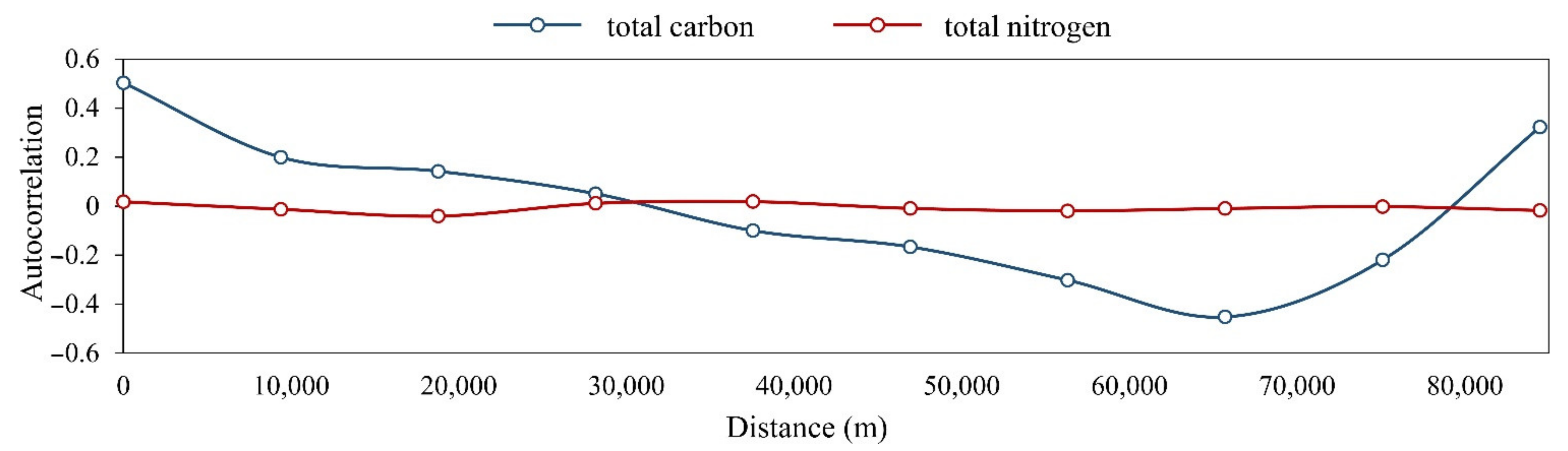
Table 3. Descriptive statistics of soil TC and TN from soil sampling data.
Soil PropertynMean
(mg 100 g–1)
CVShapiro–Wilk TestMoran’s I
W-Valuep-Value
TC1782.1610.6710.878<0.0010.536
TN1780.1640.5630.871<0.0010.041
TC: total soil carbon, TN: total soil nitrogen, CV: coefficient of variation.
Table 4. Prediction accuracy of soil TC and TN prediction using geostatistics and machine learning.
Soil PropertySpatial ResolutionValueOKRKRFEML
TC1000 mR20.5370.5270.7180.748
RMSE0.9840.9940.7680.521
NRMSE0.4550.4600.3550.241
250 mR20.5370.5270.7220.848
RMSE0.9840.9940.7630.319
NRMSE0.4550.4600.3530.148
30 mR20.5370.5270.719-
RMSE0.9840.9940.767-
NRMSE0.4550.4600.355-
TN1000 mR20.1890.1740.3310.498
RMSE0.0790.0800.0720.062
NRMSE0.4800.4860.4370.381
250 mR20.1890.1740.3270.626
RMSE0.0790.0800.0720.054
NRMSE0.4800.4860.4380.328
30 mR20.1890.1740.318-
RMSE0.0790.0800.072-
NRMSE0.4800.4860.441-
TC: total soil carbon, TN: total soil nitrogen, R2: coefficient of determination, RMSE: root-mean-square error, NRMSE: normalized root-mean-square error.
Table 5. Processing time required for soil TC and TN prediction using geostatistics and machine learning.
HardwareSoil PropertySpatial ResolutionProcessing Time (ms)
OKRKRFEML
WorkstationTC1000 m5329524198311,856
250 m10,9199213694740,276
30 m363,380368,729780,941-
TN1000 m49325120100011,897
250 m11,12110,992667240,574
30 m361,700364,715739,155-
LaptopTC1000 m6127569095711,441
250 m11,32210,607872040,085
30 m381,159379,951--
TN1000 m57155537105414,739
250 m11,430984210,60636,431
30 m378,083376,846--
TC: total soil carbon, TN: total soil nitrogen, OK: ordinary kriging, RK: regression kriging, RF: random forest, EML: ensemble machine learning.
Table 6. Pairwise comparison table for the weighting of cost–benefit components in AHP.
Criterion NameAccuracyTimeRobustnessScalabilityApplicabilityWeight
accuracy134680.493
time 12450.232
robustness 1340.153
scalability 130.079
applicability 10.042
n = 5, CI = 0.064, RI = 1.120, CR = 0.057.
Table 7. Calculation of cost–benefit scores for evaluated soil prediction methods.
MethodStandardized ValuesCost–Benefit Score
AccuracyTimeRobustnessScalabilityApplicability
OK0.0320.8980.2720.0001.0000.308
RK0.0000.9360.2430.0000.0000.255
RF0.4551.0000.0000.0260.5000.480
EML1.0000.0001.0001.0000.5000.747
OK: ordinary kriging, RK: regression kriging, RF: random forest, EML: ensemble machine learning.
Publisher’s Note: MDPI stays neutral with regard to jurisdictional claims in published maps and institutional affiliations.

