Growing Stock Volume Estimation for Daiyun Mountain Reserve Based on Multiple Linear Regression and Machine Learning

Abstract

Remote sensing provides an easy, inexpensive, and rapid method for detecting forest stocks. However, the saturation of data from different satellite sensors leads to low accuracy in estimations of the growing stock volume in natural forests with high densities. Thus, this study added actual data to improve the accuracy. The Daiyun Mountain Reserve was the study area. Landsat 8 operational land imager data were combined with remote sensing data and actual measurements. Multiple linear regression (MLR) and machine learning methods were used to construct a model for estimating the growing stock volume. The decision tree model showed the best fit. By adding the measured data to the model, the saturation could effectively be overcome to a certain extent, and the fitting effect of all the models can be improved. Among the estimation models using only remote sensing data, the normalized difference vegetation index showed the strongest correlation with the model, followed by the annual rainfall and slope. The decision tree model was inverted to produce a map of the accumulation distribution. From the map, the storage volume in the west was lower than that in the east and was primarily confined to the middle-altitude area, consistent with field survey results.

1. Introduction

The Daiyun Mountain Nature Reserve is a national nature reserve in China. It primarily comprises a natural Pinus taiwanensis forest and typical mountain forest ecosystem along the southeast coast [1,2]. The protected areas include specimen sites for insects and plants, wild orchids, biodiversity, and endangered plant and animal species [3,4]. Providing real-time monitoring of the vegetation accumulation in the reserve can provide theoretical and scientific support for the study of organisms in the reserve and for the preservation of its ecology. The growing stock volume (GSV) is a key indicator of the productivity in a country or region and varies regularly with the tree species and site conditions [5]. It is also a crucial and sensitive reference standard for assessing the dynamic changes in regional vegetation growth. The main foundation for creating forestry management plans and realizing the sustainable development of forest resources is a timely understanding of the current conditions and development trends of the GSV. The traditional techniques for monitoring GSV are based on first- and second-class forest resource surveys. These are disadvantageous due to the protracted inquiry cycle and high labor expenses involved. In recent decades, owing to transmissions from different sensors, the methods and technologies for extracting forest parameters using remote sensing technology have developed rapidly, allowing for multi-scale forest parameters to be obtained accurately and rapidly via remote sensing and showing the potential for dynamic monitoring and quantitative estimations of forest resources [6,7,8]. The current remote sensing data sources for estimations of GSVs are mainly optical and microwave remote sensing data [9,10,11]. Gao et al. [12] used thematic mapper remote sensing data and explored the correlations between several remote sensing factors and the GSV. They showed that the canopy density exerted the most significant effect on the GSV. Meng et al. [13] investigated the relationships between the GSV and each of the infrared and near-infrared bands and discovered strong correlations. Liao et al. [14] argued that textural features could significantly improve the estimation accuracy of the GSV, particularly for high-resolution images of complex forest structures. Obata et al. [15] conducted extensive research on estimating GSVs using Landsat series data. Their experimental results showed that the Landsat series’ remote sensing data are highly promising for estimating standard parameters.

In addition, scholars have addressed the saturation phenomenon in forest biomass estimation using remote sensing in recent years, but the studies are limited to extracting vegetation indexes [16,17]. However, the higher depression in forests is the main factor contributing to the saturation phenomenon in remote sensing estimations of the GSV [18]. Neither the normalized difference vegetation index (NDVI) nor the enhanced vegetation index (EVI) can overcome the saturation phenomenon in forest biomass estimations using remote sensing. Shen et al. [19] investigated the relationship between forest cover and the GSV and discovered that the above-ground GSV was not significantly correlated with the EVI and NDVI when the canopy cover exceeded the forest density. Therefore, in this study, environmental information and field survey data were introduced into a model to overcome the saturation phenomenon owing to the higher depressions in natural forests. The fitting accuracies of different models were derived, along with the degree of improvement from the field survey data for overcoming the saturation phenomenon on the fitting effect of the models.

Multiple linear regression (MLR) models primarily include two or more independent variables. They aim to use the best combinations of independent variables to predict dependent variables with high interpretability. Bolat et al. [20] used MLR models and concluded that the prediction accuracy for the GSV is closely associated with the forest’s vegetation structure and spatial dependence. Additionally, they mentioned that MLR models have difficulty in finding polynomial correlations between nonlinear data or data characteristics. Machine learning models can effectively solve this problem. Thus, three machine learning regression models were used in our study.

Recently, decision tree models have been increasingly used to analyze, describe, and predict ecological data, and the logic used in these modeling decision tree models can effectively handle various types of predictor variables (such as sparse, skewed, continuous, and categorical). The predictor and dependent variables do not require that any form of distributional assumptions can handle complex interactions among the predictor variables [21]. However, a single decision tree model has specific shortcomings, such as model instability (small changes in the data may cause large changes in the tree, thereby affecting the interpretation) and overfitting [12]. To overcome these problems, researchers have proposed integrated learning-based random forest models, in which many decision trees are combined to form a single model, and such integrated learning-based decision tree models are typically more stable and have better predictive power than single decision tree models [22]. Some scholars have used random forest models to analyze the sources of differences in estimating dependent variables according to various independent variables in ecology and forestry [23,24,25,26,27], which has solved the related scientific problems quite well. Extra Trees, compared with random forests, are extremely random in the division of decision tree nodes and directly use a random feature and a random threshold on the random feature for partitioning. Extra Trees provide a significantly strong additional randomness that does not bias the entire model by a few extreme sample points [28,29,30]. Therefore, in this study, three typical machine learning models were chosen for fitting: decision trees, random forests, and Extra Trees.

In recent years, many GSV estimation experiments have been conducted based on forest farms and plots; however, studies considering subcompartments and combinations of remote sensing images and field survey data in such subcompartments remain limited. Therefore, this study compared the performances of traditional regression and machine learning models in the Daiyun Mountain Reserve and the fitting accuracy changes before and after adding the field survey data of the subcompartments to the models.

2. Methods

The Daiyun Mountain Reserve is located in Dehua County, Fujian Province, China (118°05′22″ to 118°20′15″ E, 25°38′07″ to 25°43′40″ N). The location of the study site within Fujian Province as well as the location of Fujian Province with respect to China is shown in the Figure 1. The total reserve is 13,472.4 ha, and 5514.1 ha are occupied by the core area [31]. The highest elevation of the Daiyun Mountain Reserve is 1856 m, the lowest elevation is 650 m, and the relative elevation difference is 1206 m, resulting in significant vertical changes in climate and vegetation. The annual average temperature in the reserve is 15.6–19.5 °C, the annual average sunshine duration is 1875.4 h, and the annual average rainfall is 1700–2000 mm. The zonal vegetation type is the south subtropical monsoon evergreen broad-leaved forest. It comprises a narrow coniferous broad-leaved mixed forest belt at an altitude of 1000–1200 m, a Pinus taiwanensis coniferous forest at an altitude of 1200 m, and mountain shrubs at the top of the mountain, with a forest coverage rate of 93.4%.

2.1. Establishment of Daiyun Mountain Reserve Database

The GSV data used in this study were forest management inventory data of the Daiyun Mountain Reserve acquired by the Fujian Forestry Bureau in 2018. The GSVs of the broad-leaved forests and pine forests (moso bamboo was not counted) were calculated for each subcompartment in the Daiyun Mountain Reserve in the Figure 2.

In this study, SPTOOLS in the Arcgis 10.8 software (Environmental Systems Research Institute, Inc. RedLands, CA, USA) was used to obtain the weighted averages of the annual rainfall dataset with a resolution of 1 km in China (Chinese National Earth System Science Data Center) [32] and a digital elevation model dataset with a resolution of 90 m in the Fujian province in 2018 (Resource and Environment Science and Data Center) [33] on a small-class scale. An annual average rainfall, altitude, slope gradient, and slope direction were then assigned to each subcompartment.

2.2. Normalized Difference Vegetation Index (NDVI) Extraction and Data Preprocessing

The remote sensing images used in this study were captured from Landsat 8 operational land imager (OLI) data (Geospatial Data Cloud) [34] at path No. 119 and row No. 42 on 5 October 2018. ENVI5.3 software was used to preprocess the remote sensing data, including clipping, radiation calibration, and atmospheric correction. The NDVI was selected as the vegetation index, and its weighted average was assigned to each subcompartment. In this study, the NDVI was calculated as the sum of the values of the near-infrared (NIR) and visible red bands over the difference between the values of the NIR band (NIR < 0.7 mm) and visible red band (0.4 mm < R < 0.7 mm).

$$NDVI=\frac{NIR-R}{NIR+R}$$

(1)

In the above, NIR is the reflectance of the near-infrared band, and R is the reflectance of the visible red band.

In this study, the extracted environmental factors (Figure 3 and Figure 4) were normalized to ensure that each feature vector was treated equally by the classifier. The normalization formulas shown in

Table 1. Normalization formulas for eight environmental factors.

Data Type	Environmental Information	Normalization Formulas
Remote sensing data	NDVI	$x_1=\frac{B_{NIR}-B_R}{B_{NIR}+B_R}$	(2)
	Annual rainfall (mm)	$x_2=\frac{R-R_{\min }}{R_{\max }+R_{\min }}$	(3)
	Altitude (m)	$x_3=\frac{A-A_{\min }}{A_{\max }+A_{\min }}$	(4)
	Slope gradient (°)	$x_4=\sin x$	(5)
	Slope direction (°)	$x_5=\frac{\cos \beta +1}{2}$	(6)
Field measurement data	Tree height (m)	$x_6=\frac{H-H_{\min }}{H_{\max }+H_{\min }}$	(7)
	DBH (cm)	$x_7=\frac{D-D_{\min }}{D_{\max }+D_{\min }}$	(8)
	Tree age (year)	$x_8=\frac{N-N_{\min }}{N_{\max }+N_{\min }}$	(9)

were used to normalize the annual rainfall, altitude, slope gradient, slope direction, tree height, diameter at breast height (DBH), and tree age.

2.3. Selection of Regression Model

2.3.1. Multiple Linear Regression (MLR) (Model 1)

$$y={\beta }_0+{\beta }_1{x}_1+{\beta }_2{x}_2+\cdots +{\beta }_n{x}_n$$

(10)

In the above, y is the GSV per ha; β₀, β₁, ···, β_n is the model-fitting parameter; x₀, x₁, ···, x_n is the environmental information regarding the remote sensing and field measurement data; and n is the number of variables.

2.3.2. Decision Tree Regression (Model 2)

A continuous value prediction model using a tree structure divides the samples arriving at the node based on a specific attribute, and each subsequent branch of the node corresponds to a possible value of the attribute.

2.3.3. Random Forests (Model 3)

Many decision trees are generated in this process based on the modeling data set, sample observation, and characteristic variables. By performing random sampling, each time that the sampling results are based on a tree and a tree is generated based on its own attributes rules and values, the forest integrates all of the rules of the decision tree and the final judgment value.

2.3.4. Extra Trees (Model 4)

The “extra trees” algorithm is highly similar to the random forest algorithm. The random forest approach obtains the best bifurcation attribute in a random subset, whereas the extra trees approach obtains a bifurcation value randomly to bifurcate the decision tree.

2.3.5. Selection of Hyperparameters for Machine Learning Models

In the above machine learning model, the parameters (

Table 2. Hyperparameters of the three machine learning models.

Machine Learning Model	(a) *	(b)	(c)	(d)	(e)
Decision tree regression	2	1	10	50	-
Random forests	5	5	10	50	100
Extra trees	2	1	10	50	100

* (a): minimum number of samples for internal node splitting; (b): minimum number of samples for leaf nodes; (c): maximum depth of the tree; (d): the maximum number of leaf nodes; and (e): number of decision trees.

) to be set are: the (a) minimum number of samples for internal node splitting, (b) minimum number of samples for the leaf nodes, (c) maximum depth of the tree, and (d) maximum number of leaf nodes. If the sample size of an internal node is less than (a), no further splitting is performed. If the sample size of a leaf node is less than (b), it is pruned with its sibling nodes. The splitting stops when the depth of the tree reaches (c) to avoid infinite downward division. The number of leaf nodes stops splitting when it reaches (d) to avoid an infinite number of division categories. In addition, the random forest and limit tree models must also set the (e) number of decision trees. Increasing the number of decision trees improves the fitting ability, but it increases the computation time and overfitting probability. In addition, the sample size of the study data is large; thus, each decision tree is sampled with put-back.

2.4. Evaluation Indicator

In this study, the IBM SPSS Statistics 26 software was used to process the GSV per ha from the forest management inventory data from Daiyun Mountain Reserve in 2018. It was combined with remote sensing and field measurement data to fit Models 1 to 4. In the machine learning models (Models 2–4), to evaluate the estimation abilities of the different models, the data were randomly segregated into training data (70%) and verification data (30%), and the coefficient of determination (R²), root-mean-square error (RMSE), and relative root-mean-square error (rRMSE) were selected as evaluation indexes. The R², RMSE, and rRMSE were calculated as follows:

$$R^2=1-\frac{{\displaystyle {\sum }_{i=1}^n{(y_i-\widehat{y})}^2}}{{\displaystyle {\sum }_{i=1}^n{(y_i-\overline{y})}^2}}$$

(11)

$$RMSE=\sqrt{\frac{1}{n}{\displaystyle \sum _{i=1}^n{(y_i-\widehat{y})}^2}}$$

(12)

$$rRMSE=\frac{RMSE}{\overline{y}}\times 100\%$$

(13)

Here, y_i is the measured value of the GSV per ha of the subcompartment, $\widehat{y}$ is the estimated value of the GSV per ha of the subcompartment, $\overline{y}$ is the average measured value of the GSV per ha of the subcompartment, and n is the test sample size.

3. Results

3.1. Input of Environmental Data

The input data for the model are as follows: (1) average annual rainfall (mm): ranged from 201.10 to 1828.39 mm in 2018; (2) altitude (m): the highest peak elevation was 1776.23 m, and the lowest point elevation was 438.81 m; (3) slope gradient (°): ranged from 0° to 39.18°; (4) slope direction (°): ranged from 0° to 350.52°; (5) NDVI: the lowest NDVI in the study area was 0.227, and the highest was 0.887; (6) tree height (m): the highest tree height in the study area was 30.0 m; (7) DBH (cm): the largest DBH in the study area was 48.7 cm; and (8) tree age (year): the oldest tree in the study area was 91 years old.

3.2. Fitting Results and Accuracy Evaluation of Estimation Models

In all of the estimation models (Figure 5) used in this study, the inversion values for the lower levels (less than 100 m³·hm⁻²) were higher than the observed values, whereas the inversion values for the higher levels (exceeding 250 m³·hm⁻²) were lower than the observed values. This is a typical saturation phenomenon in the remote sensing estimations of the GSV.

As shown in

Table 3. Accuracy evaluation of various regression models (including multiple linear regression (MLR)) via the growing stock volume (GSV) estimation, including the root-mean-square error (RMSE) and relative root-mean-square error (rRMSE).

Regression Model	Only Remote Sensing Data			Inclusion of the Measured Data
	R2	RMSE	rRMSE	R2	RMSE	rRMSE
		(m3·hm−2)	(%)		(m3·hm−2)	(%)
Model 1 (MLR)	0.146	63.564	45.647	0.486	49.323	35.420
Model 2 (Decision tree)	0.427	50.377	33.081	0.696	36.685	24.090
	(0.511) *	(48.301)	(31.371)	(0.726)	(36.120)	(23.719)
Model 3 (Random forests)	0.234	57.882	38.010	0.482	49.578	32.557
	(0.398)	(54.289)	(35.650)	(0.783)	(32.180)	(21.132)
Model 4 (Extra trees)	0.371	52.784	34.662	0.644	39.730	26.090
	(0.388)	(54.025)	(35.477)	(0.687)	(38.654)	(25.383)

* The evaluation indexes of the training set data are in parentheses.

, compared with the conventional regression model, the machine learning model achieved a better fitting relationship. In the case involving only remote sensing data, the fitting effect of the conventional regression model was unsatisfactory, with an R² of only 0.146; in fact, the highest R² of the decision tree models among the machine learning models was only 0.427.

After adding the measured data, the saturation in the GSV was effectively overcome, and the fitting effect of all models was improved. The R² of all models improved by more than 0.2, the RMSE was reduced by more than 10 m³·hm⁻², and the rRMSE was reduced by more than 6%. The MLR model demonstrated the greatest effect, where after adding the measured data again, the R² increased by 0.34, the RMSE decreased by 14.241 m³·hm⁻², and the rRMSE decreased by 10.227%. Among all of the regression models, the decision tree regression model demonstrated the best fit. In the model using only remote sensing data, the test set R² was 0.427, the RMSE was 50.377 m³·hm⁻², and the rRMSE was 33.081%. By including the measured data, the test set R² of the decision tree model reached 0.696, with an RMSE of 36.685 m³·hm⁻² and an rRMSE of 24.090%. The test results from the decision tree model suggest that the estimation of the GSV is generalizable.

3.3. Evaluation and Comparison of Environmental Factors

The estimated values, standard errors, 95% confidence intervals of the fitted parameters, and variance inflation factor (VIF) from Model 1 (MLR) are listed in

Table 4. Fitting results of the MLR model (only remote sensing data).

Name	Parameter	Estimate	Standard Error	95% Confidence Intervals		VIF *
				Lower Limit	Superior Limit
	β0	−408.737	53.306	−513.336	−304.138
NDVI	β1	542.143	63.398	417.724	666.545	1.133
Annual rainfall	β2	52.555	17.603	18.014	87.097	1.300
Altitude	β3	4.663	11.338	−17.584	26.910	1.274
Slope gradient	β4	99.144	18.412	63.015	135.272	1.175
Slope direction	β5	39.572	7.057	25.725	53.419	1.032

* Variance inflation factor.

and

Table 5. Fitting results of the MLR model (including measured data).

Name	Parameter	Estimate	Standard Error	95% Confidence Intervals		VIF
				Lower Limit	Superior Limit
	β0	−276.255	42.222	−359.105	−193.405
NDVI	β1	299.159	50.833	199.412	398.906	1.192
Annual rainfall	β2	30.003	13.796	2.931	57.074	1.307
Altitude	β3	32.326	9.255	14.166	50.487	1.389
Slope gradient	β4	24.919	14.772	−4.067	53.905	1.238
Slope direction	β5	24.173	5.555	13.274	35.073	1.047
Tree height	β6	307.427	21.450	265.337	349.518	3.613
DBH *	β7	−111.418	17.811	−146.368	−76.468	3.437
Tree age	β8	138.416	12.683	113.528	163.304	1.554

* Diameter at breast height.

. Both the model using only the remote sensing data and the model using measured data in the MLR showed p-values of less than 0.001, indicating that the results were significant. The VIF values for the environmental factors of the models ranged from 1.103 to 3.316, i.e., less than 5, indicating that neither model was multi-collinear. The NDVI was the most highly correlated indicator with the MLR model using only remote sensing data. In the model, the altitude showed a low correlation with the other variables, and in the MLR model with measured data, the NDVI and tree height were the most highly correlated with the model among all of the parameters. The correlation between the tree height and the other measured parameters was stronger.

The neutral feature learning models for the machine are listed in

Table 6. Feature importance of all environmental parameters for different regression models.

Name	Feature Importance
	Only Remote Sensing Data				Inclusion of the Measured Data
	A 1	B 2	C 3	Average	A	B	C	Average
NDVI	45.3%	38.4%	37.4%	40.37%	8.9%	9.8%	8.2%	8.97%
Annual rainfall	17.4%	22.2%	13.1%	17.57%	6.0%	5.4%	4.0%	5.13%
Altitude	11.1%	11.7%	13.1%	11.97%	4.7%	5.8%	4.1%	4.87%
Slope gradient	18.6	19.4%	27.1%	21.70%	4.0%	5.5%	5.7%	5.07%
Slope direction	7.2	8.3%	9.3%	8.37%	1.0%	2.5%	2.3%	1.93%
Tree height	-	-	-	-	45.4%	42.8%	35.9%	41.37%
DBH	-	-	-	-	7.7%	5.3%	8.7%	7.23%
Tree age	-	-	-	-	22.4%	22.9%	31.2%	25.50%

¹ A: Decision tree; ² B: Random forests; ³ C: Extra trees.

. Among the machine learning models using only remote sensing data, the NDVI demonstrated the strongest correlation with the estimation models. Meanwhile, the least important feature of the model (the NDVI) showed a feature importance value of 37.4%, i.e., much higher than those of other environmental parameters. In addition to the NDVI, the annual rainfall and slope direction were strongly correlated with the estimation model, although the slope direction indicated a low feature importance value of only 8.37%. After including the measured data, the tree height and tree age became the dominant features in the machine learning models, with feature importance values of 45% and 22.4%, respectively. Compared with other measured data, the DBH showed a low feature importance value of 7.23%.

3.4. Inversion of Accumulation Based on Decision Tree Model

The decision tree model, which showed the best overall fit, was used to invert the GSV of the entire study area by using kriging interpolation to obtain a volume distribution of the Daiyun Mountain Reserve (Figure 6). The maximum and minimum estimated accumulations in the study area were 296.7 and 77.5 m³ hm⁻², respectively, i.e., within the range of 108.7–159.8 m³·hm⁻², and the accumulation was primarily distributed in the central part of the study area at a moderate altitude. The estimated accumulation was generally below 99.5 m³ hm⁻², consistent with the actual findings.

4. Discussion

In past studies, the climate, topography, human disturbance, and forest management activities have influenced changes in forest structure and accumulation to some extent. Zeng [35] developed a climate-sensitive individual tree biomass model by combining the mean annual temperature (T) and annual precipitation (P) to analyze the influence of climatic factors on biomass estimation, and the results showed that mean annual precipitation influences the predicted biomass. Propastin [36] used geographically weighted regression to conclude that a strong correlation exists between the vegetation and rainfall in central Sulawesi by modeling the relationship between the vegetation and climate. In addition, Propastin [37] included elevation effects in geographically weighted regression (GWR) when estimating the accuracy of above-ground biomass (ABG) models using spectral data from remote sensing. The results showed that geographically and altitudinal weighted regression (GAWR) significantly improved the prediction of ABG in the study area. Katherine [38] surveyed plant communities and measured key abiotic variables across forest–tundra ecotones in six alpine valleys. The results showed that plant communities vary more in slope direction and gradient than in elevation. Due to local laws, the Daiyun Mountain Reserve is not open to the public; thus, the influence of human factors and operations in this study area can be excluded. Therefore, this study chose to introduce the environmental information of rainfall, elevation, slope gradient, and slope direction to improve the accuracy of the estimated storage model.

Gherardo [39] compared the accuracy of k-nn algorithms with non-parameters in two study areas, the Mediterranean and Alpine ecosystems, using remotely sensed imagery combined with field measurements, testing 3500 different algorithm configurations and yielding rRMSEs between 22% and 28% and GSV estimates between 44% and 63% for the two study areas. No significant difference was observed between the rRMSE derived by Gherardo using a k-nn algorithm with parameters and the rRMSE from this study using the learning algorithm. Li [40] estimated the GSV of coniferous forests using multiple high-resolution remote sensing images and compared their model accuracy, and the results showed that the rRMSE based on four image datasets (GF-2, ZY-3, Sentinel-2, and Landsat 8) were 22.16%, 22.44%, 20.06%, and 24.73%, respectively. Li’s study obtained a model with high accuracy using only remote sensing imagery at high resolutions, but his experiments were conducted on planted conifer forests with weak saturation phenomena. In Hawrylo’s study [41], the prediction accuracy of the model created using only Sentinel-2A imagery was low, characterized by a high rRMSE of 35.14% and a low R² of 0.24. The fusion of IPC data with Sentinel-2 reflectance values provided the most accurate model: rRMSE = 16.95% and R² = 0.82. However, a significant accuracy was obtained using only the IPC-based model: rRMSE% = 17.26% and R²= 0.81. The results suggest that the IPC data from this experiment played a decisive role in estimating the model. This indirectly illustrates the value of including measured data in this study to improve the accuracy of the estimation model.

The study area was located in a subtropical monsoon zone, and the selected samples represented the dominant tree species in the study area. Therefore, the experimental results are beneficial for GSV estimation in the above-mentioned climatic zone; however, their applicability to other regions and other tree species requires further investigation.

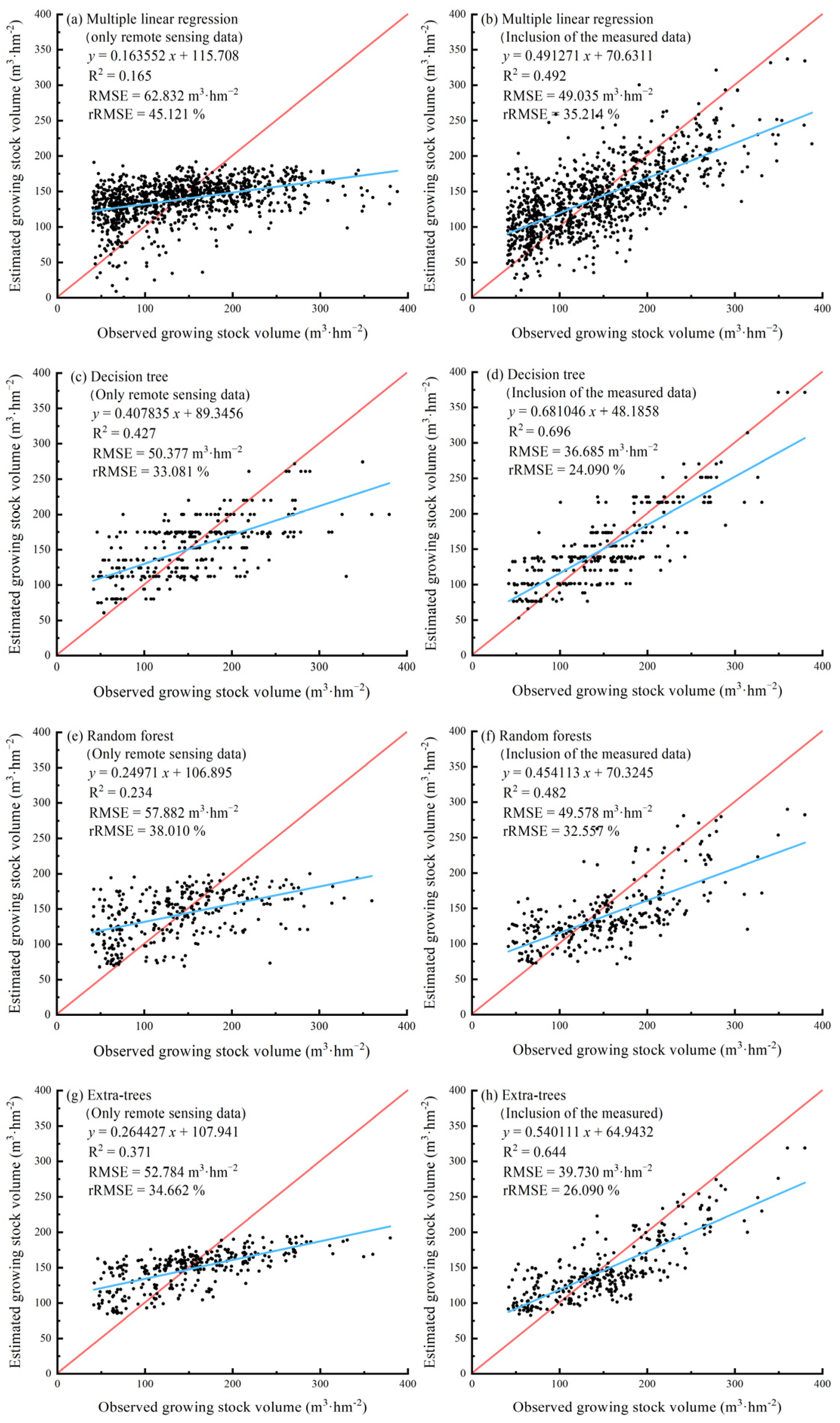
In this study, in addition to the environmental factors of the rainfall, topography, and elevation, the saturation of all estimation models was weakened after adding the measured data of the DBH and tree age to the models. Moreover, the difference between the inversion values of low and high levels and the observed values in the estimation model with measured data was significantly reduced; thus, the inclusion of the measured data can be considered to effectively alleviate the saturation caused by highly dense natural forests, to an extent. By comprehensively investigating the resource environment of the Daiyun Mountain Reserve, the GSV model can be even further improved by combining more environmental information, such as data regarding temperature, soil, natural disasters, and human interference.

This study selected the parameters of the machine learning models by manually adjusting the hyperparameters. The selection principle was that each parameter did not vary too much among the models while satisfying the good fitting effect of the models. Although this manual selection method does not guarantee the full performance of the model’s fitting ability [42], by manually adjusting the parameters between models several times, a trade-off can be obtained in determining the best combination of parameters and comparing the parameters with other models. This makes the models more comparable and generalizable [43,44].

In this study, Landsat 8 OLI data were used as the remote sensing data source; however, the information provided by the data was limited. Although various environmental information and field measurement data were used in this study, the saturation of the GSVs could not be entirely overcome. In future studies, we will investigate the use of synthetic aperture radar data-fusion methods to estimate the accumulation, which can subsequently be used to reduce the interference from saturation.

5. Conclusions

In this study, the Daiyun Mountain Reserve in Dehua County, Fujian Province, was selected as the study area, and small classes from the Forest Resources Type II survey were used as the units. The MLR and machine learning models were used to estimate the GSV in the study area by combining the Landsat 8 OLI data with badland data pertaining to the slope, slope orientation, elevation, and rainfall, and by adding measured data. The relevance of each variable in the estimation model was investigated. The main findings are as follows:

• The fitting results from the three machine learning regression models, i.e., the decision tree, random forest, and limit tree, were better than those of the classical MLR model. The decision tree model demonstrated the best fit with an R² of 0.696, RMSE of 36.685 m³ ∙ hm⁻², and rRMSE of 24.090%.
• To some extent, the inclusion of measured data in the model effectively mitigated the saturation caused by high-density natural forests, as well as effectively improving the fittings of both the MLR and machine learning models. The MLR model with and without measured data demonstrated the highest level of improvement; its R² value increased by 0.34, its RMSE decreased by 14.241 m³ ∙ hm⁻², and its rRMSE decreased by 10.227%.
• In the estimation model using only remotely sensed data, the NDVI showed the strongest correlation, followed by the annual rainfall and slope. The tree height and tree age were more relevant to the model than to the DBH after the small-group data were incorporated into the estimation model.
• The decision tree model was inverted to create a map of GSV distribution in the Daiyun Mountain Reserve. Based on the map, the storage volume in the west was lower than it was in the east, and the storage volume was primarily distributed in the middle elevation area from 945.84 to 1214.11 m, consistent with the results from the field survey.

References

1. Jiang, L.; He, Z.; Liu, J.; Xing, C.; Gu, X.; Wei, C.; Zhu, J.; Wang, X. Elevation Gradient Altered Soil C, N, and P Stoichiometry of Pinus taiwanensis Forest on Daiyun Mountain. Forests 2019, 10, 1089. [Google Scholar] [CrossRef]
2. Liu, J.; Su, S.; He, Z.; Jiang, L.; Gu, X.; Xu, D.; Ma, R.; Hong, W. Relationship between Pinus taiwanensis seedling regeneration and the spatial heterogeneity of soil nitrogen in Daiyun Mountain, southeast China. Ecol. Indic. 2020, 115, 106398. [Google Scholar] [CrossRef]
3. Ma, C.; Wu, L.; Zhao, L.; Zhang, Y.; Deng, Y.; Xu, Z. Holocene climate changes inferred from peat humification: A case study from the Daiyun Mountains, Southeast China. Quat. Int. 2021, 599–600, 15–23. [Google Scholar] [CrossRef]
4. Jiang, L.; He, Z.-S.; Gu, X.-G.; Liu, J.-F.; Feng, X.-P.; Zheng, S.-Q.; Xu, D.-W.; Liu, Y.-H. Classification and Ordination of the Pinus taiwanensis forest on Daiyun Mountain, Fujian Province, China. Taiwania 2020, 66, 119–128. [Google Scholar] [CrossRef]
5. Gschwantner, T.; Alberdi, I.; Bauwens, S.; Bender, S.; Borota, D.; Bosela, M.; Bouriaud, O.; Breidenbach, J.; Donis, J.; Fischer, C.; et al. Growing stock monitoring by European National Forest Inventories: Historical origins, current methods and harmonisation. For. Ecol. Manag. 2022, 505, 119868. [Google Scholar] [CrossRef]
6. Mura, M.; Bottalico, F.; Giannetti, F.; Bertani, R.; Giannini, R.; Mancini, M.; Orlandini, S.; Travaglini, D.; Chirici, G. Exploiting the capabilities of the Sentinel-2 multi spectral instrument for predicting growing stock volume in forest ecosystems. Int. J. Appl. Earth Obs. Geoinf. 2018, 66, 126–134. [Google Scholar] [CrossRef]
7. Puliti, S.; Saarela, S.; Gobakken, T.; Ståhl, G.; Næsset, E. Combining UAV and Sentinel-2 auxiliary data for forest growing stock volume estimation through hierarchical model-based inference. Remote Sens. Environ. 2018, 204, 485–497. [Google Scholar] [CrossRef]
8. Zhou, J.; Zhou, Z.; Zhao, Q.; Han, Z.; Wang, P.; Xu, J.; Dian, Y. Evaluation of Different Algorithms for Estimating the Growing Stock Volume of Pinus massoniana Plantations Using Spectral and Spatial Information from a SPOT6 Image. Forests 2020, 11, 540. [Google Scholar] [CrossRef]
9. López-Serrano, P.M.; Cárdenas Domínguez, J.L.; Corral-Rivas, J.J.; Jiménez, E.; López-Sánchez, C.A.; Vega-Nieva, D.J. Modeling of Aboveground Biomass with Landsat 8 OLI and Machine Learning in Temperate Forests. Forests 2019, 11, 11. [Google Scholar] [CrossRef]
10. Sterenczak, K.; Lisanczuk, M.; Parkitna, K.; Mitelsztedt, K.; Mroczek, P.; Misnicki, S. The influence of number and size of sample plots on modelling growing stock volume based on airborne laser scanning. Drewno 2018, 61, 201. [Google Scholar] [CrossRef]
11. Li, Y.; Li, M.; Li, C.; Liu, Z. Forest aboveground biomass estimation using Landsat 8 and Sentinel-1A data with machine learning algorithms. Sci. Rep. 2020, 10, 9952. [Google Scholar] [CrossRef] [PubMed]
12. Gao, Y.; Lu, D.; Li, G.; Wang, G.; Chen, Q.; Liu, L.; Li, D. Comparative Analysis of Modeling Algorithms for Forest Aboveground Biomass Estimation in a Subtropical Region. Remote Sens. 2018, 10, 627. [Google Scholar] [CrossRef]
13. Meng, Y.; Zhang, Y.; Li, C.; Zhao, J.; Wang, Z.; Wang, C.; Li, Y. Prediction of the Carbon Content of Six Tree Species from Visible-Near-Infrared Spectroscopy. Forests 2021, 12, 1233. [Google Scholar] [CrossRef]
14. Liao, Z.; He, B.; Quan, X. Potential of texture from SAR tomographic images for forest aboveground biomass estimation. Int. J. Appl. Earth Obs. Geoinf. 2020, 88, 102049. [Google Scholar] [CrossRef]
15. Obata, S.; Cieszewski, C.J.; Lowe, R.C.; Bettinger, P. Random Forest Regression Model for Estimation of the Growing Stock Volumes in Georgia, USA, Using Dense Landsat Time Series and FIA Dataset. Remote Sens. 2021, 13, 218. [Google Scholar] [CrossRef]
16. Kelsey, K.; Neff, J. Estimates of Aboveground Biomass from Texture Analysis of Landsat Imagery. Remote Sens. 2014, 6, 6407–6422. [Google Scholar] [CrossRef]
17. Dube, T.; Mutanga, O. Investigating the robustness of the new Landsat-8 Operational Land Imager derived texture metrics in estimating plantation forest aboveground biomass in resource constrained areas. ISPRS J. Photogramm. Remote Sens. 2015, 108, 12–32. [Google Scholar] [CrossRef]
18. Zhao, P.; Lu, D.; Wang, G.; Wu, C.; Huang, Y.; Yu, S. Examining Spectral Reflectance Saturation in Landsat Imagery and Corresponding Solutions to Improve Forest Aboveground Biomass Estimation. Remote Sens. 2016, 8, 469. [Google Scholar] [CrossRef]
19. Shen, M.; Chen, J.; Zhu, X.; Tang, Y.; Chen, X. Do flowers affect biomass estimate accuracy from NDVI and EVI? Int. J. Remote Sens. 2010, 31, 2139–2149. [Google Scholar] [CrossRef]
20. Bolat, F.; Bulut, S.; Günlü, A.; Ercanlı, İ.; Şenyurt, M. Regression kriging to improve basal area and growing stock volume estimation based on remotely sensed data, terrain indices and forest inventory of black pine forests. N. Z. J. For. Sci. 2020, 50. [Google Scholar] [CrossRef]
21. Ou, Q.X.; Li, H.K.; Lei, X.D.; Yang, Y. Difference analysis in estimating biomass conversion and expansion factors of masson pine in Fujian Province, China based on national forest inventory data: A comparison of three decision tree models of ensemble learning. Ying Yong Sheng Tai Xue Bao 2018, 29, 2007–2016. [Google Scholar] [CrossRef] [PubMed]
22. Zhu, Y.; Feng, Z.; Lu, J.; Liu, J. Estimation of Forest Biomass in Beijing (China) Using Multisource Remote Sensing and Forest Inventory Data. Forests 2020, 11, 163. [Google Scholar] [CrossRef]
23. Li, Y.; Li, C.; Li, M.; Liu, Z. Influence of Variable Selection and Forest Type on Forest Aboveground Biomass Estimation Using Machine Learning Algorithms. Forests 2019, 10, 1073. [Google Scholar] [CrossRef]
24. Pandit, S.; Tsuyuki, S.; Dube, T. Estimating Above-Ground Biomass in Sub-Tropical Buffer Zone Community Forests, Nepal, Using Sentinel 2 Data. Remote Sens. 2018, 10, 601. [Google Scholar] [CrossRef]
25. Ali, A.; Chen, H.Y.H.; You, W.-H.; Yan, E.-R. Multiple abiotic and biotic drivers of aboveground biomass shift with forest stratum. For. Ecol. Manag. 2019, 436, 1–10. [Google Scholar] [CrossRef]
26. Puliti, S.; Breidenbach, J.; Astrup, R. Estimation of Forest Growing Stock Volume with UAV Laser Scanning Data: Can It Be Done without Field Data? Remote Sens. 2020, 12, 1245. [Google Scholar] [CrossRef]
27. Chirici, G.; Giannetti, F.; McRoberts, R.E.; Travaglini, D.; Pecchi, M.; Maselli, F.; Chiesi, M.; Corona, P. Wall-to-wall spatial prediction of growing stock volume based on Italian National Forest Inventory plots and remotely sensed data. Int. J. Appl. Earth Obs. Geoinf. 2020, 84, 101959. [Google Scholar] [CrossRef]
28. Yu, R.; Yao, Y.; Wang, Q.; Wan, H.; Xie, Z.; Tang, W.; Zhang, Z.; Yang, J.; Shang, K.; Guo, X.; et al. Satellite-Derived Estimation of Grassland Aboveground Biomass in the Three-River Headwaters Region of China during 1982–2018. Remote Sens. 2021, 13, 2993. [Google Scholar] [CrossRef]
29. Tian, Y.; Huang, H.; Zhou, G.; Zhang, Q.; Tao, J.; Zhang, Y.; Lin, J. Aboveground mangrove biomass estimation in Beibu Gulf using machine learning and UAV remote sensing. Sci. Total Environ. 2021, 781, 146816. [Google Scholar] [CrossRef]
30. Arjasakusuma, S.; Swahyu Kusuma, S.; Phinn, S. Evaluating Variable Selection and Machine Learning Algorithms for Estimating Forest Heights by Combining Lidar and Hyperspectral Data. ISPRS Int. J. Geo-Inf. 2020, 9, 507. [Google Scholar] [CrossRef]
31. Ding, Q.; Lin, Z.; Liu, J.; Tu, W.; Huang, J.; Lan, S.; Hong, W. Optimum design of Daiyun Mountain nature reserve based on tail length. Sci. Silvae Sin. 2018, 54, 125–136. [Google Scholar]
32. National Earth System Science Data Center. Available online: http://www.geodata.cn/index.html (accessed on 11 December 2021).
33. Resource and Environment Science and Data Center. Available online: https://www.resdc.cn/data.aspx?DATAID=284 (accessed on 25 November 2021).
34. Geospatial Data Cloud. Available online: https://www.gscloud.cn/sources/index?pid=1&rootid=1 (accessed on 12 November 2021).
35. Zeng, W.; Chen, X.; Yang, X. Developing national and regional individual tree biomass models and analyzing impact of climatic factors on biomass estimation for poplar plantations in China. Trees 2020, 35, 93–102. [Google Scholar] [CrossRef]
36. Pavel Propastin, M.K.a.S.E. Application of Geographically Weighted Regression to Investigate the Impact of Scale on Prediction Uncertainty by Modelling Relationship between Vegetation and Climate. Int. J. Spat. Data Infrastruct. Res. 2008, 3, 73–94. [Google Scholar] [CrossRef]
37. Propastin, P. Modifying geographically weighted regression for estimating aboveground biomass in tropical rainforests by multispectral remote sensing data. Int. J. Appl. Earth Obs. Geoinf. 2012, 18, 82–90. [Google Scholar] [CrossRef]
38. Dearborn, K.D.; Danby, R.K. Aspect and slope influence plant community composition more than elevation across forest-tundra ecotones in subarctic Canada. J. Veg. Sci. 2017, 28, 595–604. [Google Scholar] [CrossRef]
39. Chirici, G.; Barbati, A.; Corona, P.; Marchetti, M.; Travaglini, D.; Maselli, F.; Bertini, R. Non-parametric and parametric methods using satellite images for estimating growing stock volume in alpine and Mediterranean forest ecosystems. Remote Sens. Environ. 2008, 112, 2686–2700. [Google Scholar] [CrossRef]
40. Li, X.; Long, J.; Zhang, M.; Liu, Z.; Lin, H. Coniferous Plantations Growing Stock Volume Estimation Using Advanced Remote Sensing Algorithms and Various Fused Data. Remote Sens. 2021, 13, 3468. [Google Scholar] [CrossRef]
41. Hawryło, P.; Wężyk, P. Predicting Growing Stock Volume of Scots Pine Stands Using Sentinel-2 Satellite Imagery and Airborne Image-Derived Point Clouds. Forests 2018, 9, 274. [Google Scholar] [CrossRef]
42. Weerts, H.J.P.; Mueller, A.C.; Vanschoren, J. Importance of Tuning Hyperparameters of Machine Learning Algorithms. arXiv 2020, arXiv:2007.07588. [Google Scholar]
43. McGibbon, R.T.; Hernández, C.X.; Harrigan, M.P.; Kearnes, S.; Sultan, M.M.; Jastrzebski, S.; Husic, B.E.; Pande, V.S. Osprey: Hyperparameter Optimization for Machine Learning. J. Open Source Softw. 2016, 1, 34. [Google Scholar] [CrossRef]
44. Probst, P.; Boulesteix, A.-L.; Bischl, B. Tunability: Importance of hyperparameters of machine learning algorithms. J. Mach. Learn. Res. 2019, 20, 1934–1965. [Google Scholar]
Figure 1. Location of Daiyun Mountain Reserve.
Sustainability 14 12187 g001
Figure 2. Growing stock volume (GSV) of each subcompartment in the Daiyun Mountain Reserve in 2018.
Sustainability 14 12187 g002
Figure 3. Remote sensing data (ae) of each subcompartment in the Daiyun Mountain Reserve in 2018.
Sustainability 14 12187 g003
Figure 4. Field measurement data (ac) of each subcompartment in the Daiyun Mountain Reserve in 2018.
Sustainability 14 12187 g004
Figure 5. Scatter plots of estimated vs. observed GSV (ah).
Sustainability 14 12187 g005
Figure 6. Spatial distribution of GSV as estimated by the decision tree model.
Sustainability 14 12187 g006