Brittleness Evolution Model of the Supply Chain Network Based on Adaptive Agent Graph Theory under the COVID-19 Pandemic

Abstract

The triggering of supply chain brittleness has a significant impact on enterprise benefits under attack from the COVID-19 pandemic. The complexity of the supply chain system, the uncertainty of the COVID-19 pandemic, and demand uncertainty have made the triggering and propagation of supply chain brittleness complicated. In this study, a brittleness evolution model based on adaptive agent graph theory has been constructed. The parameters of brittleness evolution, including brittleness entropy and the vertex state value, have been quantitatively designed, and the brittleness evolution model in which the adaptability of nodes is considered and is not considered is constructed. A simulation algorithm based on the integrated scheduling model of the supply chain has been established. Finally, the practicability of the proposed model and algorithm is demonstrated via a case study of an electronic supply chain network. The results indicate that the proposed model and algorithm can effectively analyze the brittleness evolution law of the supply chain under the impact of the COVID-19 pandemic, including the evolution law of the vertex state, the brittleness entropy of the vertex, the global entropy of brittleness, the seasonal evolution law of the supply chain brittleness, and the evolution law of the brittleness behavior.

1. Introduction

In the context of the economic globalization, the outbreak of the COVID-19 pandemic has had a huge impact on the security of the global supply chain system, which is a complex giant system with dissipative structure. The development of modern science and technology and the social division of labor make the supply chain networked and complicated, the trend of which is increasingly obvious. And the characteristic of the complex network is gradually shown in the supply chain system [1], which has made it extremely unstable in the process of operation and development. When attacked by uncertain events such as the COVID-19 pandemic, the security and reliability of the supply chain system are directly threatened [2,3].

Under the trend of globalization, business models such as production outsourcing and lean manufacturing have been adopted, which reduce costs and improve efficiency, while making the supply chain system more vulnerable [4]. The collapse of any node may trigger the brittleness of the whole system and lead to the collapse of the entire supply chain network, which would bring huge economic losses to enterprises [5]. Therefore, grasping the brittleness evolution law of the supply chain system to reduce and eliminate the impact of the COVID-19 pandemic has become an important issue in the field of supply chain security [6,7].

In this paper, the evolution model and simulation algorithm of supply chain brittleness are discussed. The research objectives are as follows:

• The evolution law of the vertex state of the uncertain supply chain under COVID-19 attack will be analyzed.
• The evolution law of brittleness entropy of the vertex in the supply chain will be solved.
• The evolution law of the global brittleness entropy of the uncertain supply chain will be demonstrated.
• The seasonal evolution law of the uncertain supply chain brittleness will be illustrated.
• The evolution law of the brittleness behavior of the uncertain supply chain will be solved.

The innovations and contributions of this paper are as follows:

• The model and algorithm of the vertex state and brittleness entropy of the vertex of the uncertain supply chain are established.
• The brittleness evolution model of the supply chain based on the adaptive agent graph is constructed.
• The simulation algorithm of the brittleness evolution of the uncertain supply chain based on the adaptive agent graph is designed.

The rest of the paper is organized as follows: The second section is a literature review; the third section describes the study and defines the problem; in Section 4, the model of brittleness evolution of the supply chain based on the adaptive agent graph is established. In Section 5, a simulation algorithm of the brittleness evolution of the supply chain is designed. In the sixth section, an example is simulated, and the results are analyzed. The seventh part concludes the whole paper.

2. Literature Review

2.1. Supply Chain Vulnerability

The academic world has paid great attention to the study of supply chain vulnerability. The existing research mainly focuses on the aspects of the identification of supply chain vulnerability factors, the evaluation of supply chain vulnerability, and the mechanism of correlation and influence of the supply chain vulnerability.

• The identification of vulnerability factors of the supply chain

For the study on the identification of vulnerability factors, Nakatani et al. [8] developed a model of supply chain structure with a graph and adjacency matrix based on graph theory, in which the vulnerability factors of the supply chain of Japanese synthetic resin were identified and measured. Sharma et al. [9] adopted the method of a fuzzy decision-making trial and evaluation laboratory (DEMATEL) to analyze the causal relationship of vulnerability factors of the supply chain of manufacturing, in which the vulnerability factors were identified. Based on the method of the Petri net and triangularization clustering algorithm, Blackhurst et al. [10] identified the vulnerable points of the supply chain network.

2.

Evaluation of supply chain vulnerability

The study of supply chain vulnerability evaluation mainly focuses on two aspects, including quantificational research of vulnerability value and the evaluation of vulnerability factors. In the quantitative study of vulnerability value, Wagner et al. [11] quantified the vulnerability value of the supply chain based on the method of graph theory, in which the effectiveness of different mitigation strategies of vulnerability was compared. Karwasra et al. [12] adopted the method which combined the interpretive structural modeling (ISM) and graph theory to construct a model to calculate the index of supply chain vulnerability.

As for the research of evaluation analysis of vulnerability factors of the supply chain, the existing studies mainly adopted the means of questionnaire surveys and interviews with industry experts to evaluate the vulnerability based on the fuzzy theory and gray theory. Ekanayake et al. [13] evaluated and analyzed the vulnerability factors of the supply chain of industrial construction in Hong Kong via the significance analysis of questionnaire data. Sharma et al. [14] used the method of an analytic hierarchy process (AHP) to evaluate the relative criticality of vulnerability factors of the supply chain of manufacturing. Majumdar et al. [15] developed a vulnerability factor matrix of the supply chain with the method of a fuzzy analytic hierarchy process (FAHP) and evaluated and analyzed the vulnerability factors of the supply chain of green apparel in South and Southeast Asia. Liu et al. [16] calculated the correlation degree of vulnerability factors of the supply chain based on the supply chain operation reference (SCOR) model and adopted the Kendall’s Tau coefficient to measure the effect of different assessment methods of supply chain vulnerability.

3.

Mechanism of correlation influence of supply chain vulnerability

The existing studies on the mechanism of correlation influence of supply chain vulnerability mainly focus on the influence of external factors on supply chain vulnerability, the relationship between supply chain structure and vulnerability, and the correlation between the vulnerability and other attributes of the supply chain.

The analysis of influence of external factors on supply chain vulnerability mainly included the following contents. Naghshineh et al. [17] studied the influence of additive manufacturing technology adoption on supply chain vulnerability. Ruel et al. [18] qualitatively analyzed that knowledge management could reduce the vulnerability of the supply chain. Bassett et al. [19] analyzed the vulnerability of the supply chain of the small-scale fishery supply chain (SSF) under the attack of the COVID-19 pandemic. Viljoen et al. [20] quantificationally studied the impact of the infrastructure of urban roads on supply chain vulnerability from the perspective of redundancy and overlap of shortest paths. Saengchai, S. and Jermsittiparsert, K. [21] adopted the survey-based methodology and used the SEM-PLS technique to test the hypothesized relationships to analyze the influencing factors of lean production practice, which provided a helpful perspective to understand the issue of supply chain vulnerability.

As for research on the relationship between the structure and vulnerability of the supply chain, Ma et al. [22] analyzed the influence of the supply chain’s structure on vulnerability from the angle of three indexes including the clustering coefficient, maximum connectivity, and network connectivity. Wagner et al. [23] empirically studied the relationship between firm performance and vulnerability, between structure category and vulnerability, and between management category and vulnerability based on the graph theory. Shughrue et al. [24] quantificationally analyzed the relationship between the structural elements of the global industrial supply chain network such as the node strength, the node association strength, and vulnerability from the perspective of the network scale.

The previous studies, respectively, analyzed the relationship between supply chain vulnerability and other attributes from different perspectives [25,26,27]. Kurniawan et al. [25] studied the impact of mitigation strategies of vulnerability on the supply chain’s effectiveness, which took risk culture as a moderating factor. Bai et al. [26] adopted the method which combined case study and consensus qualitative research (CQR) to empirically analyze the development law of vulnerability and the resilience of the tourism supply chain under the attack of the COVID-19 pandemic. Zhang et al. [27] constructed a model of the balance state of supply chain vulnerability and elasticity with the method of the integrating fuzzy analytic hierarchy process (AHP) and the fuzzy technique for order of preference by similarity to an ideal solution (TOPSIS).

4.

Conceptual differences between supply chain vulnerability and supply chain brittleness

The studies above aimed to evaluate and analyze the vulnerability factors and their impacts on the supply chain. However, supply chain vulnerability would lead to the collapse of the whole system, which is a cross topic between the area of supply chain security and complex systems. The existing studies have not quantificationally analyzed the mechanism of supply chain disruption and collapse caused by vulnerability from the perspective of complex systems engineering theory.

In view of this, we proposed a concept of supply chain brittleness in this paper, which leans towards the concept of physics, to distinguish from the previous research of “supply chain vulnerability” and define the focus of this paper, which is that the internal mechanism of the supply chain’s collapse caused by the failure of a single node would be quantificationally analyzed.

2.2. Brittleness Theory of Complex Systems

The concept of the brittleness of complex systems was proposed by Enjie Luan, the former deputy director of the Commission of Science, Technology and Industry for National Defense of the PRC in 2001, and the origin of the theory is that local factors would cause the global collapse. Subsequently, the team of Professor Hongzhang Jin systematically conducted the research on the brittleness of complex systems from the perspectives of the catastrophe theory, brittleness entropy, the theory of self-organized criticality, and the graph theory [27].

• Brittleness of complex systems based on catastrophe theory

Existing studies have studied the brittleness of complex systems based on the catastrophe theory [28,29,30,31,32,33,34]. Guo et al. [28,30,31,33] proposed a method of establishing the model of potential function of brittleness from the perspective of catastrophe theory. Wu et al. [29] conducted a quantitative analysis of the brittleness of traffic systems and found that the control strategies of traffic systems are more effective when the observed density of traffic flow is close to the critical density. Li et al. [32,34] analyzed the brittleness of SARS with the method of a mutational potential function.

2.

Brittleness entropy of complex systems

For the study of brittleness entropy of complex systems, Wei et al. [35] defined the concepts of brittleness entropy and the fundamental elements of brittleness based on the theory of set pair analysis. Cao et al. [36] proposed a non-cooperative game model based on the concept of brittleness entropy to predict the cascade failure of the subsystems in a complex system. Wei et al. [37,38] quantificationally analyzed the propagation mechanism of brittleness of SARS based on the brittleness entropy theory.

3.

Brittleness of complex systems based on the theory of self-organized criticality

Some scholars have studied the brittleness of complex systems from the perspective of the theory of self-organized criticality. Yan et al. [39,40] systematically analyzed the brittleness of the power network, established a two-dimensional brittleness model of power systems based on the sandpile model of the theory of self-organized criticality, and analyzed the conditions of brittleness triggering via simulation experiments.

4.

Brittleness of complex systems based on graph theory

It is also an important research direction to study the brittleness of complex systems based on the graph theory [41,42,43]. Wu et al. [41] established the relationship graph of the brittleness between subsystems of a complex system and calculated the brittleness degree of the brittleness source based on the probability of the brittleness propagation and the collapse probability of the brittleness source. Wang et al. [42] analyzed the brittleness of the highway network of transportation systems and put forward a calculation method of the index of the brittleness source. Lin et al. [43] proposed the concept of an agent graph, in which the graph of the transportation system, which was weighted and directed, was constructed, and the rules of collapse evolution of the subject were analyzed.

2.3. Research Summary

The brittleness theory of complex systems has not been applied to the problem of supply chain collapse in the studies above. As for supply chain brittleness, Yan et al. [44] only qualitatively analyzed the brittleness of the supply chain from conceptual perspectives, such as brittleness entropy, co-brittleness entropy, and brittleness relationship entropy. And the problem of the evolution mechanism of supply chain brittleness has not been quantificationally analyzed.

Therefore, we introduce the concept of brittleness entropy in this study to quantificationally compute the brittleness value of the supply chain, and the algorithm has also been designed. Based on the adaptive agent graph theory and the information entropy theory, the brittleness evolution model of the supply chain was constructed to quantificationally analyze the rules of the brittleness evolution of the supply chain. And on the basis of our published research [45], the integrated scheduling model of the uncertain supply chain was adopted as the auxiliary technology element, and a simulation algorithm of the brittleness evolution of the supply chain was designed.

3. Study Description and Problem Definition

3.1. Study Description

Under the impact of the COVID-19 pandemic, the mechanism of supply chain disruption and collapse is that the supply chain complex system has the attribute of brittleness. When a node in a supply chain collapses, due to the existence of brittleness relations between nodes, the node which has the relationship with the brittleness node may also collapse. When most of the nodes in the system have failed, the supply chain can be disrupted or even collapse.

Based on the adaptive agent graph theory, the evolution model and simulation algorithm of supply chain brittleness will be constructed in this paper. And we mainly study the following problems: The evolution law of the vertex state of the uncertain supply chain, the evolution law of brittleness entropy of supply chain nodes, the evolution law of global brittleness entropy, the seasonal evolution law of supply chain brittleness, and the evolution law of the brittleness behavior of the supply chain.

3.2. The Adaptive Agent Graph of the Supply Chain Brittleness Network

Based on the adaptive theory [43], in this study, the adaptive agent graph of the supply chain brittleness network is defined as follows:

• Vertexes: the suppliers, manufacturers, distributors, and end retailers of the supply chain are defined as the vertexes of the adaptive agent graph of the brittleness network.
• Arcs: The directed link a which connects the ordered vertex pairs i and j is defined as the arc of the adaptive agent graph of the supply chain brittleness network, denoted as a = <i, j>. Link a has both the meaning of directionality (vertex i and vertex j, respectively, represent the starting point and the ending point) and weight value.
• Adjacency relation: Whether there is a brittleness link between vertex i and vertex j is defined as the adjacency relation of the adaptive agent graph in this paper. If there is a brittleness link, r_ij = 1, r_ij ∈ R; otherwise, r_ij = 0. The mathematical expression is as follows:

  $$r_{ij}=\{\begin{array}{cc}1& <i,j>\in A\\ 0& <i,j>\notin A\end{array}$$

  (1)
• Topological structure: The weighted and directed graph D = <V,A,R> is defined as the topological structure of the adaptive agent graph, which is the graphic representation of the brittleness relationship of supply chain complex systems.
  Thereinto, V(i, j ∈ V) represents the vertex set of a supply chain brittleness network. A(a ∈ A) represents the directed link set of a brittleness network, and R(r_ij∈ R) represents the set of adjacency relations between vertex i and vertex j.
• The Flow of vertex: The entropy flow of supply chain nodes is defined as the flow of a vertex of an adaptive agent graph of a supply chain brittleness network. And the adjacency relationship would be obtained through the distribution results of the flow of vertex.
• The weight of adaptive agent graph: The proportion of the quantity of material flow supplied from vertex i to vertex j to total material flow of vertex i is defined as the weight ω_ij of the adaptive agent graph of the supply chain brittleness network.
• The interaction between vertexes: the transferring and exchanging of entropy flow between vertexes are defined as the interaction between vertexes in the adaptive agent graph of the supply chain brittleness network.
• The memory function of the vertex: the memory function is composed of the vertex state function and the entropy flow function of the vertex, which is used to store the state, the entropy flow, and brittleness evolution rules of each vertex.
• The global energy function: The global energy function reflects the disorder degree of the supply chain brittleness network and also reflects the superposition effect of the brittleness behavior of vertexes. In this study, the weighted sum of all brittleness entropy (the global brittleness entropy) of the supply chain brittleness network is defined as the global energy function of the adaptive agent graph.

3.3. The Problem Definition of Brittleness Evolution of the Supply Chain

According to the stimulus–response model of the individual adaptive behavior in complex systems established by Holland [46], the updating process of an adaptive vertex consists of four parts, including perception, storage, control, and response. Based on the improvement of control systems in the model by Lin et al. [43], in this study the problem of the brittleness evolution of the supply chain is described as follows:

Taking vertex i as an example, the flow f_i(k) for i is updated by the dynamic model and becomes f_i(k + 1) in times of k + 1, and the mapping, φ is the program execution function. According to the dynamic evolution model of the adaptive agent graph [43], f_i(k + 1) is described as follows:

f_i(k + 1) = φ f_i(k), r)

(2)

Thereinto, r is the external disturbance condition of the supply chain. That is to say, the value of the flow of vertex i in times of k + 1 is jointly determined by the flow of vertex i in times of k and the external disturbance.

f_i(k + 1) is the input of the actuator in times of k + 1, denoted as $f_i^{input}\left(k+1\right)$. As an adaptive agent, S^j (j = 1, …, l) is defined as the decision condition, and the relationship between the state value x_i(k + 1) and the flow value f_i(k + 1) is determined by the rules in the actuator of “IF/THEN” as follows:

$$\mathrm{IF} f_i^{input}\left(k+1\right)\in S^1, \mathrm{THEN} x_i\left(k+1\right)={\phi }_i^1\left(f_i^{input}\left(k+1\right),\mathrm{r}\right)$$

(3)

$$\mathrm{IF} f_i^{input}\left(k+1\right)\in S^l, \mathrm{THEN} x_i\left(k+1\right)={\phi }_i^l\left(f_i^{input}\left(k+1\right),\mathrm{r}\right)$$

(4)

The controller entrusts the vertex agent of the supply chain with the adaptability and purpose. The state value of the vertex in times of k + 1 can be obtained after the vertex flow passes through the controller as follows:

$$x\left(k+1\right)=\left(x_1\left(k+1\right), x_2\left(k+1\right), x_3\left(k+1\right), \dots x_n\left(k+1\right)\right)$$

(5)

And the vertex state determines the value of flow as follows:

$$f_i\left(k+1\right)=F\left(x_i\left(k+1\right)\right)$$

(6)

4. Problem Formulation

4.1. The Brittleness Evolution Model of Adaptive Agent Graph of the Supply Chain

• Assumptions
  According to Holland’s CAS (complex adaptive systems) theory [46], the evolutionary steps of vertexes of the adaptive agent graph of the supply chain are set as follows:

  (1)

  Each vertex senses the entropy flow from other agents and the increase of entropy caused by external environmental interference through the detector. And then, the entropy flow of the vertex is determined according to its own state value.

  (2)

  The memory function of the vertex is established to store its own state, the entropy flow, and other information into the memory, and the knowledge base is preliminarily constructed.

  (3)

  The vertex constantly learns from the knowledge base and establishes the control strategies. A series of IF/THEN rules are established to continuously learn memory functions, and the vertex state and vertex entropy flow are updated to update the knowledge base in the memory.

  (4)

  According to the interaction process of entropy flow, the vertex entropy flow is output through the reactor, and the vertex state is output through the flow function φ. The relationship between the vertex state value $x_i^{t+1}$ and the entropy flow value $f_i^{t+1}$ is determined by the IF/THEN rules in the actuator.

  (5)

  The updated flow $f_i^{t+1}$ of the vertex agent would be used as input to the actuator in times of t + 1.

• The brittleness evolution model of the vertex of the adaptive agent graph of the supply chain

(1)

When the adaptive behavior of the vertex is not considered, the entropy flow evolution model of the vertex is

$$f_i^{input}\left(t+1\right)=f_i\left(t\right)-{\displaystyle \sum }_j{\omega }_{ij}{f}_i\left(t\right)+{\displaystyle \sum }_s{\omega }_{si}{f}_s\left(t\right)+r_i\left(t\right)$$

(7)

Thereinto, r_i(t) is the random disturbance of the external environment to the vertex i.

The IF/THEN rules are established as follows:

IF $0<f_i^{input}\left(t+1\right)<logA$, THEN $x_i\left(t+1\right)={\phi }_i\left(f_i^{input}\left(t+1\right)\right)$;

IF $f_i^{input}\left(t+1\right)\le 0$, THEN $x_i\left(t+1\right)=1;$

IF $f_i^{input}\left(t+1\right)\ge logA$, THEN $x_i\left(t+1\right)=1.$

Thereinto, the mapping ${\phi }_i^l\left(j=1,\dots ,l\right)$ is the executive function that determines the vertex state.

The equation of the vertex state is

$$x_i\left(t+1\right)=\{\begin{array}{cc}{e}^{-f_i^{input}\left(t+1\right)}& 0\le f_i^{input}\left(t+1\right)\le logA\\ 1& f_i^{input}\left(t+1\right)\le 0\\ 1& f_i^{input}\left(t+1\right)\ge logA\end{array}$$

(8)

According to Equations (6)–(11), the equation of the entropy flow of the vertex is

$$f_i\left(t+1\right)=\{\begin{array}{cc}{f}_i^{input}\left(t+1\right)& 0\le f_i^{input}\left(t+1\right)\le logA\\ 0& f_i^{input}\left(t+1\right)\le 0\\ 0& f_i^{input}\left(t+1\right)\ge logA\end{array}$$

(9)

(2)

When the adaptive behavior of the vertex is considered, the brittleness connection between vertexes is built through the distribution of entropy flow, and the evolution model of entropy flow of the vertex is

$$f_i^{input}\left(t+1\right)=f_i\left(t\right)-{\displaystyle \sum }_j{\omega }_{ij}{f}_i\left(t\right)+{\displaystyle \sum }_s{\omega }_{si}{f}_s\left(t\right)+r_i\left(t\right)$$

(10)

The IF/THEN rules are established as follows:

IF $f_i^{input}\left(t+1\right)\in S$, THEN $x_i\left(t+1\right)={\phi }_i\left(f_i^{input}\left(t+1\right)\right)$

IF $f_i^{input}\left(t+1\right)\le 0$, THEN $x_i\left(t+1\right)=1$

IF $f_i^{input}\left(t+1\right)\ge logA$, THEN $x_i\left(t+1\right)=I_i\left(t-1\right)/I_i\left(t\right)$

The equation of the vertex state is

$$x_i\left(t+1\right)=\{\begin{array}{cc}{e}^{-f_i^{input}\left(t+1\right)}& 0\le f_i^{input}\left(t+1\right)\le logA\\ 1& f_i^{input}\left(t+1\right)\le 0\\ I_i\left(t-1\right)/I_i\left(t\right)& f_i^{input}\left(t+1\right)\ge logA\end{array}$$

(11)

According to Equation (21), the equation of the entropy flow of the vertex is

$$f_i\left(t+1\right)=\{\begin{array}{cc}{f}_i^{input}\left(t+1\right)& 0\le f_i^{input}\left(t+1\right)\le logA\\ 0& f_i^{input}\left(t+1\right)\le 0\\ I_i\left(t-1\right)/I_i\left(t\right)& f_i^{input}\left(t+1\right)\ge logA\end{array}$$

(12)

Thereinto, I_i(t) is the memory function of the supply chain system, and the memory function of the vertex state is as follows:

$$I_i\left(t+1\right)=I_i\left(t-1\right)+x_i\left(t\right)$$

(13)

The memory function of the entropy flow of the vertex is as follows:

$$I_i\left(t+1\right)=I_i\left(t-1\right)+f_i\left(t\right)$$

(14)

4.2. Model of Maximum/Minimum Brittleness Collapse Path of the Supply Chain

Suppose there are m pairs of OD, there are n collapse paths h_i(i = 1, 2, …, n) from manufacturers to retailers, and the maximum and minimum crash paths need to satisfy the following formula [47]:

$$Z=ma{x}_{H\in E\left(h_i\right)}\left({\displaystyle \prod }_{a\in h_i}\omega \left(a\right)\right)\mathrm{or} {min}_{H\in E\left(h_i\right)}\left({\displaystyle \prod }_{a\in h_i}\omega \left(a\right)\right),\left(i=1,2,\dots ,n\right)$$

(15)

Thereinto, ω(a) represents the weight value of link a on the crash path h_i.

The constraint is as follows:

$$s.t.{\displaystyle \sum }_{j:ij\in E}{\theta }_{ij}-{\displaystyle \sum }_{j:ji\in E}{\theta }_{ji}=\{\begin{array}{cc}1& i=o\\ 0& i\in N-\left\{o,d\right\}\\ -1& i=d\end{array}$$

(16)

Thereinto, θ_ij a is a binary variable: if the link a ∈ <i,j,> is contained by the crash path h_i, the value is 1; otherwise, it is 0.

And the weight of the supply chain link a which contains vertex i is

$$\omega \left(a\right)={\omega }_{ij}={\omega }_{mspqt}=\frac{Q_{mspqt}^{SD}}{Q_{mspt}^{SD}}$$

(17)

ω_mspqt is the weight value of link pq under the demand scenario m and the brittleness scenario s in period t, $Q_{mspqt}^{SD}$ is the flow value of link pq under the demand scenario m and the brittleness scenario s in period t, and $Q_{mspt}^{SD}$ is the flow value of the node p of a supply chain network under the demand scenario m and brittleness scenario s in period t.

The weight of the collapse path h_i which contains vertex i is

$$\begin{gathered} {\omega }_{h_i}=P\left(B_{i_n}{B}_{i_{n-1}}\dots B_{i_1}|B_{i_1}\right)=\frac{P\left(B_{i_n}{B}_{i_{n-1}}\dots B_{i_1}\right)}{P\left(B_{i_1}\right)} \\ = \frac{P\left(B_{i_2}{B}_{i_1}\right)}{P\left(B_{i_1}\right)}\frac{P\left(B_{i_3}{B}_{i_2}{B}_{i_1}\right)}{P\left(B_{i_2}{B}_{i_1}\right)}\dots \frac{P\left(B_{i_n}{B}_{i_{n-1}}\dots B_{i_1}\right)}{P\left(B_{i_{n-1}}\dots B_{i_1}\right)} \\ = P\left(B_{i_2}|B_{i_1}\right) P\left(B_{i_3}|B_{i_2}{B}_{i_1}\right)\dots P\left(B_{i_n}|B_{i_{n-1}}\dots B_{i_1}\right) \\ = {\omega }_{i_1{i}_2}{\omega }_{i_2{i}_3}\dots {\omega }_{i_{n-1}{i}_n} \end{gathered}$$

(18)

4.3. Calculation Model of Brittleness Evolution Parameters

• The collapse probability of vertex i under normal scenarios is

  $$P_i=\frac{C\left(i\right)}{C_k\left(i\right)}$$

  (19)

Thereinto, C(i) represents the load of the vertex i of the supply chain, and C_k(i) is the capability value of the vertex i.

2.

The probability of the brittleness event s of a supply chain is

$$\begin{gathered} P_s={\displaystyle \prod }_{i\in I_s}\left(1-p_i\right){\displaystyle \prod }_{i\in I|I_s}{p}_i \\ i\in I_s, \forall m,s \end{gathered}$$

(20)

And the load of the vertex i is

$$C\left(i\right)={\displaystyle \sum }_{o\ne d\ne i}\frac{{\delta }_{od}\left(i\right)}{{\delta }_{od}}$$

(21)

Thereinto, ${\delta }_{od}\left(i\right)$ is the number of shortest paths through vertex i between vertex O, and δ_od is the number of shortest paths between vertex O and D.

The capability value of the vertex i is

$$C_k\left(i\right)=C_0\left(i\right)\left(1+\alpha \right)$$

(22)

C₀(i) is the initial load of the vertex i of the supply chain, and α is the tolerance coefficient.

The degree of the vertex i is

$$d_i={\displaystyle \sum }_{l\in E}{\delta }_l\left(i\right)$$

(23)

3.

The scheduling model of the brittleness network of the supply chain is [44]

$$F=min[\gamma f_1+\left(1-\gamma \right)f_2]$$

(24)

Thereinto,

$$f_1=\frac{P^{\prime }-\underset{\_}{P^{\prime }}}{\overline{P^{\prime }}-\underset{\_}{P^{\prime }}}$$

(25)

$$f_2=\frac{\overline{S^{\prime }}-S^{\prime }}{S^{\prime }-\underset{\_}{S^{\prime }}}$$

(26)

P′ is the expected cost of the supply chain, S’ represents the expected service level of the supply chain, and γ is the preference coefficient of cost and service.

4.

When the brittleness event s occurs, the collapse probability of vertex i is

$$P_{is}=\frac{C^{sh}\left(i\right)}{C_k\left(i\right)}$$

(27)

Thereinto, C^sh(i) is the degree of the vertex i under the scenario s.

5.

The state value of vertex i of the supply chain is

$$x_i={\displaystyle \prod }_{s=1}^A{P}_{is}{}^{P_{is}}$$

(28)

$A$ is the number of brittleness collapse events of vertex i.

6.

The entropy flow of vertex i of the supply chain is

$$f_i=F\left(x_i\right)=-log{x}_i$$

(29)

According to the theory of maximum entropy [38,48,49,50], the entropy flow of vertex i is bounded as follows:

$$0\le f_i\le logA$$

(30)

7.

The global brittleness entropy of each OD pair of the adaptive agent graph of the supply chain is as follows:

$$H\left(D\right)={{\displaystyle \int }}_{{\mu }_{min}}^{{\mu }_{max}}xlogxdx$$

(31)

Thereinto,

$${\mu }_{min}=\frac{{\omega }_{min}{\tau }_{hmin}}{{{\displaystyle \sum }}_h{\omega }_h{\tau }_h}$$

(32)

$${\mu }_{max}=\frac{{\omega }_{max}{\tau }_{hmax}}{{{\displaystyle \sum }}_h{\omega }_h{\tau }_h}$$

(33)

ω_min is the weight value of the minimum crash path of the supply chain network, ω_max is the weight value of the maximum crash path, τ_hmin is the state value of the start point of the minimum crash path, τ_hmax is the state value of the start point of the maximum crash path, ω_h is the weight value of the crash path, and τ_h is the state value of the start point of the crash path.

8.

The global brittleness entropy of the adaptive agent graph of the supply chain is as follows:

$$H\left(D,n\right)={\displaystyle \sum }_{n}H\left(D\right)$$

(34)

$n$ is the number of OD pairs of the supply chain network.

4.4. Evolution Index Model of the Brittleness Behavior of the Supply Chain

The Lyapunov index is an important indicator to measure the brittleness behavior [43,51]. The maximum Lyapunov index is introduced to study the brittleness behavior of the supply chain in this research.

The Lyapunov index of the vertex i of the adaptive agent graph is defined as follows [51]:

$$\left(x_i\right)=\underset{n\to \infty }{\lim }\frac{1}{n}{\displaystyle \sum }_{t=0}^{n-1}ln\left|\frac{d{\phi }_i\left(x\right)}{d{x}_i}|x=x_i\right|$$

(35)

Arranging the Lyapunov indexes in order of the greatest to the least, the spectrum of Lyapunov indexes of the adaptive agent graph of the supply chain is obtained as follows:

Thereinto, λ_i1 is the maximum Lyapunov exponent of the adaptive agent graph of the supply chain, which is denoted as λ_D.

5. Algorithm Design

Based on our published research [45], the scheduling model of the uncertain supply chain and its algorithm are used as the assistive technology element, and the simulation algorithm of brittleness evolution of the supply chain is designed in this study.

Based on the theory of an adaptive agent graph, the simulation steps of the brittleness evolution of the uncertain supply chain are designed as follows:

Step 1: Call the multi-objective, multiperiod supply chain scheduling model under the uncertain scenario and its solution algorithm. Take the scheduling result of the second period corresponding to γ = 0.5 and solve the load value of each vertex and its collapse probability P_i.

Step 2: Calculate the state value x_i of each vertex and the entropy flow value. According to the collapse probability P_i, calculate the state value x_i and the entropy flow value of each vertex.

Step 3: Calculate the weight ω_max of the maximum collapse path and the weight ω_min of the minimum one. The lagrange relaxation algorithm is adopted to calculate the weights of the maximum collapse path and the initial minimum one of each OD pair [52].

Step 4: Calculate the brittleness entropy H(D). According to Equation (31), calculate the brittleness entropy of each OD pair.

Step 5: Calculate the global brittleness entropy H(D,n). According to Equation (34), calculate the global brittleness entropy of each OD pair.

Step 6: Update the vertex state value, the entropy flow value, and the value of the global brittleness entropy according to the brittleness evolution rules in which the adaptability of the vertex is considered and is not considered, respectively.

If the state value of the vertex is not one, the value of the vertex state and entropy flow value are both updated according to Equations (10), (13), and (14), and the values of brittleness entropy of each OD pair and the global brittleness entropy are updated according to Equations (31) and (34). If the value of the vertex state is one, the vertex is removed and go to Step 7.

Step 7: Call the single-period scheduling model of the supply chain under an uncertain scenario. Take the scheduling result of the first period corresponding to γ = 0.5, and solve the load value and collapse probability P_i of each vertex. Back to Step 2–Step 6.

If there is no vertex whose status value is one, the simulation ends.

The algorithm’s pseudocode is shown in Algorithm 1:

Algorithm 1: Pseudocode of simulation algorithm of brittleness evolution of supply chain.

Input: Parameters of integration scheduling of uncertainty supply chain

Output: State value xi, entropy flow fi, the global brittleness entropy H(D,n)

//Step 1. Compute the load value Ci and collapse probability Pi

1: Compute scheduling results← Call scheduling model F = min [γf1 + (1 − γ)f2]

2: Compute collapse probability Pi according to Pi = C(i)/Ck(i)

//Step 2. Compute the state value $x_i$ and entropy flow fi

3: Compute the state value xi according to $x_i={\displaystyle \prod }_{S=1}^A{P}_{is}{}^{P_{is}}$

4: Compute the entropy flow fi according to fi = −logxi

//Step 3. Compute the weights ωmax, ωmin of brittleness collapse path

5: Compute ωmax, ωmin according to Equations (15)–(18) via Lagrange relaxation algorithm

//Step 4. Compute the brittleness entropy H(D)

6: Compute H(D) of each OD pair according to $H\left(D\right)={{\displaystyle \int }}_{{\mu }_{min}}^{{\mu }_{max}}xlogxdx$

//Step 5. Compute the global brittleness entropy H(D,n).

7: Compute H(D,n) according to H(D,n) = ΣnH(D)

//Step 6–7. Compute the results of brittleness evolution

8: Update the value of xi and $f_i$ according to Equations (7)–(14) 9: If $x_i=1$ Then 10:      Remove the vertex i 11:      Call the scheduling model to compute the scheduling results 12:      Compute Pi, xi, $f_i$, ωmax, ωmin , H(D) and H(D,n) 13:    End if 14:    Else 15:      Update the value of xi and fi according to Equations (10), (13) and (14) 16:      Update H(D) and H(D,n) according to Equations (31) and (34) 17:    While xi = 1 for all vertexs 18:    End while 19:    End

6. Numerical Results and Discussion of Simulation Example

6.1. Case Description and Parameter Values

• Case description

In this section, we take a supply chain network of an electronic product as an application example, which consists of 9 suppliers, 4 manufacturers, 3 regional distributors, and 12 retailers. The supply chain topology with all possible node locations and transport corridors is shown in Figure 1 [45].

2.

Parameter values

The data from our published research are used as the background data [45]. Suppose that the vertex of the supply chain is attacked by the COVID-19 pandemic at the end of the first period. The model and algorithm constructed in this study are adopted to simulate and analyze the brittleness evolution rules of the electronic supply chain above.

The parameter values are shown in

Table 1. Parameter values of the cost of suppliers.

	$\mathsf{t}$	${\mathsf{I}}_1$	${\mathsf{I}}_2$	${\mathsf{I}}_3$	${\mathsf{I}}_4$	${\mathsf{I}}_5$	${\mathsf{I}}_6$	${\mathsf{I}}_7$	${\mathsf{I}}_8$	${\mathsf{I}}_9$
Cpit 1	1	21	25	28	24	23	19	30	15	17
	2	20	26	28	25	22	19	28	15	16
	3	21	25	27	23	23	18	29	14	16
	4	21	25	27	24	22	18	30	13	17
fli 2		0.6	0.40	0.30	0.45	0.55	0.63	0.20	0.7	0.65

¹ c_pit represents the unit cost of supply for supplier i in period t. ² f_li represents the flexibility of supplier i.

,

Table 2. Parameter values of the cost of distributors.

	t	J1	J2	J3
cdjt 1	1	5	12	7
	2	6	11	8
	3	4	12	7
	4	5	13	6

¹ c_djt represents the unit cost of inventory holding cost at distributor j in period t.

and

Table 3. Parameter values of the cost of retailers.

	K1	K2	K3	K4	K5	K6	K7	K8	K9	K10	K11	K12
dk 1	6	8	6	7	7	6	7	9	6	7	6	6
gk 2	2.4	1.7	2.2	2.1	1.7	2.4	2.1	1.7	1.8	1.7	2.4	1.9
hk 3	5.1	3.8	4.0	4.6	3.9	4.8	4.0	4.9	4.2	3.8	3.6	3.8

¹ d_k represents the latest delivery time of the order for retailer k. ² g_k represents the unit cost of delay penalty for retailer k. ³ h_k represents the unit cost of shortage penalty for retailer k.

:

6.2. Brittleness Evolution Simulation When Vertex Adaptability Is Not Considered

According to the scheduling model of the uncertain supply chain and its algorithm in our published research [45], the scheduling scheme of the supply chain is calculated under the scenario of P_m = 0.5 and the scenario that the supplier I₃ whose brittleness collapse probability is the largest is failed. And the result of the scheduling scheme above is as the initial data of the brittleness evolution simulation.

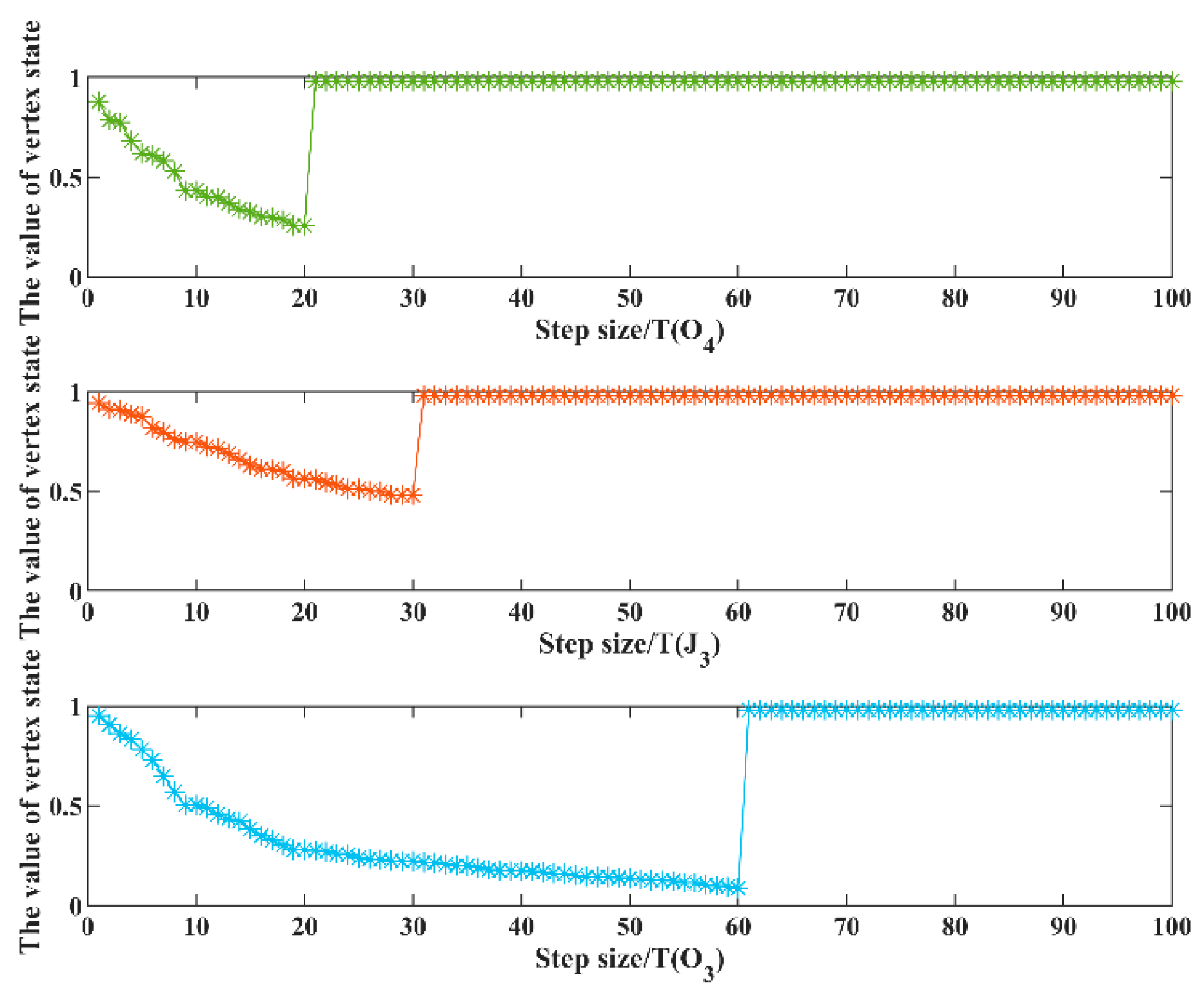
The brittleness evolution model of the supply chain without considering the vertex adaptability is simulated. The brittleness evolution curve of the vertex state is shown in Figure 2.

As shown in Figure 2, when the vertex adaptability is not considered, O₄ immediately fails, whose vertex state reaches the peak value. This is because the brittle link between O₄ and I₃ is close. The brittleness of O₄ is stimulated after being disturbed by the collapse of I₃.

The reason is, when the vertex which has a brittle link with the brittle source, such as I₃, is suddenly disturbed, its entropy increases abruptly. In order to maintain the original state, the vertex will absorb the negative entropy flow from the adjacent subsystem. However, the negative entropy cannot cope with such brittleness disturbance, which is strong and sudden. Therefore, the vertex collapses.

The entropy of the adjacent vertex, which provides negative entropy, increases sharply, and it would also collapse after a period of time. The whole supply chain system eventually suffers the brittleness collapse.

Moreover, in Figure 2, the vertex should go through $n$ states including $x_i^0$,${ x}_i^1$, $x_i^2$, …, $x_i^n$ to collapse after being suffered from the brittleness interference. Therefore, the vertex brittleness of the supply chain has the feature of time delay.

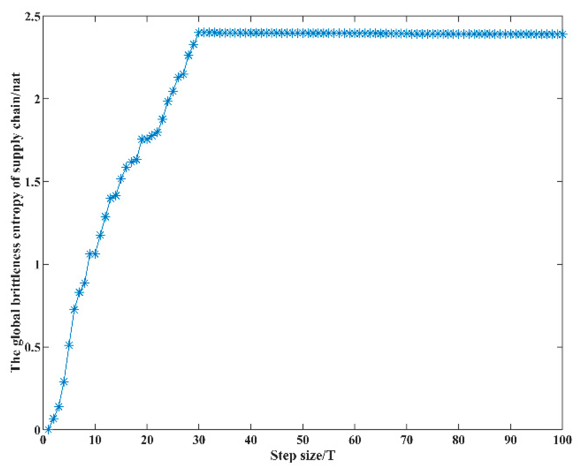
When the vertex adaptability is not considered, the evolution curve of the global brittleness entropy of the supply chain is shown in Figure 3.

As is shown in Figure 3, when the vertex adaptability is not considered, the global brittleness entropy of the supply chain reaches the peak when the step size is 30. This indicates that the degree of global disorder of the supply chain is greatly affected by the systematical collapse behavior. This is because, when the global entropy of brittleness reaches the critical value, the propagation speed of brittleness behavior is very fast. And there is no link between the vertex of brittleness source and the main vertexes of the supply chain.

In Figure 2 and Figure 3, we can see that the collapse behavior of vertex has great influence on the degree of global disorder on the supply chain. The more vertexes collapsed, the much closer the global brittleness entropy is to the critical value.

Meanwhile, we can also find that it takes a period of time for the whole supply chain system to collapse completely. This is because the collapse time of the system mainly depends on the capacity of the anti-brittleness of the vertex, that is to say, depending on its negative entropy value, which reflects the relationship of the non-cooperative game between vertexes of the supply chain.

6.3. Brittleness Evolution Simulation When Vertex Adaptability Is Considered

The brittleness evolution model of the supply chain considered the vertex adaptability was simulated, and the evolution curves of the brittleness entropy value are shown in Figure 4.

As is shown in Figure 4, when the vertex adaptability is considered, O₄ does not collapse immediately after being disturbed by the vertex of the brittleness source but collapses when the step size is 100 T. Then, both the vertex state value and the brittleness entropy reach the thresholds. This is due to the adaptive behavior of vertexes.

The state value and the threshold of vertex J₃ and O₃ fluctuated around a certain equilibrium value but never reached the threshold of brittleness. This is because vertexes have the adaptability to analyze the state of their own and the surrounding environment. Then, the adaptive vertexes make a decision as follows: They choose to quit the competition when the negative entropy of resources of the environment are not sufficient, and the vertexes are not on the edge of brittleness collapse. When the negative entropy of resources of the environment are sufficient, not only would the entropy production of the whole supply chain system be reduced, but also that of the vertex will be reduced, which makes the vertex further from the brittleness state.

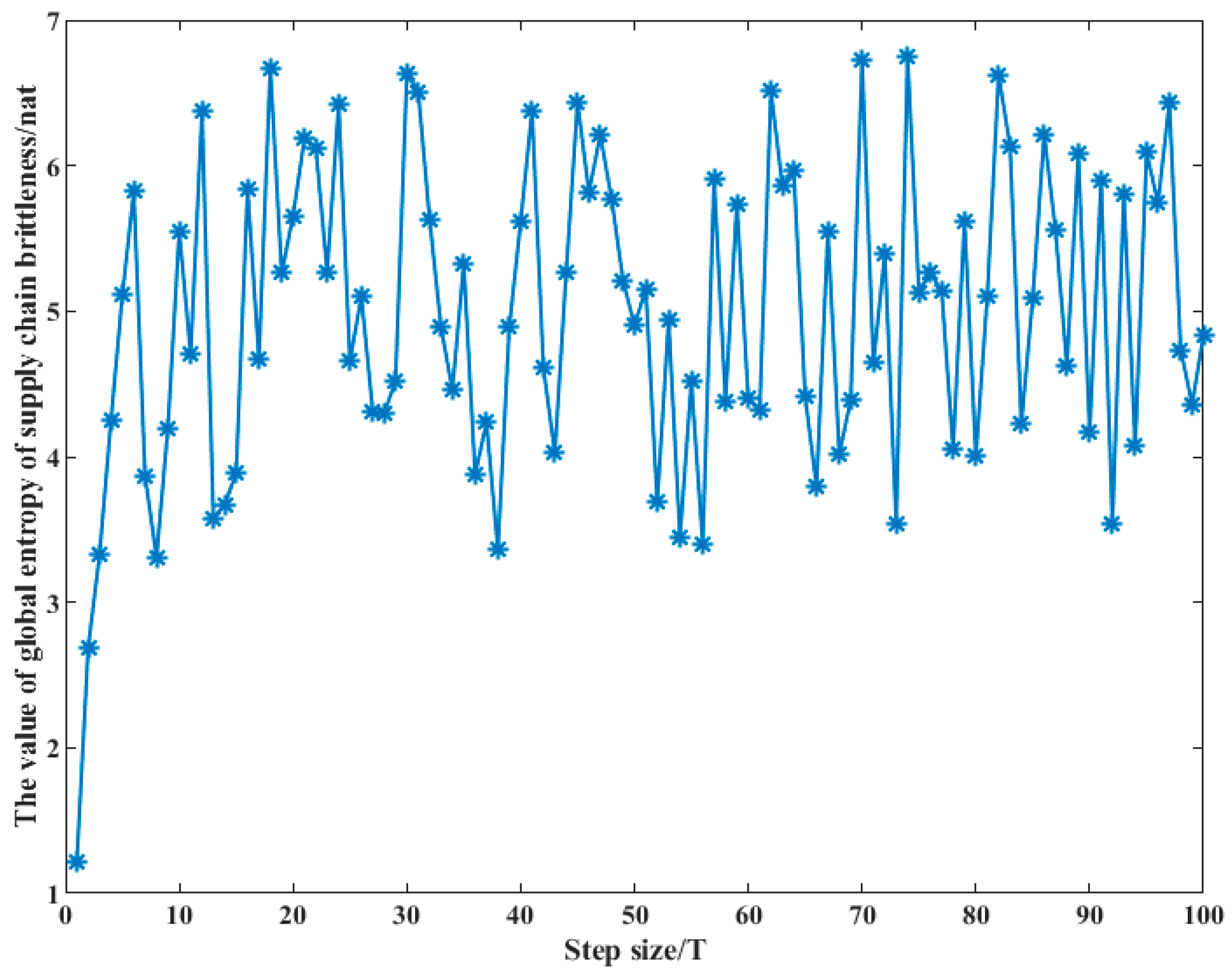
When the vertex adaptability is considered, the evolution curve of the global brittleness entropy is shown in Figure 5.

As is shown in Figure 5, the global brittleness entropy increases rapidly at the beginning and then presents a state of periodic oscillation, the oscillation amplitude of which tends to be stable. This is because the adaptive behavior of the vertex agent resists the brittleness evolution of the supply chain to collapse.

In Figure 4 and Figure 5, we found that the adaptive behavior of the supply chain vertex can protect the operation order of the system, in which it avoids the brittleness collapse of each vertex or delays the brittleness collapse when the system is disturbed by the COVID-19 pandemic. Therefore, the adaptive behavior of each vertex has a certain purpose.

In addition, if the vertex has such adaptive behavior, the negative entropy flow must be input, and the vertex has a cooperative game relationship with others. Therefore, in supply chain management, the adaptability of each vertex should be enhanced, which is a measure of the enterprise to prevent brittleness or reduce the effect of brittleness.

6.4. Evolution Simulation Considered Characteristics of Seasonal Demand of the Supply Chain

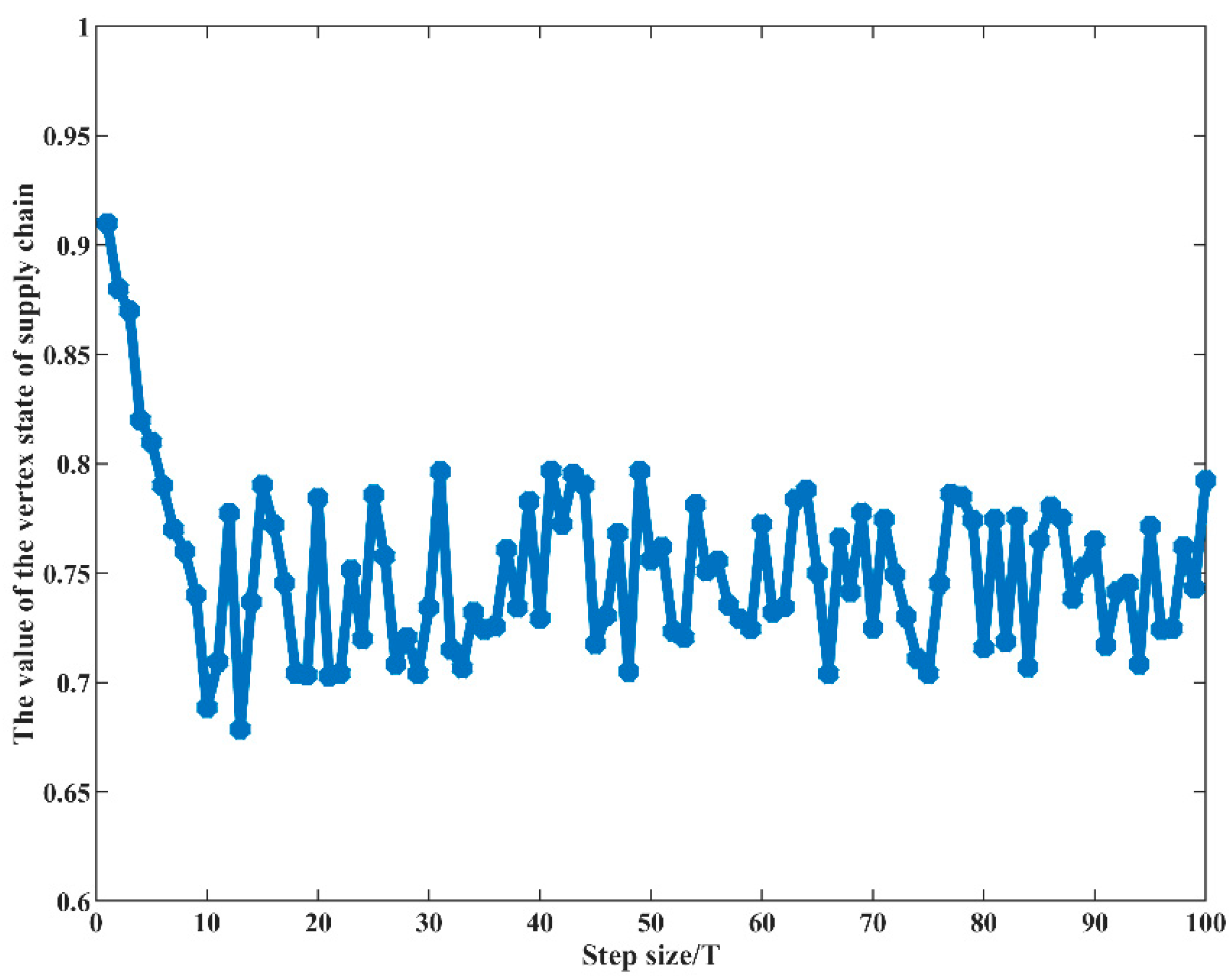
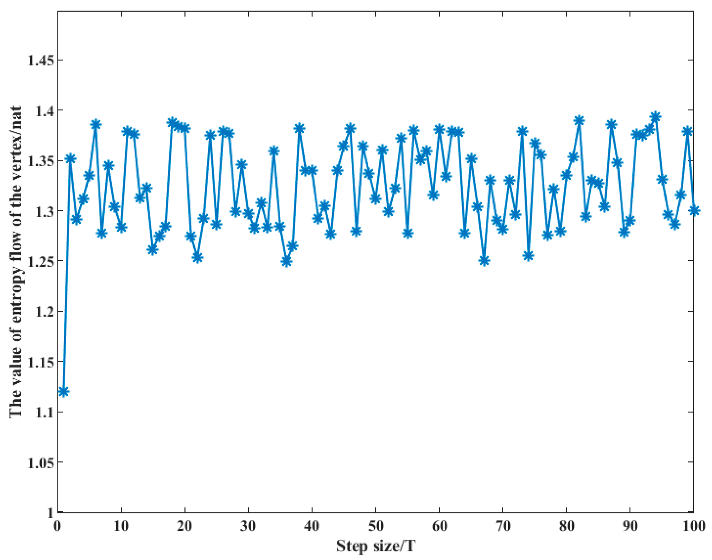
The scheduling schemes of the supply chain under the demand scenarios P_m = 0.3 (the scenario of the peak season) and P_m = 0.2 (the off-season scenario) are calculated, respectively, when I₃ is the brittleness source [45]. The brittleness evolution model of the supply chain considering the vertex adaptability was simulated. And the evolution curves of the vertex state and entropy flow of O₂ in peak season are shown in Figure 6 and Figure 7, respectively. The evolution curves of the entropy flow of O₂ and the global brittleness entropy of the supply chain are, respectively, shown in Figure 8 and Figure 9.

In Figure 6 and Figure 7, both the value of the vertex state and that of the entropy flow approach the collapse threshold in the peak season. In Figure 9, the global brittleness entropy of the supply chain oscillates up and down around a certain value with a large amplitude, and the entropy value is much larger than that in the off-season and other normal seasons. Therefore, the brittleness of the supply chain in the peak season is more likely to be stimulated than that in the off-season and other normal seasons, and the prediction is more difficult in the peak season.

In Figure 8, although the entropy flow value of the vertex is far from the collapse threshold in the off-season, the amplitude of the curve of brittleness evolution is large. In Figure 9, it can also be found that, although the value of the global entropy flow is small, the amplitude of the curve is large. this indicates that the possibility that brittleness is stimulated in the off-season varies widely, and the prediction of brittleness is difficult.

Therefore, the supply chain is prone to collapse in the peak season, and its brittleness has been kept in a state that is easier to be triggered. The brittleness of the supply chain system is difficult to predict in other seasons. The operation and management departments should take measures to avoid shortages to prevent the system from collapsing.

6.5. The Evolution Simulation of Brittleness Behavior

Based on the supply chain scheduling schemes under the demand scenario of P_m = 0.5 [45], in which λ_D was used to divide scheduling schemes into three main categories, to whose link weight ω_ij the brittleness collapse scenarios corresponding are, respectively, λ_D > 0, λ_D = 0, λ_D < 0. The results of these three kinds of scheduling schemes are taken as the initial data of brittleness evolution. The evolution curves of global brittleness entropy of the supply chain network with different λ_D are shown in Figure 10, Figure 11 and Figure 12, respectively.

In Figure 10, λ_D = 0 represents the first kind of brittleness behavior, in which the curve of the global brittleness entropy randomly oscillated, and the amplitude is uncertain. Therefore, the first kind of brittleness behavior is unpredictable. As the value of the brittleness entropy is not large, the brittleness of the supply chain is not prone to being triggered. The randomness of brittleness events increases, so the difficulty of the brittleness control increases in the first kind of brittleness behavior.

As is shown in Figure 11, λ_D > 0 represents the second kind of brittleness behavior, in which the curve of the global brittleness entropy reaches a stable value in a short time, and the oscillation time is short. If the brittleness source can cause the collapse of the whole supply chain, the speed of the brittleness evolution would be very fast, and brittleness would spread quickly throughout the whole network. Meanwhile, this kind of brittleness behavior is more predictable.

In Figure 12, λ_D < 0 represents the third kind of brittleness behavior, the amplitude of the curve of which is larger than that of the second kind of brittleness behavior. Therefore, the stability of the system of the third brittleness behavior is inferior to that of the second one. As the curve of the global brittleness entropy also oscillates randomly, the third kind of brittleness behavior is difficult to predict, and the value of the brittleness entropy is relatively large, so the brittleness is prone to being triggered. As the brittleness behavior is difficult to predict, it is very difficult to manage and control the brittleness of the supply chain.

7. Conclusions and Future Research

In this paper, the problem of the brittleness evolution of the supply chain under attack from the COVID-19 pandemic was studied. In contrast to the previous research of the evaluation study on “supply chain vulnerability”, we introduced the concept of “supply chain brittleness” in this study, which was biased towards a physical concept. And the collapse property and evolution law of the supply chain under external attack were quantitatively studied.

Based on the adaptive agent graph theory, the brittleness evolution model in which the vertex adaptability was considered and was not considered, respectively, was constructed, and the simulation algorithm, in which was the scheduling model of the uncertain supply chain, was taken as the auxiliary technology element. The effectiveness of the model and algorithm was proved by a numerical simulation of an electronic supply chain. Findings are listed as follows.

• Brittleness evolution law based on the vertex adaptability of the supply chain

  (1)

  When the vertex adaptability is not considered, the supply chain system does not collapse immediately when the vertex of the brittleness source is failed but takes a certain period of time, which reflects the feature of delay of the supply chain’s brittleness.

  (2)

  When the vertex adaptability is considered, the vertex which has a close brittleness link with the brittleness source does not immediately collapse. This is because the adaptive behavior of the vertex agent resists the brittleness evolution of the supply chain to collapse.

• Seasonal evolution law of supply chain brittleness based on demand characteristics

The brittleness of the supply chain in peak season is more likely to be stimulated than that in the off-season and other normal seasons. Therefore, the operational and management departments of the enterprise should take measures to avoid shortages to prevent the system from crashing.

3.

The evolution law of brittleness behavior of the supply chain

The value of brittleness entropy of the first kind of brittleness behavior is not large, so the brittleness of the supply chain is not prone to being triggered; by contrast, the second kind of brittleness behavior is not difficult to predict, and the speed of the brittleness evolution would be very fast; the third kind of brittleness behavior is difficult to predict, which is the most difficult in management and control of the supply chain brittleness.

In this paper, the brittleness theory of complex systems is applied to study the mechanism of interruption and collapse of the supply chain, which has certain theoretical value. The brittleness theory of complex systems has become mature during the development of nearly 20 years. This theory can explain well the actual phenomenon that the collapse of one single element in a complex system leads to the collapse of the whole system. In recent years, the brittleness theory has been widely used in the area of electric power, the coal sector, transportation, and other fields. However, it is rarely applied and verified in the field of supply chain security. Based on the adaptive agent graph theory, we studied the mechanism of disruption and collapse of the supply chain from the perspective of the brittleness of complex systems, which not only enriched the connotation of brittleness theory but also broadened the research perspective of the issue on supply chain security.

In practice, it is of great significance for management of supply chain security to study the evolution law of supply chain brittleness based on vertex adaptability. To keep the adaptability of vertexes, enterprises should adopt various policies and measures to ensure the input of the negative entropy flow of vertexes, and the relationship of the cooperative game with other vertexes should be established. Only by ensuring the adaptability of each participant of the supply chain can enterprises prevent the interruption and collapse of the supply chain and combat the brittleness property of the supply chain.

The limitations of this study and questions to be further studied are as follows:

• The model constructed in this paper is only considered the characteristics of the vertex within the supply chain system, based on which the brittleness evolution of the supply chain is compared and analyzed. The COVID-19 pandemic outside the supply chain system has attacked and disrupted the supply chain to varying degrees; therefore, the attack of the COVID-19 pandemic can be modeled and quantified to study its impact on the brittleness evolution of the supply chain in the future.
• The characteristics of the seasonal demand of brittleness evolution of the supply chain are compared and analyzed in this paper. In the future, more cluster analysis of demand characteristics can be conducted to study the relationship between brittleness evolution and more demand characteristics.

References

1. Xu, N.R.; Liu, J.B.; Li, D.X.; Wang, J. Research on Evolutionary Mechanism of Agile Supply Chain Network via Complex Network Theory. Math. Probl. Eng. 2016, 2016, 4346580. [Google Scholar] [CrossRef]
2. Yamin, M.A. Investigating the Drivers of Supply Chain Resilience in the Wake of the COVID-19 Pandemic: Empirical Evidence from an Emerging Economy. Sustainability 2021, 13, 11939. [Google Scholar] [CrossRef]
3. Sombultawee, K.; Lenuwat, P.; Aleenajitpong, N.; Boon-itt, S. COVID-19 and Supply Chain Management: A Review with Bibliometric. Sustainability 2022, 14, 3538. [Google Scholar] [CrossRef]
4. Moyano-Fuentes, J.; Bruque-Camara, S.; Maqueira-Marin, J.M. Development and validation of a lean supply chain management measurement instrument. Prod. Plan. Control 2019, 30, 20–32. [Google Scholar] [CrossRef]
5. Rivera-Gomez, H.; Medina-Marin, J.; Santana-Robles, F.; Montano-Arango, O.; Barragan-Vite, I.; Cisneros-Flores, G. Impact of Unreliable Subcontracting on Production and Maintenance Planning Considering Quality Decline. Appl. Sci. 2022, 12, 3379. [Google Scholar] [CrossRef]
6. Golan, M.S.; Mahoney, E.; Trump, B.; Linkov, I. Resilience and efficiency for the nanotechnology supply chains underpinning COVID-19 vaccine development. Curr. Opin. Chem. Eng. 2021, 34, 100759. [Google Scholar] [CrossRef]
7. Elwood, A. Supply chain resilience. J. Bus. Contin. Emerg. Plan. 2021, 15, 65–77. [Google Scholar]
8. Nakatani, J.; Tahara, K.; Nakajima, K.; Daigo, I.; Kurishima, H.; Kudoh, Y.; Matsubae, K.; Fukushima, Y.; Ihara, T.; Kikuchi, Y.; et al. A graph theory-based methodology for vulnerability assessment of supply chains using the life cycle inventory database. Omega-Int. J. Manag. Sci. 2018, 75, 165–181. [Google Scholar] [CrossRef]
9. Sharma, S.K.; Routroy, S.; Singh, R.K.; Nag, U. Analysis of supply chain vulnerability factors in manufacturing enterprises: A fuzzy DEMATEL approach. Int. J. Logist.-Res. Appl. 2022, 20, 83590. [Google Scholar] [CrossRef]
10. Blackhurst, J.; Rungtusanatham, M.J.; Scheibe, K.; Ambulkar, S. Supply chain vulnerability assessment: A network based visualization and clustering analysis approach. J. Purch. Supply Manag. 2018, 24, 21–30. [Google Scholar] [CrossRef]
11. Wagner, S.M.; Neshat, N. Assessing the vulnerability of supply chains using graph theory. Int. J. Prod. Econ. 2010, 126, 121–129. [Google Scholar] [CrossRef]
12. Karwasra, K.; Soni, G.; Mangla, S.K.; Kazancoglu, Y. Assessing dairy supply chain vulnerability during the COVID-19 pandemic. Int. J. Logist.-Res. Appl. 2021. [Google Scholar] [CrossRef]
13. Ekanayake, E.; Shen, G.Q.; Kumaraswamy, M.; Owusu, E.K. Critical supply chain vulnerabilities affecting supply chain resilience of industrialized construction in Hong Kong. Eng. Constr. Archit. Manag. 2021, 28, 3041–3059. [Google Scholar] [CrossRef]
14. Sharma, S.K.; Srivastava, P.R.; Kumar, A.; Jindal, A.; Gupta, S. Supply chain vulnerability assessment for manufacturing industry. Ann. Oper. Res. 2021. [Google Scholar] [CrossRef]
15. Majumdar, A.; Sinha, S.K.; Shaw, M.; Mathiyazhagan, K. Analysing the vulnerability of green clothing supply chains in South and Southeast Asia using fuzzy analytic hierarchy process. Int. J. Prod. Res. 2021, 59, 752–771. [Google Scholar] [CrossRef]
16. Liu, J.G.; Liu, F.; Zhou, H.; Kong, Y.D. An Integrated Method of Supply Chains Vulnerability Assessment. Sci. Program. 2016, 2016, 2819238. [Google Scholar] [CrossRef]
17. Naghshineh, B.; Carvalho, H. The implications of additive manufacturing technology adoption for supply chain resilience: A systematic search and review. Int. J. Prod. Econ. 2022, 247, 108387. [Google Scholar] [CrossRef]
18. Ruel, S.; Shaaban, S.; Ducros, M. Supply chain vulnerability: Contributions from an edifying case study. J. Enterp. Inf. Manag. 2019, 32, 214–232. [Google Scholar] [CrossRef]
19. Bassett, H.R.; Sharan, S.; Suri, S.K.; Advani, S.; Giordano, C. A comparative study of small-scale fishery supply chains’ vulnerability and resilience to COVID-19. Marit. Stud. MAST 2022, 21, 173–192. [Google Scholar] [CrossRef]
20. Viljoen, N.M.; Joubert, J.W. The Road most Travelled: The Impact of Urban Road Infrastructure on Supply Chain Network Vulnerability. Netw. Spat. Econ. 2018, 18, 85–113. [Google Scholar] [CrossRef]
21. Saengchai, S.; Jermsittiparsert, K. The mediating role of supplier network, the moderating role of flexible resources in the relationship between lean manufacturing practices and the organizational performance. Humanit. Soc. Sci. Rev. 2019, 7, 720–727. [Google Scholar] [CrossRef] [Green Version]
22. Ma, F.; Xue, H.F.; Yuen, K.F.; Sun, Q.P.; Zhao, S.M.; Zhang, Y.X.; Huang, K. Assessing the Vulnerability of Logistics Service Supply Chain Based on Complex Network. Sustainability 2020, 12, 1991. [Google Scholar] [CrossRef]
23. Wagner, S.M.; Neshat, N. A comparison of supply chain vulnerability indices for different categories of firms. Int. J. Prod. Res. 2012, 50, 2877–2891. [Google Scholar] [CrossRef]
24. Shughrue, C.; Seto, K.C. Systemic vulnerabilities of the global urban-industrial network to hazards. Clim. Change 2018, 151, 173–187. [Google Scholar] [CrossRef]
25. Kurniawan, R.; Zailani, S.H.; Iranmanesh, M.; Rajagopal, P. The effects of vulnerability mitigation strategies on supply chain effectiveness: Risk culture as moderator. Supply Chain Manag.-Int. J. 2017, 22, 1–15. [Google Scholar] [CrossRef]
26. Bai, H.X.; Ran, W.X. Analysis of the Vulnerability and Resilience of the Tourism Supply Chain under the Uncertain Environment of COVID-19: Case Study Based on Lijiang. Sustainability 2022, 14, 2571. [Google Scholar] [CrossRef]
27. Zhang, H.; Jia, F.; You, J.X. Striking a balance between supply chain resilience and supply chain vulnerability in the cross-border e-commerce supply chain. Int. J. Logist.-Res. Appl. 2021. [Google Scholar] [CrossRef]
28. Guo, J.; Wu, D.J. Qualitative Analyzing Brittleness of Complex System Based on Catastrophe Theory. In Proceedings of the 20th Chinese Control and Decision Conference, Yantai, China, 2–4 July 2008. [Google Scholar]
29. Guo, J.; Wu, D.J. Researching the Brittleness of Traffic System Based on Cusp Catastrophe Model. In Proceedings of the IEEE International Conference on Automation and Logistics, Qingdao, China, 1–3 September 2008. [Google Scholar]
30. Guo, J.; Chen, X.L.; Jin, H.Z.; Wu, D.J. Analyzing brittleness of complex system based on the catastrophe theory. In Proceedings of the 2007 International Conference on Intelligent Systems and Knowledge Engineering, Chengdu, China, 15–16 October 2007. [Google Scholar]
31. Guo, J.; Wu, D.J. Based on the relation of evolution among systems to analyze brittleness of complex system. In Proceedings of the 6th World Congress on Intelligent Control and Automation, Dalian, China, 21–23 June 2006. [Google Scholar]
32. Guo, J.; Wu, D.J. Based on cusp catastrophe potential function to analyze brittleness of complex system. In Proceedings of the Chinese Control Decision Conference, Guangzhou, China, 3–6 July 2007. [Google Scholar]
33. Wei, Q.; Jin, H.Z.; Ji, M. The research on brittle catastrophe of complex giant system. In Proceedings of the IEEE Region 10 Technical Conference on Computers, Communications, Control and Power Engineering, Beijing, China, 28–31 October 2002. [Google Scholar]
34. Guo, J.; Li, W.C.; Wu, D.J. Research on the brittleness of complex system based on brittleness potential function. In Proceedings of the IEEE International Conference on Systems, Man and Cybernetics, The Hague, The Netherlands, 10–13 October 2004. [Google Scholar]
35. Wei, Q.; Jin, H.Z.; Guo, J.; Ji, M. Research on the complex system based on the brittle characteristic. In Proceedings of the SICE 2003 Annual Conference, Fukui, Japan, 4–6 August 2003. [Google Scholar]
36. Cao, R.; Jin, H.Z. Brittleness Analysis of Complex Systems Subject to Cascading Failure. In Proceedings of the 10th IEEE International Conference on Mechatronics and Automation (ICMA), Takamatsu, Japan, 4–6 August 2013. [Google Scholar]
37. Wei, Q.; Wei, X.L.; Jin, H.Z. Brittleness theory and its application on the analysis of SARS. In Proceedings of the 6th World Congress on Intelligent Control and Automation, Dalian, China, 21–23 June 2006. [Google Scholar]
38. Wei, Q.; Jin, H.Z.; Guo, J.; Ji, M. Study on complex system based on the brittleness. In Proceedings of the IEEE International Conference on Systems, Man and Cybernetics (SMC 03), Washington, DC, USA, 5–8 October 2003. [Google Scholar]
39. Yan, L.M.; Jin, H.Z.; Xu, J.J.; Wang, Q.; Rong, P.X. Analysis of brittleness in complex electric power systems. In Proceedings of the 17th Chinese Control and Decision Conference, Harbin, China, 25–27 June 2005. [Google Scholar]
40. Jin, H.Z.; Yan, L.M.; Rong, P.X.; Liu, X.B.; Li, M.D. Brittleness analysis of electric network. Dyn. Contin. Discret. Impulsive Syst. -Ser. B-Appl. Algorithms 2005, 1, 32–36. [Google Scholar]
41. Wu, H.M.; Jin, H.Z. Analysis of brittle tree of complex system based on chart theory. In Proceedings of the 21st Chinese Control and Decision Conference, Guilin, China, 17–19 June 2009. [Google Scholar]
42. Wang, J.; Zhu, X.Y.; Hu, X.W. Research on the Evaluation Methods of Highway Traffic System Brittle Source. In Proceedings of the 5th International Conference on Intelligent Systems Design and Engineering Applications (ISDEA), Zhangjiajie, China, 15–16 June 2014. [Google Scholar]
43. Lin, D.M.; Jin, H.Z.; Xue, P.; Wu, H.M.; Wang, H. Research on brittleness of traffic system based on adaptive agent digraph. J. Syst. Simul. 2008, 20, 733–737. [Google Scholar]
44. Yan, W. Study of supply chain’s brittleness based on the complex system brittle theory. In Proceedings of the IEEE International Conference on Grey Systems and Intelligent Services, Nanjing, China, 18–20 November 2007. [Google Scholar]
45. Cao, W.; Wang, X.F. A Multiobjective Multiperiod Mixed-Integer Programming Optimization Model for Integrated Scheduling of Supply Chain Under Demand Uncertainty. IEEE Access 2022, 10, 63958–63970. [Google Scholar] [CrossRef]
46. Holland, J.H. Complex Adaptive Systems. Daedalus 1992, 121, 17–30. [Google Scholar]
47. Lin, D.M.; Jin, H.Z.; Wu, H.M.; Xue, P.; Wang, H. Research on brittleness of complex systems based on ant colony algorithm. Syst. Eng. Electron. 2008, 30, 743–747. [Google Scholar]
48. Wang, A.J.; Lin, G.L.; Wang, X.Q. Research on the Model of Hazardous Material Transport System’s Brittle Risk. In Proceedings of the International Conference of Management Engineering and Information Technology, Zhengzhou, China, 17–18 October 2009. [Google Scholar]
49. Jiang, Z.; Pan, X.; Lin, Y. Risk analysis of equipment system-of-systems architecture based on entropy and brittleness. In Proceedings of the 26th Conference on European Safety and Reliability (ESREL), Glasgow, Scotland, 25–29 September 2016. [Google Scholar]
50. Zhou, J.B.; Dong, S.; Yan, B.; Zhang, M.J.; Yang, R.F. An adaptive agent digraph simulation for road traffic safety statue in bridge-tunnel groups. Adv. Mech. Eng. 2017, 9, 1687814017715979. [Google Scholar] [CrossRef]
51. Yang, J.X.; Zhou, J.T.; Han, F.Q. Study on State Recognition of ASCE Benchmark FEM based on Lyapunov Exponent Spectrum Entropy. In Proceedings of the International Conference on Applied Mechanics, Materials and Manufacturing (ICAMMM 2011), Shenzhen, China, 18–21 November 2011. [Google Scholar]
52. Gao, X.Y.; Zhao, Y.; Wang, Y.H.; Zuo, X.; Chen, T. A Lagrange Relaxation Based Decomposition Algorithm for Large-Scale Offshore Oil Production Planning Optimization. Processes 2021, 9, 1257. [Google Scholar] [CrossRef]
Figure 1. Supply chain network topology diagram of electronic product with two-layer time.
Sustainability 14 12211 g001
Figure 2. Brittleness evolution graph of the vertex state of uncertain supply chain without considering the vertex adaptability (γ = 0.5, Pm = 0.5, I3 is the brittleness source).
Sustainability 14 12211 g002
Figure 3. Brittleness evolution graph of the global entropy of uncertain supply chain without considering the vertex adaptability (γ = 0.5, Pm = 0.5, I3 is the brittleness source).
Sustainability 14 12211 g003
Figure 4. Brittleness evolution graph of the entropy flow of vertexes considering the vertex adaptability (γ = 0.5, Pm = 0.5, I3 is the brittleness source).
Sustainability 14 12211 g004
Figure 5. Brittleness evolution graph of the global entropy of uncertain supply chain considering the vertex adaptability (γ = 0.5, Pm = 0.5, I3 is the brittleness source).
Sustainability 14 12211 g005
Figure 6. Brittleness evolution graph of vertex state of uncertain supply chain in peak season (γ = 0.5, Pm = 0.5, I3 is the brittleness source).
Sustainability 14 12211 g006
Figure 7. Brittleness evolution graph of entropy flow of the vertex in peak season (γ = 0.5, Pm = 0.5, I3 is the brittleness source).
Sustainability 14 12211 g007
Figure 8. Brittleness evolution graph of entropy flow of the vertex in peak season (γ = 0.5, Pm = 0.5, I3 is the brittleness source).
Sustainability 14 12211 g008
Figure 9. Seasonal evolution curves of the global brittleness entropy of uncertain supply chain (γ = 0.5, I3 is the brittleness source).
Sustainability 14 12211 g009
Figure 10. The evolution graph of the first kind of brittleness behavior of uncertain supply chain network (γ = 0.5, Pm = 0.5, λD = 0).
Sustainability 14 12211 g010
Figure 11. The evolution graph of the second kind of brittleness behavior of uncertain supply chain network (γ = 0.5, Pm = 0.5, λD > 0).
Sustainability 14 12211 g011
Figure 12. The evolution graph of the third kind of brittleness behavior of uncertain supply chain network (γ = 0.5, Pm = 0.5, λD < 0).
Sustainability 14 12211 g012