Investigating the Mediating Roles of Income Level and Technological Innovation in Africa’s Sustainability Pathways Amidst Energy Transition, Resource Abundance, and Financial Inclusion

Abstract

The global environment faces the issue of sustainability arising from the persistent growth rates in general production levels. Hence, there is the need to resolve the growth environment conflicts in order to enhance the sustainability of the current and future generations. This study presents the first empirical analysis on the dynamic impacts of non-renewable and renewable energy, total resource rents, population growth, human capital, and financial inclusion on environmental quality in Sub-Saharan Africa (SSA) with the conditioning roles of technological progress and income level. The empirical evidence is based on a two-step system generalized method of moments (SYS-GMM) with forward orthogonal deviations for 42 countries in the SSA region from 2004 to 2018. The following results are established from the empirical analyses. First, renewable energy emerges as a promoter of environmental quality through its reducing impacts on carbon emissions per capita (co2pc). Second, other regressors turn out to impede environmental quality by contributing to the surge in co2pc. Third, the robustness checks analyses, which consider different variants of carbon emissions as outcome variables, revealing that the main results are robust and empirically supported to explain the variations in the level of pollutants in the region. Fourth, the impacts of technological progress from both direct (unconditional) and interactive (conditional) angles mitigate co2pc while income promotes it. On the policy front, promoting investment in renewable energy and structuring human capital development plans to promote green growth are seen as sacrosanct towards achieving a sustainable environment in the region.

1. Introduction

The need to resolve the pervasive threats posed by environmental pollution has attracted growing interest among research pundits, policymakers, and international organizations alike. This concern has subsequently motivated the emerging advocacies on the necessity of improving the quality of the environment across all levels of economic interactions, from the global down to the national [1]. The concerns about the ecosystem are based on the inevitable need to take cautious actions on the consequences of human economic and non-economic activities, particularly as they pose the irreparable loss on the present and future sustainability of the environment. The preceding narrative has stirred the emergence of numerous international treaties from the late 1990s to the recent times (a few of these include; the United Nations Framework Convention on Climate Change (UNFCCC) in 1992, the Kyoto Protocol of 1997, Sustainable Development Goals (SDGs) of 2015, and the 24th and 21st editions of the conference of the parties (COP24 and COP21) in 2018 and 2015, respectively). The central objective of these treaties and several others is to achieve a benchmark reduction in carbon emissions reported to have recorded a persistent rise of 1.5% with a peak record of 37.5 37.5 GtCO2 yearly [2].

Despite the various global efforts aimed at ending the challenge of the diminishing quality of the environment, the issue remains persistent, thereby motivating scores of research tailored towards unravelling the drivers of environmental equality. The prominent factors that have surfaced so far include energy consumption [3,4] institutions, and regulatory pressure [5,6], trade openness [7], forest and mineral volatility [8] urbanization [9], financial development [10], economic growth [11], poverty and logistics operation [12], biomass energy [13] and foreign direct investment [14]. That notwithstanding, it is pertinent to note that research explicating the environmental effects of other factors, such as total resource rents, population growth, human capital, and financial inclusion are just evolving. The evolving nature of empirical studies on the highlighted factors allows the present study to extend the frontier of knowledge, especially in emerging regions such as Sub-Saharan Africa (SSA), where the highlighted factors of concern are prominent development indicators. In justifying the consideration for the role of natural resource rents, it is pertinent to note that the revenues generated from the exploration of natural resources have put policymakers at indecision on the action to be taken in the interest of the environment [15]. The standard hypothesis held in the literature has often been based on the possibility of investing revenues earned from natural resources in a way that will effectively decarbonize the environment [16]. Nonetheless, the net impacts of the carbon emitted during the exploration period remain an issue of contention. By implication, natural resource rents can either reduce (increase) the level of carbon emissions subject to the efficient (inefficient) utilization of the earnings received. Further, the potential environmental effects of population growth are not negligible. The reason is that anthropogenic activities regarded as significant sources of carbon emissions directly link with population growth [17]. In such a case, an increase in population leads to a corresponding increase in carbon emissions. Corroborating this assertion, Ref. [18] posits that a rise in population would trigger a corresponding increase in consumption of energy resources with an eventual rise in carbon emissions in the coming decades.

Furthermore, the environmental impacts of human capital have been argued from two standpoints. The first strand involves a group of emerging empirical studies which argued that human capital leads to a significant increase in carbon emissions [14,19]. In particular, [20] opine that high energy consumption that will enhance human capital development should be the priority of any country aiming to achieve sustainable economic growth. In such a case, both energy consumption and carbon emissions increase concurrently. The second standpoint argues that human capital lessens the stock of environmental pollutants [21].

Regarding the environmental impacts of financial inclusion, empirical findings on the nexus have provided mixed reactions [11]. At one point, some view that financial inclusion avails both businesses and household consumers the financial capacity to afford green technology and adhere to all stipulated environmental standards, which in a way help reduce greenhouse gas emissions [22]. Contrarily, others aver that accessibility to financial services may encourage manufacturing and industrial companies to increase their production activities, leading to an increase in carbon emissions [23]. Following these contravening standpoints, financial inclusion can serve as a deterrent or stimulus to carbon emissions.

Going by the above expositions on the highlighted variables of concern, it is evident that the environmental effects of these explicated variables, despite their emerging interest in the literature, have not received a decisive stand. This lack of clarity and consensus suggests that more is still desired, especially in developing regions such as SSA. Moreover, the modulating role of technology in the environment-growth nexus has remained less debated in SSA despite the theoretical evidence advancing its importance. In addition, empirical evidence explaining how income level intermediate in the environmental quality debates is scarcely available. These two loopholes may explain some of the reasons for the inherent inconclusiveness and the observed controversies among the existing studies leading to policy failure in addressing environmental degradation globally, particularly in SSA.

Research Objective/Contributions

There is no gainsaying that the SSA region is facing devastating threats from environmental degradation. This environmental tragedy is further complicated by the unfolding challenges of global warming, of which SSA is the most vulnerable. In view of this, the prime focus of the research paper is to probe the dynamic effects of renewable and non-renewable energy, total resource rents, population growth, human capital, and financial inclusion on environmental quality in SSA with the conditioning role of technology and income level. The SSA region remains an elected candidate for at least four reasons. First, empirical studies have advanced that environmental degradation remains an issue of concern in SSA with impending threats of global warming [24,25]. Available reports reveal that, despite SSA contributing insignificantly to the global volume of carbon emissions behind China, Russia, India, and Japan, the region has witnessed a remarkable rise in carbon emissions more than twelve times since the 1950s [26]. More worrisome, existing reports show that SSA is endangered by climate change, thus making the region among the most susceptible to it [27]. Second, in the past few decades, the population size of the SSA region has grown at an average rate of 2.5% and is forecasted to double by 2036 [28]. In recent times, the population growth has maintained an annual increase of 2.7%, which is two times more than South Asia (1.2%) and Latin America (0.9%) regions [29]. In particular, the SSA region is anticipated to house more than half of the global population between 2019 and 2050, with an expected increase of 1.05 billion people [30]. The population increase in SSA has significant implications for the region’s environment, which necessitates the need for an inquiry into it. Third, there are emerging facts attesting to the various economic resurgences in SSA, which have led to some remarkable improvements in the performance of the region’s economy [1]. This performance has subsequently seen countries in the region emerge top in the list of rapidly growing economies globally [2]. Fourth, information computer technology (ICT) in SSA has recorded unprecedented successes recently [31]. That notwithstanding, empirical evidence shows that the progress recorded so far are still at the early phase [32], suggesting that good days lie ahead for the region in the ICT sector. Consequent upon evidence advancing the thriving moments for economic performance and technology in the SSA region, assessing the extent to which these two indicators can contribute to addressing the region’s environmental tragedy becomes highly fundamental and sacrosanct for the achievements of sustainable development goals 2030 and African Agenda 2063. This inquiry constitutes one of the primary motivations of this study.

This paper extends the frontier of knowledge in the environmental determinants literature in at least five ways. First, the results emanating from the existing empirical studies on the environmental impacts of energy consumption have remained inconclusive and mixed, thus leaving the door open for research of this nature. Second, a detailed assessment of the existing studies reveals little about the environmental consequence of variables, e.g., total resource rents, population growth, human capital, and financial inclusion in SSA, despite their growing importance and contribution to the region’s environment. This study will constitute the first strand of empirical efforts examining the dynamic effects of these variables on environmental quality in SSA. Third, the mediating role of income level between carbon emissions and the drivers above is yet another scantly debated area, notwithstanding the giant economic strides SSA is recording. Following the theoretical proposition advanced by the environmental Kuznets Curve (EKC), it is intuitive to argue for the modulating effects of income between environmental quality indicators and their drivers in SSA. Fourth, the theoretical arguments of endogenous growth advanced a case for the role of technical progress in curtailing the possible adverse effects of population growth and other negative outcomes of economic growth such as carbon emissions. Having this in mind, coupled with the progress recorded so far in terms of technology in the region, one would be without any iota of doubt that technological progress would play a fundamental role in subduing the negative impacts of the previously highlighted environmental predictors. Being that as it may, subjecting this hypothetical argument to empirical verification remains inevitable. More importantly, the present study will constitute one of the very few if not the first to examine the modulating role of technology and income level between environmental quality and its enlisted predictors in SSA. Within the framework of the interactive terms, the computation of net effects constitutes an extension of the knowledge frontier in the environmental literature. Fifth, while there are many empirical studies on carbon emissions as a proxy of environmental quality, this study constitutes the first of its kind to consider an extension for other variants of carbon emissions in a single study as robustness checks for the SSA region. On the last note, the methodological choice of this study is worth lauding especially as it relates to the two-step system generalized method of moments (SYS-GMM). This method has been adjudged to be very appropriate and efficient in controlling for the combined issues of heterogeneity, simultaneity, and reverse causality peculiar to panel data characterized by interdependence between the explained and explanatory variables [5]. Moreover, the present study avails the policymakers, stakeholders in the energy sector, and researchers the most recent benefits of renewable energy and other covariates in the pathways towards net zero emissions. Additionally, the channels through which the rising general income levels in SSA can be applied are carefully explicated in the concluding section of this study.

The remainder of this paper is structured thus. Section 1 focuses on the background of the study and research objective/contributions. Section 2 dwells on a review of relevant literature, methodology of the study is illustrated in Section 3, presentation and discussion of results are treated in Section 4 and Section 5 presents conclusion and policy recommendations.

2. Literature Review

For more than three decades, there have been emerging practical efforts from a research angle towards uncovering the drivers of carbon emissions that constitute the most devastating components of greenhouse gas (GHG) emissions. While the strides are still ongoing and revealing facts emanating, some factors have proven more dominant than others. Due to space and time constraints, this study focuses on crucial drivers that align with the interest of its subject matter. Hence, this section reviews strands of literature, focusing on energy consumption (renewable and non-renewable energy), natural resource rents, human capital, financial inclusion, population growth, international trade, foreign direct investment (FDI), and technology.

We investigate the impact of trilemma energy balance and clean energy transitions on economic expansion and environmental sustainability while moderating the role of clean energy and natural resource rents of the three trilemma leaders from 1990 to 2016.

In terms of energy consumption, many actions have been taken to examine the degree of the impacts that energy consumption (renewable and non-renewable) exerts on the environment. In most cases, the environmental-enhancement hypothesis has been held in renewable energy consumption (REC), while the environmental-abatement hypothesis has dominated the reports on non-renewable energy consumption (NREC). The path to energy transition was specifically enunciated by [33] in a study that examines the impacts of energy transition on environmental sustainability and economic progress from 1990 to 2016. The feedbacks from the study provide substantial evidence to validate the enhancing roles of energy transition on economic growth and environmental regulations. Moreover, the work of [34] evaluates the functional impacts of REC measured by solar energy on environmental sustainability in a global analysis comprising 35 countries from 2005 to 2018 evaluated based on the system generalized method of moments method. Feedbacks from the study reveal that REC drives environmental sustainability by mitigating carbon emissions. Contrarily, NREC impedes environmental sustainability by promoting the surge in carbon emissions. Ref. [35] probe the extent to which REC energy moderate ecological footprint. The study relies on the novel threshold panel regression analysis to examine the empirical regularity of the stated model using annual data from 2010 to 2019 for 120 economies. Similarly, the study considers the impactful roles of urbanization and economic growth. Findings show that REC impedes substantial rise in ecological. The road to energy transition from the deleterious effects of fossil fuels to eco-friendly effects of renewable energy interest the research work of [36] in Spain using annual time series data from 1971Q1 to 2017Q2 estimated based on the novel wavelet technique. Results show that renewable energy mitigates ecological footprint. Conversely, fossil fuels promote a surge in ecological footprint. Ref. [37] is worthy of mentioning; their study evaluates the impacts of REC, NREC, and other variables such as urbanization, economic globalization, education (primary and secondary), and economic growth per capita carbon emissions BRICS from 1990 to 2015. The study’s outcomes support both environmental quality enhancement and abatement hypotheses for REC and NREC, respectively.

Similarly, the need to validate or refute the two above-stated hypotheses constitutes the primary research motivation for the study conducted by [1] in G-7 economies from 1990 to 2019. Findings from the analyses reveal sturdy support to valid the enhancing and hindering effects of REC and NREC on the environment. The deteriorating impacts of NREC and TO, previously reported for the G-7 are equally confirmed in a separate study conducted by [15] for the G-20 economies from 1990 to 2018. The impacts of renewable energy on sustainable development (SD) constitute the core area of interest to [38] in African-centric research from 1990 to 2015. Analyses of the empirical model reveal that renewable energy promotes a sustainable environment through its abating impacts on carbon emissions.

In similar research focus on the energy-environment nexus, [38] probe the potential impacts of renewable energy (RE), logistics performance (LP), and public health expenditures (PHE) on ecological sustainability in the ASEAN economies for a pool of seven-year data (2007, 2009, 2010, 2012, 2014, 2016, and 2018). The empirical results based on models estimated using the structural equation modelling reveal that RE improves economic and environmental performance when efficiently utilized in logistics operations. Moreover, improved environmental sustainability is observed to enhance human health and economic growth positively. An extensive impact of RE is equally observed as an essential factor in promoting the national image and delivering environmentally conducive export opportunities needed to drive sustainable economic growth. Ref. [39] evaluate the nexus between renewable energy consumption (REC) and environmental quality in the OECD economies between 1990 and 2015. Findings from the study show that REC significantly enhances environmental quality. The study finds that REC significantly improves environmental quality. In a country-specific study conducted for Kenya, Ref. [40] assess the validity of Kenya’s environmental Kuznets curve (EKC) hypothesis. Based on the empirical outcome, it was noted that energy consumption positively influences the trend in carbon emissions. On the other hand, a negative relationship between renewable energy (electricity) and carbon emissions is evident. Above all, the EKC hypothesis is supported for the country.

Furthermore, [41] examine the nexus between the components of renewable energy consumption (wind, solar, hydroelectricity, and biomass), economic growth, and environmental pollution in G-7 economies from 1991 to 2014. Results reveal that biomass energy decreases carbon emissions in France, Germany, Japan, and the United States. Moreover, evidence shows that hydroelectricity reduces the stock of carbon emissions in Italy and the UK, and wind energy use reduces it in Canada. Moreover, energy sourced from solar equally proves to be significant among the drivers of carbon emissions in France and Italy. The core motivation of empirical research conducted by [42] centres on the determinants (human capital, economic growth, energy price, and investment in research and development (R&D)) of non-renewable energy consumption (NREC) and renewable energy consumption (REC) for a group of selected countries in the OECD from 1965 to 2014. Findings from the study reveal that human capital and R&D exert positive and negative effects on NREC and REC, respectively. Whereas income level increases both consumptions, the impacts of energy price are observed to be restrictive. Ref. [43] investigate the nexus between biomass consumption, economic growth, natural resource depletion, and carbon emissions in G-20 economies from 1992 to 2013. Prominent empirical outcomes reveal that biomass consumption exerts positive effects on economic growth and negative on carbon emissions. The enhancing and mitigating roles of non-renewable and renewable energies on carbon emissions are evident in the research conducted by [44] from 1980 to 2011 in the SSA region.

Consistent with the search for empirical evidence on the energy-environment nexus, [45] probe the degree of impacts that electricity generated from non-renewable energy sources exert on environmental quality (carbon emissions) in BRICS economies. Findings provide empirically backed evidence for the abating role of non-renewable electricity consumption on carbon emissions. Moreover, [46] evaluate the environmental impacts of biomass energy consumption (BEC) on CO₂ emissions in the USA from 1984 to 2015. Empirical fallouts from the study indicate that BEC significantly reduces CO₂ emissions, with the impacts being more apparent in the long run. Similarly, Ref. [47] show that energy consumption promotes CO₂ emissions in India. Similar effects are reported by [48] in an empirical search for the determinants of global carbon emissions involving the consideration of coal, oil, and gas. The study reveals evidence supporting the contributory role of coal consumption to CO₂ emissions in emerging countries, whereas natural gas use appears as the driver of CO₂ in developed countries.

Considering the total natural resource rents-environment nexus, the empirical study of [49] established a clear path advancing the adverse effects of natural resources for a panel of ASEAN countries. The study however establishes that the presence of a sturdy financial development augmented through business regulation mitigates the negative impacts of natural resources. More so, Ref. [5] conduct a disaggregated level analysis to examine how total natural resource rents, non-renewable energy, financial development, trade openness, and regulatory quality impact environment quality (carbon emissions per capita) of the BRICS. The analyses show significant evidence for the increasing impact of total natural resource rents on carbon emissions per capita. Ref. [50] examine the nonlinear effects of economic growth and oil rents on environmental outcomes (EO) comprising greenhouse gas (GHG), CO₂, N₂O, and CH₄ in six selected countries in the Gulf Cooperation Council (GCC) region from 1980 and 2014. Findings show that the EKC hypothesis is supported. Further, oil rents are reported to drive the majority of the components of EO positively.

On the contrary, Ref. [50], conducted a study for the OECD economies between 1990 and 2018. The results support natural resource rents as a carbon abating factor and thus contribute to the environmental quality of the OECD. Probe the nexuses among economic growth, environmental pollutants, and coal rents with due considerations for the moderating effects of regulatory quality in the BRICS. The empirical results show significant adverse impacts of coal rents on CO₂ emissions.

In addition to the preceding established drivers of environmental quality, human capital equally attracted the attention of scholars in the environmental debates. The research efforts in this line are, however, scanty despite the observed plethora of studies advancing the significant impacts of human capital on economic growth [39,51]. That notwithstanding, the current empirical findings on the human capital-environment nexus have held two diverging stands. The positivists’ strand of studies posits that human capital enhances environmental quality through its abating effects on environmental pollutions. They argued that human capital enhances green technology by promoting research and development, green environmental awareness, economic transformation, and growth of industrial sectors [52]. Consequently, human capital reduces ecological pollution and facilitates natural resource conservation [39,42] The second strand of view posits that human capital promotes carbon emissions and hinders environmental quality [14,19].

Population growth has long been advanced as one of the critical determinants of environmental quality either by historical antecedents or anticipated outcomes [53,54] Consequently, the existing arguments on the population growth-environment nexus have been primarily based on the ground that population growth promotes energy consumption, enforces expansion of agriculture production activities, and increases deforestation, urbanization, and industrial activities [55,56]. Moreover, an increase in population has been held as the most crucial driver of electricity generation and consumption, natural resource depletion, and rise in food demand that escalates ecological pollution [55,56]. Copious empirical studies have evolved with the prime aim of examining the validity of the population growth-environmental pollution propositions. Among few extant studies in this line of argument, [57] evaluate the impacts of economic complexity, renewable energy consumption, economic growth, and population growth on carbon emissions. The study employs data from a panel of selected 28 OECD economies spanning 1990 to 2014. The empirical results reveal that economic complexity and renewable energy consumption mitigate carbon emissions while population growth and economic growth enhance it. Ref. [58] examine the relationship between gross domestic product (GDP), population growth, electricity generation, and consumption from 1970 to 2014 in Malaysia. Findings from the estimated models reveal the positive effects of population, GDP, and electricity (generation and consumption) on emission outputs. These results are consistent with previous empirical findings reported in [59,60]. Contrarily, record the case of an insignificant nexus between population growth and carbon emissions.

The nexus between technology and environments is recently gaining momentum in the literature. For instance, Ref. [61], in a research based on drivers of Chinese provincial carbon emissions from 1995 to 2019, find that technological innovation and research and development reduce the surge in carbon emissions. Similarly, the empirical fallouts in the study conducted by [2] for the G-7 economies support the moderating role of technology on environmental degradation. The tripartite roles of renewable energy, economic growth, and technology innovation in reducing transport sector carbon emissions (co2tr) in China for the dataset covering 1990 to 2015 constitute the research motivation in [62]. The empirical evidence based on the Quantile Autoregressive Distributed Lag (QARDL) estimator reveals that innovation and renewable energy consumption reduce co2tr while economic growth increases co2tr. In the empirical investigation conducted by [63] for the Indian economy from 1980 to 2018, both economic growth and technological innovation appear as negative predictors of carbon emissions. Focusing on carbon-based emissions (CCE) in China from 1990 to 2017, [4] find that technological innovation exerts negative and statistically significant impacts on CCE. Ref. [64] investigate the effects of economic growth, technological innovations, and natural resources on ecological footprint in emerging economies for the period straddling 1984 to 2016. Results from the study reveal long-run positive impacts of economic growth and natural resources on ecological footprint (EF). On the other hand, technological innovations exert long-run adverse effects on EF. The abating role of technology on carbon emissions as advanced in the studies above are equally robust for latter empirical findings for selected 28 OECD countries, Ref. [64] for France, and [65] for 28 OECD and [66] for the Chinese regions.

A survey of empirical studies on the nexus between financial inclusion and environmental quality shows that the abating effects of the former on the latter are not negligible. More importantly, a summary of the findings from the extant literature shows that financial inclusion exerts both positive and negative effects on environmental quality. In the group of positive nexus, Ref. [67] evaluate the relationship between financial inclusion and carbon emissions in selected 26 Asian economies. Financial inclusion indicator was computed using the principal component analysis (PCA). Findings from the study reveal the existence of a positive relationship between financial inclusion and carbon emissions. In order words, financial inclusion serves as an inducement to carbon emissions such that a percentage increase in the former leads to a significant increase in the latter. Moreover, Ref. [11] investigate the effects of financial inclusion on carbon emissions in selected 31 economies in the Asian region from 2004 to 2014. Findings from the study show that more financial inclusiveness leads to an increase in carbon emissions.

Regarding the negative impacts, [68] examine the nexuses among financial inclusion, energy consumption, and carbon emissions in 23 OECD economies covering 2004 to 2017. The empirical evidence based on Dynamic Common Correlated Effects Estimator technique (CS-ARDL) shows that financial inclusion is an essential promoter of carbon emissions. Additionally, Ref. [69] estimate the extent to which financial inclusion promotes or deters the surge in carbon emissions in emerging seven (E-7) economies from 2004 to 2016. The additional roles of renewable electricity generation (REG) and globalization are considered in the nexus using the panel quantile regression. At first, long-run relationships are established among the variables. The abating impacts of financial inclusion are confirmed in the 25th and 50th quantiles, while the effects are not explicit in the 75th and 95th quantiles. In addition, globalization and REG mitigate carbon emissions in all quantiles. Further, Ref. [70] assess the connection between financial inclusion and carbon emissions in 103 economies from 2004 to 2014. The positive and negative impacts of financial inclusion on carbon emissions confirm an inverted U-shape.

The review of the extant studies on the drivers of environmental quality identifies some notable lacunas in the literature. First, while scholars are not disputing the significant impacts of energy consumption on environmental quality, the emanating empirical results have mainly remained inclusive. This leaves the floor open for the present study to add to the ongoing debates. Second, when it comes to carbon emissions, drivers such as financial inclusion, total resource rents, human capital, and population growth, the research focus on the SSA region is still evolving. Third, while the environmental impacts of income (GDP) have emerged copiously in the literature with inconclusiveness, the modulating role income can play between other environmental quality drivers and carbon emissions is scarcely considered. Fourth, though the impacts of technology in the environmental quality debates are highly echoed, the intermediating role remains less researched, especially in developing regions such as SSA. These, in addition to other lacunas identified in the introductory paragraph, motivate the research interest of this study.

3. Method

The current study follows the standard empirical procedures that are evident in the extant studies to evaluate the functional nexus between the exogenous and endogenous variables. These procedures are graphically represented in Figure 1.

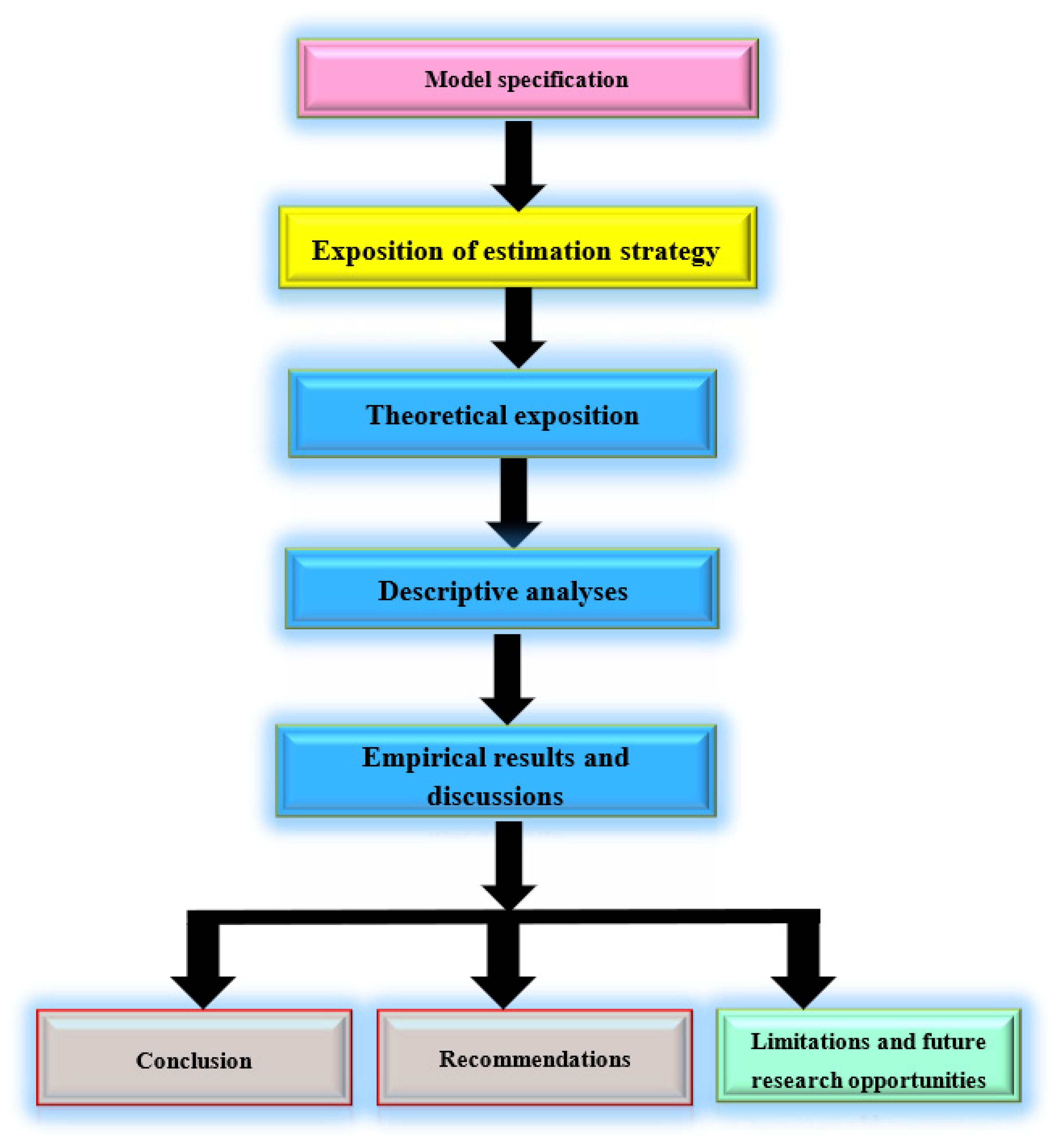
3.1. Model Specification

The empirical model of the present study is based on the highly celebrated stochastic impacts by regression on population, affluence, and technology (STIRPAT) framework proposed by [71]. Evidence abounds that the STIRPAT model is one of the most utilized and generally acceptable models in environmental research [72]. The central proposition proposed by [71] is that population and affluence would fast-track the surge in GHG emissions in the decades to come. The baseline specification of the STIRPAT model is anchored on three key factors: population (P), affluence (A), and technology (T). The equation can be stated thus:

$$I=\theta P_i^{\phi 1}\times A_i^{\phi 2}\times T_i^{\phi 3}\times {\varpi }_i$$

(1)

Giving that $\theta$ denotes the constant which scales the model. More so, the exponents of P, A, and T are represented by ${\phi }_{1\dots 3}$ in that order. The linear form of Equation (1) can be stated thus

$$\ln I_{it}={\theta }_0+{\phi }_1(\ln P_{it})+{\phi }_2(\ln A_{it})+{\phi }_2(\ln T_{it})+{\varpi }_i$$

(2)

Following the extant literature [2,4] with few amendments in line with the focus of this study, I denotes carbon emissions per capita ($co2pc$) which captures environmental quality, P denotes population growth (POPG), A is affluence represented by GDP per capita as (income) and T is technology as (TECH). The model is further expanded to capture other determinants of environmental quality, e.g., renewable energy (RE) consumption, non-renewable energy (NRE) consumption, total natural resource rents (TNRR), human capital (HC), and financial inclusion (FININCL). The set of control variables comprising foreign direct investment (FDI), trade openness (TO), and infrastructure (INFO) are equally stated. For precision purposes and to enhance the interactive terms in the models that will be estimated, we categorize the regressors into two groups. The first group comprises the principal independent variables (PIV): renewable energy, non-renewable energy, total natural resource rents, human capital, and financial inclusion. The second set comprises the control variables (CV): income, technology, foreign direct investment, trade openness, and infrastructure.

In addition, it is pertinent to note that two main models are estimated in this study according to the conditioning role of income level and technological progress. This is necessary considering the quadratic nature of the conditioning effects to be equally estimated. As such, we hold either income or technology constant depending on the model being estimated. Hence for the technology model in Equation (3), we assume income as constant, and the model is stated thus in the dynamic form:

$$\begin{array}{l}\ln co2p{c}_{it}={\theta }_0+{\phi }_1(\ln RE{C}_{it})+{\phi }_2(\ln NR{E}_{it})+{\phi }_3(\ln NTR{R}_{it})\\ +{\phi }_4(POP{G}_{it})+{\phi }_5(\ln H{C}_{it})+{\phi }_6(\ln FinInc{l}_{it})+{\phi }_7(\ln TEC{H}_{it})\\ +{\phi }_8(\ln TECH\times PI{V}_{it})+{\phi }_9(\ln FD{I}_{it})+{\phi }_{10}(\ln T{O}_{it})+{\phi }_{11}(\ln INF{R}_{it})+{\varpi }_i\end{array}$$

(3)

Equation (3) can be modified to include income while technology is held constant.

$$\begin{array}{l}\ln co2p{c}_{it}={\theta }_0+{\phi }_1(\ln RE{C}_{it})+{\phi }_2(\ln NR{E}_{it})+{\phi }_3(\ln NTR{R}_{it})\\ +{\phi }_4(POP{G}_{it})+{\phi }_5(\ln H{C}_{it})+{\phi }_6(\ln FinInc{l}_{it})+{\phi }_7(\ln incom{e}_{it})\\ +{\phi }_8(\ln income\times PI{V}_{it})+{\phi }_9(\ln FD{I}_{it})+{\phi }_{10}(\ln T{O}_{it})+{\phi }_{11}(\ln INF{R}_{it})+{\varpi }_i\end{array}$$

(4)

3.2. Estimation Technique

Estimating the relationships stated in Equations (3) and (4) is usually confronted with the issue of endogeneity which tends to restrict the reliability and validity of parameter estimates. By extension, this affects the extent to which the outcomes can be used in drawing plausible policies for addressing the pervasive issue of environmental degradation in the SSA region. The problem of endogeneity may be attributed to the probable bi-directional effects between the outcome and independent variables. For instance, increasing population rate may constitute threats to the environment by stimulating a rise in non-renewable energy consumption, food demands, and congestion of the urban area, among others. On the other end, an unhealthy environment may hinder longevity due to exposure to contagious and life-threatening diseases. Analogous cases apply to other regressors. As a result, the issue of endogenous poses significant hindrances to the clarity of the emanating impacts of the regressors on the outcome variable.

Furthermore, since the study seeks to estimate the dynamic nexuses among the variables of interest, there is a need to include the lag value of the outcome variable among the group of explanatory variables on the right-hand side. This constitutes yet another demanding challenge on the possibility of estimating the stated models. Alluding to this assertion, [73,74] advance that first-order autoregressive term (AR1) in dynamic models characterized by large N and small T is bound to face challenges emanating from unobserved country-specific variables that are inherent in the disturbance terms. In a situation of this kind, OLS and within-group estimators become inconsistent and biased, prompting the need to resort to a better and more sophisticated estimator such as the system-generalized method of moment (SYS-GMM) proposed by [75,76,77]. Five primary motivations have proved eminent in advancing the choice of the GMM estimator adopted in this study. First, when a good fit is questionable due to the persistent nature of the dependent variables, GMM becomes the most appropriate estimator. Second, in a situation where the number of countries (N) surpassed the years per country (T), GMM becomes a suitable option. Looking at the present study, it will be observed that the N(42) > T(15) thus fulfilling the essential condition for the GMM estimator. Third, the GMM estimator accounts for the potential issue of endogeneity inherent in all regressors. Fourth, the variations that are usually present in a cross-country panel model require the choice of a GMM estimator. Fifth, following the benefit and functional role of the GMM estimator, explicated in point fourth, endorsed the system GMM estimation technique [76] as a more suitable approach than the difference estimator from [75].

Consistent with the extant studies, the present study employs the [77] method, which improves [75] and considers the forward orthogonal deviations in replacement of the first differences. In particular, this extended estimator has proven to be efficient in controlling for cross-country dependence and restricting instrumental variables proliferation or limiting over-identification [32]. Further, to control for the problem of heteroscedasticity, a two-step method is employed. This is important because the one-step method is characterized by homoscedasticity.

Following the above expositions, the following equations in levels (5) and first difference (6) summarize the typical procedures for the system GMM estimation technique.

$$\ln co2p{c}_{it}={\theta }_0+{\phi }_1\ln co2p{c}_{it-\tau }+{\phi }_{2}PI{V}_{it}+{\displaystyle \sum _{h=1}^3\varphi G_{h,i,t-\tau }}+{\pi }_i+{\sigma }_t+{\varpi }_{i,t}$$

(5)

$$\begin{array}{l}\ln co2p{c}_{it}-\ln co2p{c}_{it-\tau }={\theta }_0+{\phi }_1(\ln co2p{c}_{it-\tau }-\ln co2p{c}_{it-2\tau })+{\phi }_2(PI{V}_{it}-PI{V}_{it-\tau })\\ +{\displaystyle \sum _{h=1}^3{\varphi }_h(G_{h,i,t-\tau }-G_{h,i,t-2\tau })}+({\sigma }_t-{\sigma }_{t-\tau })+{\varpi }_{i,t-\tau }\end{array}$$

(6)

The regressors are previously defined. $\tau$ denotes the coefficient of the auto-regression with a year lag assumed to be appropriate to control for past information ${\sigma }_t$ and ${\pi }_t$ represent the and country time-specific effects, respectively, while ${\varpi }_{i,t}$ indicates disturbance term.

Worthy of mentioning in the study’s model specifications are the pitfalls observed regarding the interactive regressions following [78]. The authors opine that all significant indicators in the model should be included in the specifications, and their parameters should equally be interpreted as conditional marginal effects.

3.3. Brief Expositions on System GMM Post Estimation Tests

Among the various diagnoses of the SYS-GMM estimator, both identification and exclusion restrictions are well-documented in the literature [2,32]. In effect, all regressors are taken as predetermined or assumed endogenous. Another issue of prevalence in the cross-sectional dataset is simultaneity which is resolved by employing the lagged values of the independent variables. More so, to moderate the impact of fixed effects (which has the possibility of affecting the estimated nexus), Ref. [75] suggested the use of Helmet transformations for the explanatory variables. The change entails forward mean-differencing the variables such that the average of all expected observations is deducted from the variables against subtracting the previous observations from the present ones [32]. Notwithstanding the number of lags, minimization of data loss is achieved through the computation of transformation for all observations but with the exclusion of the last from every cross-section. Moreover, Ref. [77] posits that, since the lagged observations are not employed in the formula, they become as valid as instruments.

Following the above narratives, there are possibilities that the instruments employed or years of observation considered in the panel, which are firmly assumed exogenous, may exclusively affect environmental quality through the endogenous regressors. Consequently, we evaluate the statistical significance of this exclusion and restriction via the Difference in Hansen Test (DHT) for instrument exogeneity. More importantly, the null hypothesis of DHT should not be rejected for the instruments to explain environmental quality through the endogenous regressors exclusively. However, an estimation of instrumental variable (IV) with the outcome of rejecting the null hypothesis of the Sargan Overidentifying Restrictions (OIR) test shows that such instruments are invalid and thus fail to exclusively describe the explained variable [24]. It is worth mentioning that the DHT is employed in evaluating whether years of observations employed are strictly exogenous. Conclusively, the rule of thumb regarding DHT is that failure to accept the null hypotheses of DHT corresponding to IV (year, eq (diff)) implies the validity of the exclusion restriction.

In addition to the above-explicated tests, the estimate models of GMM are usually subjected to four additional criteria. First, the second-order autocorrelation (AR (2)), which hypothesizes the non-existence of autocorrelation in the residuals, should not be rejected. Second, the null hypotheses of both the Sargan and Hansen over-identification restrictions (OIR) tests, which posit that instruments are valid or uncorrelated with disturbance terms, should not be rejected. Third, it is pertinent to state that, of the two OIR tests, more credence is given to the Hansen OIR since it is robust (though weakened by instruments) as against the Sargan OIR test, which is not robust despite being resistant to weakness by instruments. The standard practice often employed to limit the proliferation or restrict identification instruments is to ensure that the number of countries are larger than instruments in the model. Given this, the present study addresses this issue in all the estimated models. Fourth, for the overall validity of the estimated coefficient to be confirmed, the Fischer test should be significant [24,32].

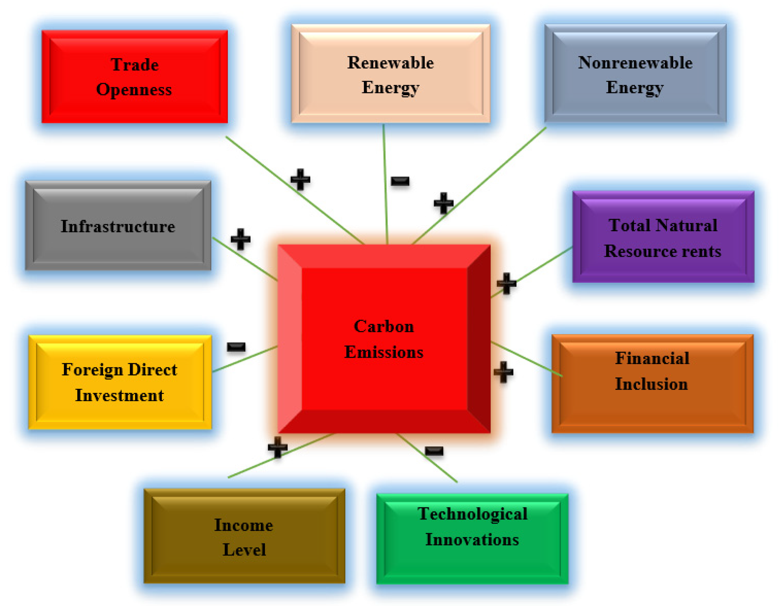
3.4. Theoretical Intuition of the a Priori Expectations

The anticipated signs of the regressors are explained in what follows. First, it should be noted that the term environmental quality is used in relative terms to denote the trend in carbon emissions per capita. Subsequently, environmental quality is said to improve when carbon emissions per capita are reducing. The reverse case explicates deterioration in environmental quality. Consequently, renewable energy is expected to improve the environment by reducing $co2p{c}_{it}$ [79]. As such, a negative sign is hypothesized so that ${\phi }_1=\left(\frac{\partial co2p{c}_{it}}{\partial REC}<0\right)$. Non-renewable energy is anticipated to deter environmental quality by enhancing the levels of $co2pc$ [2]. In effect, a positive sign is expected ${\phi }_2=\left(\frac{\partial co2pc}{\partial NRE}>0\right)$. Empirical evidence has advanced that the streams of income (rents) generated from the extraction of natural resources lead to continuous depletion of the resources irrespective of their social and environmental damages that usually occur afterward. This unchecked desire for rent increases the depletion of natural resources leading to an increase in $co2pc$ carbon emissions. As such, a positive sign is envisaged ${\phi }_3=\left(\frac{\partial co2pc}{\partial TNRR}>0\right)$. An increase in the rate of population growth is said to increase the consumption of energy, demand for food, and congestion of the urban areas. These scenarios have increasing impacts $co2pc$, translating to positive nexus between population growth (POPG) and $co2pc$ [57,58]. Hence, ${\phi }_4=\left(\frac{\partial co2pc}{\partial POPG}>0\right)$. According to available evidence in the literature, human capital (HC) can significantly reduce carbon emissions on the one hand [42] and/or increase it [14,19]. In such situations, HC can either reduce $co2pc$${\phi }_5=\left(\frac{\partial co2pc}{\partial HC}<0\right)$ or increase it ${\phi }_5=\left(\frac{\partial co2pc}{\partial HC}>0\right)$.

The role of financial inclusion has equally been argued from two angles. Some scholars believe that financial inclusion increases the stock of carbon emissions [11], while some hold the view that it reduces carbon emissions [70]. Consequent upon these diverging views, we anticipate positive sign ${\phi }_6=\left(\frac{\partial co2pc}{\partial FinIncl}>0\right)$ or negative sign ${\phi }_6=\left(\frac{\partial co2pc}{\partial FinIncl}<0\right)$s. The impact of technology on carbon emissions is expected to be negative [2,80]. By implication, the negative sign is hypothesized ${\phi }_7=\left(\frac{\partial co2pc}{\partial TECH}<0\right)$. Further, the impacts of income have been accorded valuable attention in the environmental debates, especially with views that it retards quality environment by enhancing increase in carbon emissions of nations in the early stage of economic development [24]. Contrarily, an increase in income level to a certain threshold will promote the preference for consumption of environmental-friendly goods, demand for cleaner energy, and drive toward green growth. Consequently, positive ${\phi }_6=\left(\frac{\partial co2pc}{\partial incomel}>0\right)$ or negative signs ${\phi }_6=\left(\frac{\partial co2pc}{\partial income}<0\right)$ are hypothesized.

Notwithstanding the foregoing, the a priori expectations of the conditioning roles of income and technology take a different dimension. The reason being that, in Equations (3) and (4), the parameters that are required in analysing the impacts of PIV on environmental quality in the presence of technological advancement and income level are ${\phi }_{1\dots 6}$ and ${\phi }_8$. It is pertinent to observe that the presence of the interaction in the aforementioned equations alters how the impacts of PIV on environmental quality are interpreted. For this reason, an increase in PIV will enhance (deter) environmental quality subject to improvement (disimprovement) in either of technological progress or income [81]. Since ${\phi }_8$ denotes the interactive impacts of PIV and the conditioning variables (technology and income), a statistically significant and positive value will imply that advancement in technology (or increase in income) complements PIV to improve (deter) environmental quality. It is worthy of explaining that parameters ${\phi }_{1\dots 6}$ capture the impacts of PIV on environmental quality (co2pc) as the conditioning variables improve by partial derivative of co2pc.

$$\frac{\partial co2p{c}_{it}}{\partial PI{V}_{it}}={\phi }_{1\dots 6}+{\sigma }_{8}TEC{H}_{it}$$

(7)

$$\frac{\partial co2p{c}_{it}}{\partial PI{V}_{it}}={\phi }_{1\dots 6}+{\sigma }_{8}incom{e}_{it}co2pc$$

(8)

3.5. Data, Descriptive and Contextual Analyses

The empirical analyses in this study are based on panel data collected from the World Development Indicators from 2004 to 2018. The choice of start period is influenced by the availability of data on most of the critical variables from 2004 (especially financial inclusion). The end period (2018) is equally chosen because succeeding years do not contain the dataset for most of the variables.

From the descriptive statistics (

Table 1. Descriptive statistics.

Variables	Name and Measurements	Mean	Std. Dev.	Maximum	Minimum	Signs
CO2	CO2 emissions (metric tons per capita)	1.54231	2.544378	9.979458	0.02801	Nil
REC	Renewable energy consumption (% of total final energy consumption)	31.08094	29.71533	97.01889	0.354019	−ve
NRE	Non-renewable energy (Fossil fuel energy consumption % of total)	61.16206	28.50543	88.14867	0	+ve
TNRR	Total natural resource rents (% of GDP)	12.10421	12.68515	59.20581	0.001259	±ve
FININCL	Financial inclusion (automated teller machines (ATMs) per 100,000 adults)	13.12443	16.12839	65.69298	0.019368	±ve
POPG	Population growth (annual %)	2.253501	1.01767	3.907245	−0.61666	+ve
HC	Human capital (school enrollment, primary % gross)	104.2626	13.13886	139.9336	62.70836	±ve
TECH	Technology (ICT service exports % of service exports, BoP)	6.243425	6.815692	52.30411	0.338888	−ve
INCOME	GDP per capita (constant 2010 US$)	2877.072	2811.481	11124.66	215.1546	±ve
FDI	Foreign direct investment, net inflows (% of GDP)	4.616172	5.887718	39.4562	−3.85111	±ve
INFR	Fixed telephone subscriptions (per 100 people	5.168841	8.127514	31.06683	0	−ve
TO	Trade-in services (% of GDP)	18.66079	13.56806	70.23726	4.699146	±ve

), it is apparent that the mean value of carbon emissions per capita for the study period is 1.54. This average value accentuates the view held in the literature that Africa contributes less to global GHG emissions [2]. That notwithstanding, evidence still projects the continent as the most vulnerable to global GHG emissions in the future [82]. Moreover, several internal factors contribute to the persistent rise in SSA’s carbon emissions, of which land degradation stands out. Available statistics show that land degradation constitutes a substantial environmental problem combating the wellbeing of the population in the region. According to [30], a special report by IPCC submits that 46% of the landmass in Africa is susceptible to degradation, which has affected not less than 485 million of the population and leading to estimated annual costs of $9.3 billion. Regarding the mean values of energy consumption, it is apparent that NRE consumption (61.16) surpasses REC consumption (31.08) which suggests that the SSA is still reliant on traditional energy [2,79].

The average value of total natural resource rents (TNRR) of 12.10 is below the annual record of 20.04 in 2008. Historically, TNRR has maintained a fluctuating trend in the last two decades due to the instability in the global oil price. Going by WDI records, between 2004 and 2008, TNRR records a persistent increase; however, following the global financial crisis in 2008, which had its multiplier effects on other sectors of the global economy, declining trends were evident from 2009 to 2010 with a slight increase in 2011. This did not last long as a sharp decline was recorded in 2012 through 2016, which are the years of intense worldwide drop in oil prices. Worrisome enough, the diminishing level of TNRR has refused to improve until the present moment. That notwithstanding, whether the environmental impacts of this indicator will decline is hard to tell.

The mean value of financial inclusion in SSA stands at 13.12 for the period under study. Generally, the region is recording a considerable number of the unbanked population despite the recent progress being recorded in the banking industry. As of 2014, nearly 350 million people are financially excluded in SSA, with significant issues hinging on a persistent increase in poverty and restricted physical banking infrastructure [24]. Though, recent strides in SSA concerning digitalization are helping to close the gaps, reports still hold that many people are financially excluded in the region [80]. When people are financially excluded, they lack the financial capacity to access environmentally friendly goods and services. With their low economic status coupled with the desire to meet their basic needs, they are forced to consume more of emission-embedded products, which subsequently deter the environment.

Population growth which averages 2.3 further corroborates the recent rate of 2.7 for the region. Population growth is one of the most often cited factors militating against attaining sustainable environment (SDG 2) in SSA [83]. Ref. [28] report submits that population growth in SSA will witness a rise from 1.07 billion in 2019 to a record high of 3.78 billion come 2020. The devastating ecological threat of the anticipated population explosion could become unbearable if drastic actions are not taken today in the interest of future generations. The average value of human capital, which stands at 104.3, implies an improvement in the region’s human development at the primary level of education. Generally, enrolment at the primary school level is usually the highest for the SSA in the last three decades or more [84]. This suggests that more people are educationally inclusive at the lower level in the region. The average value of technology which is 6.24, further confirms that technology advancement is still at the early stage in SSA [2]. The income level in the region, which averages 2877.1, suggests the region is doing well economically. Available statistics show that the SSA region is doing great on the GDP performance metrics in the last two decades, with an approximately 60% rise [85]. In addition to the South Asia region, development metrics in SSA constitute the fastest growing among emerging regions of the world [86].

4. Empirical Results and Discussion

The estimated results are presented and discussed in this section. Notably, the models are presented in two categories which are the technology model and income level model.

4.1. Technological Enhanced Model

The results of the estimated models illustrating the functional relationship between energy consumption, total natural resource rents, population growth, human capital, and financial inclusion on the environmental quality of the SSA region are presented in

Table 2. System GMM results on the conditioning role of technology advancement.

Variables	Independent Variable: Carbon Emissions per Capita (co2pc)
	Model 1	Model 2	Model 3	Model 4	Model 5	Model 6
L.co2	0.7268 ***	0.9287 ***	0.7835 ***	0.8969 ***	0.7671 ***	0.7736 ***
	(0.009)	(0.0034)	(0.0039)	(0.0027)	(0.0069)	(0.0029)
rec	−0.0056 ***
	(0.0012)
nre		0.0031 ***
		(0.0003)
tnrr			0.0064 ***
			(0.0016)
popg				0.2059 ***
				(0.0071)
hc					0.0033 *
					(0.0017)
finincl						0.0003
						(0.0003)
tech	−0.0257 ***	−0.0022 **	−0.0073 ***	−0.0122 ***	−0.0252 ***	−0.0022 ***
	(0.0047)	(0.0009)	(0.0021)	(0.0018)	(0.0084)	(0.0002)
tech*PIV	−0.0003 ***	0.0022	−0.0005 ***	−0.0049 ***	0.0003 ***	0.0011 ***
	(0.0001)	(0.00034)	(0.0001)	(0.0008)	(0.0001)	(0.0001)
Net effects	−0.0128	na	0.0004	0.1949	0.0279	na
to	0.0053 ***	0.0024 ***	0.0028 ***	0.0083 ***	−0.0026 **	0.0039 ***
	(0.001)	(0.0008)	(0.0004)	(0.0007)	(0.001)	(0.0005)
fdi	−0.001 **	0.0006	−0.0027 ***	−0.0008 *	−0.0026 ***	−0.0008 **
	(0.0004)	(0.0005)	(0.0003)	(0.0004)	(0.0004)	(0.0003)
infr	0.0779 ***	0.0036	0.0671 ***	0.0112 ***	0.0637 ***	0.0564 ***
	(0.007)	(0.0025)	(0.0034)	(0.0028)	(0.0048)	(0.0017)
_cons	−0.4736 ***	−0.0488 **	−0.147 ***	−0.5894 ***	0.3015	−0.0877 ***
	(0.1011)	(0.0187)	(0.0302)	(0.0144)	(0.1913)	(0.0142)
AR1	0.227	0.027	0.212	0.168	0.266	0.213
AR2	0.289	0.210	0.277	0.223	0.316	0.274
Sargan OIR	0.000	0.000	0.000	0.000	0.000	0.000
Hansen OIR	0.229	0.580	0.162	0.177	0.114	0.410
DHT for instruments (a) Instruments in levels
H excluding group	0.317	0.213	0.026	0.108	0.199	0.104
Dif(null, H = exogenous	0.246	0.821	0.695	0.394	0.162	0.796
(b) IV (years, eq(diff))
H excluding group	0.192	0.521	0.1840.	0.162	0.098	0.360
Dif(null, H = exogenous	0.753	0.000	0.179	0.411	0.499	0.752
Fisher	63.86 ***	84.58 ***	10.90 ***	19.59 ***	80.46 ***	17.67 ***
Instruments	32	32	32	32	32	32
Country	42	42	42	42	42	42
Observations	391	219	426	426	359	344

***, **, * denotes significance levels at 1%, 5% and 10% in that order. The term tech*PIV implies the multiplicative effects of technology and each variable of the principal independent variables. Dif stands for Difference. OIR denotes Over-identifying Restrictions Test. DHT means Difference in Hansen Test. The bolded values denote two levels of significance thus. First refers to the statistical significance level of the Fisher test and the coefficients estimated. The second implies acceptance of the null hypotheses of no autocorrelation in the AR(1) and AR(2) tests and failure to reject the null hypotheses of the validity of the instruments in the Sargan OIR test.

and

Table 3. System GMM results on the conditioning role of income level.

Variables	Independent Variable: Carbon Emissions (co2pc)
	Model 1	Model 2	Model 3	Model 4	Model 5	Model 6
L.co2	0.7956 ***	0.8699 ***	0.7384 ***	0.6845 ***	0.7614 ***	0.7545 ***
	(0.0026)	(0.0348)	(0.0159)	(0.018)	(0.0101)	(0.0187)
rec	−0.0201 ***
	(0.0017)
nre		0.0043 ***
		(0.0017)
tnrr			0.0226 *
			(0.0131)
popg				1.3609 ***
				(0.4747)
hc					0.0095
					(0.0157)
finincl						0.0991
						(0.1219)
lnincome	0.3112 ***	0.2032 ***	0.1482 ***	0.6199 ***	0.3299	0.5093 ***
	(0.0179)	(0.0593)	(0.0404)	(0.2016)	(0.265)	(0.1114)
Income*IV	−0.0029 ***	0.0002	−0.003 *	−0.1607 **	−0.0018	0.0103 ***
	(0.0003)	(0.0002)	(0.0017)	(0.0611)	(0.0026)	(0.0023)
Net effects	−0.0382	na	0.0088	−1.6379	na	na
to	0.0018 ***	0.0017	0.0034 **	0.0083 ***	0.0007	0.0019 *
	(0.0003)	(0.0031)	(0.0015)	(0.0025)	(0.0008)	(0.0011)
fdi	−0.0005 ***	−0.0004	0.0003	−0.0011	−0.0015	−0.0029 ***
	(0.0001)	(0.0018)	(0.0004)	(0.0008)	(0.0015)	(0.0007)
infr	0.012 ***	0.0319 ***	0.0718 ***	0.1057 ***	0.0525 ***	0.0066
	(0.0036)	(0.0114)	(0.0117)	(0.0162)	(0.0072)	(0.0172)
_cons	−2.0475 ***	−1.2753 ***	−0.9668 ***	−4.8286 ***	−1.9069	−3.2581 ***
	(0.1037)	(0.3956)	(0.3024)	(1.5293)	(1.6038)	(0.7285)
AR1	0.213	0.026	0.214	0.242	0.261	0.201
AR2	0.270	0.245	0.278	0.289	0.308	0.257
Sargan OIR	0.000	0.000	0.000	0.003	0.000	0.000
Hansen OIR	0.265	0.607	0.156	0.603	0.744	0.382
DHT for instruments (a) Instruments in levels
H excluding group	0.093	0.384	0.261	0.690	0.649	0.154
Dif(null, H = exogenous	0.605	0.657	0.177	0.453	0.653	0.620
(b) IV (years, eq(diff))
H excluding group	0.251	0.384	0.139	0.535	0.768	0.332
Dif(null, H = exogenous	0.381	0.987	0.404	0.796	0.271	0.601
Fisher	67.62 ***	26.06 ***	17.93 ***	95.08 ***	12.03 ***	22.13 ***
Instruments	32	24	24	24	24	24
Countries	42	42	42	42	42	42
Observations	431	237	471	471	394	381

***, **, * denotes significance levels at 1%, 5% and 10% in that order. The term income*PIV implies the multiplicative effects of income level and each variable of the principal independent variables. Dif stands for Difference. OIR denotes Over-identifying Restrictions Test. DHT means Difference in Hansen Test. The bolded values denote two levels of significance thus. First refers to a statistical significance level of the Fisher test and the coefficients estimated. The second implies acceptance of the null hypotheses of no autocorrelation in the AR(1) and AR(2) tests and failure to reject the null hypotheses of the validity of the instruments in the Sargan OIR test.

. Specifically, Table 2 considers the nexus as mentioned earlier with the conditioning role of technology, while Table 3 considers the role of income level. In each of the tables, six models are detailing on the individual impact of the selected principal variables on the outcome variable as thus; Model 1 (renewable energy consumption (rec)), Model 2 (non-renewable energy (nre)), Model 3 (total resource rents (tnrr)), Model 4 (population growth (popg)), Model 5 (human capital (hc)) and Model 6 (financial inclusion (finincl)). Moreover, the interactive impacts of technology (tech) with each of the principal independent variables (PIV) are denoted by the product of both as (tech*PIV).

As indicated in Table 2, renewable energy consumption (rec) negatively and statistically impacts carbon emissions per capita (co2pc). This implies that renewable energy consumption has mitigating effects on co2pc in such a way that a percentage increase in renewable energy leads to a significant reduction in the stock of co2pc. Particularly, renewable energy is noted to be highly effective for achieving sustainable development [4] through the mitigation of climate change impacts [87]. This result is intuitively plausible because renewable energy is a clean class of energy sources and supports green growth. This result is consistent with extant studies that advance renewable energy’s abating role on carbon emissions [40,41]. Overall, since the African continent is richly blessed in abundance of renewable energy, tapping efficiently into it may imply an effective way of significantly minimizing the devastating effects of carbon emissions on the region’s ecosystem and longevity of the populace.

The impact of non-renewable energy (nre) is positive and statistically significant, implying that the former enhances the latter. By implication, a proportionate increase in non-renewable energy consumption leads to a substantial increase in the stock of co2pc. The SSA region in the present moment relies more on non-renewable energy for the majority of the production activities, which may suggest why the region is still finding it difficult to get out the long-embattled environmental degradation. The emanating effects of non-renewable energy on co2pc in this study confirm with previous empirical submissions in a similar view [63]. The impacts of total natural resource rents (TNRR) are positively significant in contributing to the increase in co2pc in SSA. This suggests that TNRR constitutes one of the important drivers of co2pc in the region. This sounds logical because the bulk of the revenue earnings most economies in SSA come from natural resources and other primary commodities. It is equally instructive to note that since SSA is in the group of regions with low-income countries, the drive to earn more revenues through resource rents will most likely overshadow the environmental interest. Hence, the more desire for resource rents, the more natural resources are depleted and the higher the stocks of carbon emissions. This result is inconsonant with [5,50], which hold the view that natural resource rents significantly contribute to the rise in carbon emissions.

The environmental impacts of population growth as evident in the results are statistically positive. Intuitively, a percentage increase in population growth rates lead to a corresponding increase in co2pc. The environmental impacts of population growth rates are evident from different channels, such as an increase in demand for food, of which SSA remains one of the regions facing severe food insecurity [88]. An increasing population mounts pressure on the agriculture sector to increase its production and cultivation processes to meet the excess food demand. Since the sector relies more on traditional production systems and non-renewable energy, carbon emissions will increase. The positive impacts of population growth on carbon emissions as evident in this study are consistent with extant studies [57,58]. The environmental impact of human capital is noted to be positive and statistically significant in promoting co2pc. This is plausible as awareness of the people through education may avail them the technical capacity to operate energy-intensive gadgets, which correspondingly escalate the urge in co2pc. This result agrees well with previous studies that hold that human capital promotes carbon emissions and hinders environmental quality [14,19]. Financial inclusion exerts positive but statistically insignificant effects on co2pc. This implies that, in the present moment, the level of financial inclusiveness in the SSA region is not strong enough to drive environmental quality.

The impacts of technological progress are negative and statistically significant across the models. By implication, technology has abating impacts on carbon emissions in the region. This study’s empirical result, which holds that technology reduces carbon emissions, is consistent with extant studies [2,7,63]. The interactive impacts of technology with the principal independent variables turn out to be negative. This suggests that advancements in technology enhances the abating effects of renewable energy on co2pc and reduces the inducing impacts of non-renewable energy, total natural resource rents, and population growth rates on co2pc. These results are in agreement with the mediating effects of technology reported by [2] for the G-7 economies, [2] for the G-20 countries, and [5] for the SSA region.

The results of the interactive (otherwise called marginal or conditional) effects of technology and PIV estimated in Table 2 require an assessment of the actual effects. While the emanating effects across the models are adverse, care must be taken in solemnly relying on these effects for policy implications. Hence, the standard practice in recent empirical studies has been to further compute net effects that provide the estimated model’s actual overall impacts [24,32]. According to [24], the following model is employed to estimate the net effects.

$$NE=\left(\left[MGE\times MV\right]+\left[UnE\right]\right)$$

(9)

$NE$ net effects, $MGE$ marginal (unconditional or interactive) effect, $MV$ mean value, and $UnE$ unconditional (direct) effect. Following Equation (8), the net effects in Table 2 can be computed thus.

Column 1 (REC): ([−0.0003 × 61.16] + [−0.0056]) equal −0.0239. This implies that interaction of technological progress and renewable energy is persistent in subduing carbon emissions. This is called the synergy effect [89].

Column 3 (TNRR): ([−0.0005 × 12.10] + [0.0064]) equal 0.0004. This implies that the moderating impact of the estimated interaction between technological progress and total resource rents is inconsistent. By implication, the result further implies a limit to the extent to which technology can subdue the negative effects of total resource rents on the environment. Alternatively, this can be tagged asynergy effect.

Column 4 (POPG): ([−0.0122 × 2.25] + [0.2059]) equal 0.1949. This denotes that the moderating effect of the estimated interactive term of technological progress and population growth differs from the net effect and is thus inconsistent. By implication, the result further implies a limit on the extent to which technology can subdue the negative effects of population growth on the environment.

Column 5 (HC): ([−0.0003 × 104.26] + [−0.0033]) equal 0.0004. By implication, the estimated interactive terms of technological progress and human capital is supported and persistent. In order words, the synergy effect is evident.

4.2. Income Level Enhanced Model

The structure of the empirical modelling in Table 3 (conditioning effects of income level) is similar to what is obtainable in Table 2 (conditioning effects of technological progress) above. Hence, the mainline of difference is just the replacement of technology with income level. As such, Table 3 presents the empirical results on the impacts of PIV, income, and the interaction of both on environmental quality captured by co2pc in SSA.

Taking a close look at the table, it will be evident that the emanating results are robust for Table 2. This is particularly obvious for indicators such as renewable energy, non-renewable energy, total natural resource rents, and population growth rates. Moreover, the impacts of income across the model are positive and statistically significant. This implies that the income level of the economies in SSA is not high enough to promote green growth and the environment. Following the EKC propositions, nations at the lower-income level tend to experience significant degradation due to heavy reliance on traditional energy sources and high poverty rates. Environmental regulations are usually relaxed for the importation of dirt goods in a bit to complement local shortage. The interaction of income with PIV shows some level of divergences in their effects. For instance, renewable energy-income interaction exerts a negative impact on co2pc, which implies that irrespective of access to income at any level, carbon abating impact of renewable energy is persistent. More so, the outcomes of the interaction of other explanatory variables, such as total natural resource rents and population growth on carbon emissions, are significant. This implies that a corresponding increase in income and TNRR may stimulate a substantial reduction in environmental pollution. This is achievable with proper investments of the income earned from natural resource rents and the economy’s overall income in clean energy resources.

The interaction of population growth with income produces moderating effects on carbon emissions. The plausibility of these results lies in the fact that an increase in income would afford household consumers adequate access to good health care services and spend more on environmentally friendly goods and services. The interaction of income and financial inclusion turns out to be positive, implying access to income increases access to financial services and subsequently avails the household consumption of the financial capability to acquire energy-intensive products. Moreover, with more income, demand for goods and services will increase, increasing the production process in traditional energy and environmental pollutant economic activities. Since the computation of net effects as previously discussed, we will only focus on the emerging overall impacts. For instance, in Model 1 (REC-income nexus) and Model 3 (TNRR-income nexus), synergy effects are evident, while the asynergy effect is supported in Model 4 (Population growth-income nexus).

Overall, the analyses presented in Table 3 show that income level is insufficient to lessen carbon emissions per capita, though the interplay of other vital variables could still prove efficient.

The respective impacts of the control variables are explained thus. Trade openness contributes positively to carbon emissions across most of the models where it is significant. This implies trade openness contributes to the surge in environmental pollution of the SSA countries. This result is intuitional for the SSA region, which mainly comprises low and middle-level income economies. This result is consistent with previous studies which hold that trade openness promotes carbon emissions in lower and middle-income countries [7,15]. The theoretical justification for this outcome could be based on the pollution haven hypothesis, which postulates the settlement of pollution-intensive sectors from developed economies to their emerging counterparts, thus leading to the transfer of pollution from the former to the latter. Positive effects are equally evident in the impacts of infrastructure across the significant models. This implies that an increase in infrastructure facilities leads to a corresponding rise in co2pc. This could be because an increase in social amenities could trigger the consumption of energy-intensive products and services. Since the SSA region relies more on traditional energy, which is carbon-intensive, the environment becomes more polluted.

Adverse effects are evident across the significant models in the relationship between foreign direct investment (FDI) and carbon emissions. This implies that FDI promotes a quality environment by mitigating the surge in carbon emissions. The enhancing role of FDI on the quality environment is anchored on the ground that FDI promotes cleaner and greener technologies in host economies [90]. Moreover, empirical evidence has established that multinational corporations are usually more environmentally conscious in host countries by adopting efficient management practices and environmentally friendly technology [91].

The post estimation tests of validity for the Sys-GMM estimates fulfill all stated criteria. For instance, the Arellano-Bond statistics, AR (1), and AR (2) test hypothesizing the case of no first and second-order residual serial correlations are not rejected. Moreso, while we fail to accept the null hypothesis of the Sargan OIR tests, we fail to reject the Hansen OIR tests of instrument validity. Moreover, the validity of the overall models is confirmed by the significant levels of Fisher across all the models. Further, the persistence criterion requiring positive significance and within zero less range for the lag values of the dependent variables is fully achieved. A graphical representation of the findings is presented in Figure 2.

4.3. Robustness Check: Extensions for Other Levels of Carbon Emissions

The empirical results in Table 2 and Table 3 have established reasonable evidence on the functional nexus between PIV and environmental quality in SSA with the conditioning roles of technological progress and income level. That notwithstanding, we embark on a robustness check to help widen our understanding of the relationships being assessed. According to [92], a robustness check is an empirical analysis conducted to appraise how regression coefficient estimates will react due to alterations in the model by adding or removing key variables. Consequent upon that, we consider four different classes of carbon emissions with the following indicators; carbon emission measured in kiloton (co2kt), agricultural methane emissions measured in thousand metric tons of CO₂ equivalent (co2agr), CO₂ emissions from residential buildings, and commercial and public services measured as % of total fuel combustion (co2res), and CO₂ emissions from transport measured as % of total fuel combustion (co2trans). Two tables are presented on the results of this section for technological advancement and income level. Two models are estimated for each of the new outcome variables. Model 1 examines the underlining relationship with the inclusion of technology while Model 1 excludes technology.

Going by the results in

Table 4. System GMM results on the PIV-environmental quality nexus (with and without technological advancement).

	rec-lnco2kt		nre-lnco2kt		rec- co2res		nre- co2res		rec-co2trans		nre-co2trans		rec- co2agr		nre- co2agr
	Model 1	Model 2	Model 1	Model 2	Model 1	Model 2	Model 1	Model 2	Model 1	Model 2	Model 1	Model 2	Model 1	Model 2	Model 1	Model 2
L.lnco2kt	0.803 ***	1.016 ***	0.866 ***	0.89 ***	0.951 ***	0.936 ***	0.911 ***	0.922 ***	0.722 ***	0.744 ***	0.723 ***	0.817 ***	0.722 ***	0.724 ***	0.831 ***	0.909 ***
	(0.054)	(0.029)	(0.038)	(0.017)	(0.034)	(0.056)	(0.045)	(0.033)	(0.039)	(0.033)	(0.081)	(0.044)	(0.039)	(0.041)	(0.036)	(0.042)
rec	−0.009 ***	−0.005 **			0.026	−0.013			−0.077	−0.075			69.685 ***	18.461
	(0.002)	(0.002)			(0.032)	(0.017)			(0.106)	(0.044)			(21.348)	(24.895)
nre			0.005 ***	0.008 ***			0.045 *	0.003			0.077 *	0.032 *			5.773 ***	2.784 **
			(0.001)	(0.002)			(0.022)	(0.012)			(0.032)	(0.016)			(1.657)	(0.632)
tnrr	0.017 ***	0.002	0.009 ***	0.001	0.064 ***	0.005	0.058 ***	0.014	0.085	−0.127	0.140	−0.067	0.1210.363 *	−30.21	43.226	11.276
	(0.004)	(0.003)	(0.002)	(0.003)	(0.015)	(0.018)	(0.015)	(0.017)	(0.052)	(0.082)	(0.134)	(0.088)	(58.7)	(56.496)	(49.307)	(111.369)
hc	0.011 **	0.005 **	−0.003	0.001	0.053 ***	0.085 ***	0.036 **	0.075 ***	0.344 **	0.174 **	0.16	0.107	93.807 *	54.26 **	95.713	−11.276
	(0.004)	(0.002)	(0.002)	(0.001)	(0.018)	(0.010)	(0.012)	(0.011)	(0.158)	(0.07)	(0.12)	(0.082)	(53.767)	(24.753)	(97.489)	(50.608)
popg	0.097 ***	0.012 **	0.153 ***	0.017	0.802	0.335	0.681 ***	0.368 ***	4.395 **	3.181 **	2.714 ***	1.777 ***	1893.53	1036.001 *	20.603 ***	89.243 ***
	(0.017)	(0.004)	(0.052)	(0.053)	(0.831)	(0.289)	(0.064)	(0.072)	(1.855)	(1.188)	(0.9)	(0.234)	(1182.107)	(590.179)	(1.421)	(9.768)
finincl	0.005 **	0.011 ***	0.001	0.003	0.012	0.017	0.016	0.023 **	0.018	0.182 ***	0.023	−0.014	−19.216	−34.072	−42.334	−43.635
	(0.002)	(0.001)	(0.002)	(0.002)	(0.009)	(0.016)	(0.012)	(0.01)	(0.03)	(0.045)	(0.032)	(0.05)	(49.485)	(42.514)	(117.671)	(77.465)
tech	−0.01 ***		−0.014 ***		−0.035 **		−0.003		−0.095 *		0.082		−39.549		−214.513 **
	(0.002)		(0.003)		(0.017)		(0.002)		(0.048)		(0.053)		(104.309)		(86.161)
to	−0.016 ***	−0.005 **	−0.009 ***	−0.006 **	−0.067 **	−0.015	−0.069 **	0.028	0.053	−0.055	0.148	−0.025	−19.249	−56.137 **	−20.73	−11.626
	(0.003)	(0.002)	(0.003)	(0.003)	(0.029)	(0.03)	(0.042)	(0.025)	(0.07)	(0.083)	(0.17)	(0.043)	(46.588)	(21.163)	(32.158)	(49.771)
fdi	0.001	0.002	−0.004	0.001	−0.101 **	−0.039 *	−0.099 **	−0.061 **	−0.17 *	−0.123 **	−0.021	−0.027	65.047	76.297	28.208	−0.062
	(0.001)	(0.004)	(0.003)	(0.003)	(0.021)	(0.02)	(0.039)	(0.022)	(0.087)	(0.05)	(0.111)	(0.032)	(211.573)	(56.92)	(144.899)	(124.828)
_cons	3.814 ***	0.725 *	1.423 ***	0.797 ***	−0.248 **	−0.753 **	−2.893	−0.914 **	−30.381	−4.992	−12.857	−3.67	7027.816	6026.432 *	−10,606.406	1037.686
	(0.865)	(0.416)	(0.422)	(0.23)	(0.063)	(0.204)	(2.949)	(0.312)	(19.373)	(8.944)	(18.521)	(8.844)	(8380.527)	(3019.672)	(13,117.383)	(7353.675)
AR1	0.033	0.012	0.168	0.020	0.125	0.107	0.130	0.110	0.167	0.159	0.089	0.063	0.071	0.090	0.000	0.026
AR2	0.599	0.711	0.314	0.500	0.483	0.414	0.468	0.458	0.582	0.412	0.216	0.131	0.706	0.837	0.453	0.465
Sargan OIR	0.000	0.000	0.000	0.000	0.673	0.523	0.690	0.499	0.000	0.000	0.001	0.000	0.865	0.374	0.766	0.660
Hansen OIR	0.623	0.231	0.631	0.639	0.987	0.972	0.990	0.929	0.971	0.999	0.978	0.957	0.750	0.799	0.899	0.991
DHT for instruments (a) Instruments in levels
H excluding group	0.687	0.388	0.910	0.425	0.774	0.950	0.428	0.865	0.577	0.722	0.447	0.467	0.429	0.731	0.931	0.761
Dif(null, H = exogenous	0.482	0.208	0.348	0.682	0.982	0.870	0.872	0.819	0.986	0.896	0.998	0.991	0.789	0.548	0.999	0.989
(b) IV (years, eq(diff))
H excluding group	0.584	0.190	0.570	0.480	0.980	0.960	0.984	0.904	0.974	0.964	0.892	0.941	0.832	0.521	0.999	0.924
Dif(null, H = exogenous	0.556	0.826	0.987	0.988	0.873	0.865	0.866	0.764	0.334	0.989	0.667	0.876	0.137	0.956	0.844	0.675
Fisher	91.44 ***	13.84 ***	58.69 ***	30.31 ***	19.85 ***	11.08 ****	23.49 ***	13.65 ***	49.81 ***	84.95 ***	11.17 ***	90.28 ***	63.45 ***	28.49 ***	65.37 ***	48.95 ***
Instruments	32	32	32	32	32	32	32	32	32	32	32	32	32	32	32	3
Countries	42	42	42	42	42	42	42	42	42	42	42	42	42	42	42	42
Observations	264	290	149	159	136	146	135	145	142	152	134	144	79	90	54	59

***, **, * denotes significance levels at 1%, 5% and 10% in that order. The term income*PIV implies the multiplicative effects of income level and each variable of the principal independent variables. Dif stands for Difference. OIR denotes Over-identifying Restrictions Test. DHT means Difference in Hansen Test. The bolded values denote two levels of significance thus. First refers to the statistical significance level of the Fisher test and the coefficients estimated. The second implies acceptance of the null hypotheses of no autocorrelation in the AR(1) and AR(2) tests and failure to reject the null hypotheses of the validity of the instruments in the Sargan OIR test.

, the impacts of renewable energy consumption (rec) are negative and statistically significant for two variants of carbon emissions which are co2kt and co2agr. In the former, the moderating effects of renewable energy are substantial both in the model with and without technology. This suggests that technology can only further enhance renewable energy in checkmating the rising level of carbon emissions, but its absence would not undermine the negative connection. In the co2agr model, renewable energy only reduces carbon emissions from the agriculture sector when technology is in the model. Hence, renewable energy is far from lessening carbon emissions produced in the agricultural sector without employing technology in farming and other agricultural practices. Non-renewable energy (nre) promotes all four sets of carbon emissions with and without the interplay of technology.

Further, other indicators in the group of PIV which contribute to the surge in carbon emissions include human capital, population growth, and financial inclusion. This contributive role is evident with and without technology. In order words, it could be inferred that the level of technological advancement in the SSA is still not sophisticated enough to suppress the contributions of some pollutants drivers in promoting carbon emissions. The adverse nexus between technology and carbon emissions are empirically supported in all the estimated models, especially those with statistical significance. Summarily, the empirical results from Table 4 based on the technology model show that the previous results in Table 2 are robust and empirically supported to explain variations in the level of carbon emissions in SSA.

The empirical outcomes in

Table 5. System GMM results on the PIV-environmental quality nexus (with and without income level).

	rec-lnco2kt		nre-lnco2kt		rec-co2res		nre-co2res		rec-co2trans		nre-co2trans		rec-co2agr		nre-co2agr
	Model 1	Model 2	Model 1	Model 2	Model 1	Model 2	Model 1	Model 2	Model 1	Model 2	Model 1	Model 2	Model 1	Model 2	Model 1	Model 2
L.lnco2kt	0.831 ***	0.99 ***	0.765 ***	0.857 ***	0.724 ***	0.862 ***	0.741 ***	0.887 ***	0.491 ***	0.744 ***	0.817 ***	0.817 ***	0.857 ***	0.831 ***	0.929 ***	0.926 ***
	(0.037)	(0.025)	(0.036)	(0.035)	(0.046)	(0.046)	(0.05)	(0.04)	(0.033)	(0.033)	(0.044)	(0.044)	(0.038)	(0.036)	(0.041)	(0.036)
rec	−0.006 ***	−0.002			−0.066 **	−0.020			−0.308 ***	−0.075			0.526	18.461
	(0.002)	(0.002)			(0.026)	(0.019)			(0.074)	(0.044)			(26.187)	(24.895)
nre			0.008 ***	0.007 ***			0.096 ***	0.002			0.032 ***	0.032			1.838 **	2.784 **
			(0.002)	(0.001)			(0.031)	(0.018)			(0.006)	(0.036)			(0.988)	(0.632)
tnrr	0.001	0.003	0.003	0.005 ***	0.06 ***	0.033	0.073 ***	0.025 **	0.134	−0.127	−0.067	−0.067	9.366	−30.21	8.65	11.276
	(0.003)	(0.002)	(0.003)	(0.002)	(0.018)	(0.020)	(0.021)	(0.01)	(0.124)	(0.082)	(0.088)	(0.088)	(62.519)	(56.496)	(113.32)	(111.369)
hc	0.002 *	0.007 ***	0.005	0.003 **	0.029	0.058 **	0.033	0.046	0.195 *	0.174 **	0.107	0.107	45.511 *	54.26 **	−7.603	−11.276
	(0.001)	(0.002)	(0.003)	(0.001)	(0.028)	(0.025)	(0.026)	(0.028)	(0.1)	(0.07)	(0.082)	(0.082)	(25.061)	(24.753)	(51.385)	(50.608)
popg	0.023 ***	0.024 ***	0.131 *	0.186 ***	1.003 ***	1.039 **	0.227 ***	2.208 ***	2.534 ***	3.181 **	1.777 ***	1.977 ***	658.41	1036.001 *	922.062 ***	892.427 ***
	(0.003)	(0.008)	(0.069)	(0.053)	(0.715)	(0.582)	(0.079)	(0.543)	(0.715)	(1.188)	(0.234)	(0.234)	(640.504)	(590.179)	(100.446)	(276.8)
finincl	0.007 ***	0.005 *	0.002	0.001	0.042 ***	0.044 *	0.032 **	0.030 **	0.053	0.182 ***	0.014	0.014	20.255	34.072	46.577	43.635
	(0.001)	(0.003)	(0.002)	(0.001)	(0.012)	(0.021)	(0.015)	(0.013)	(0.091)	(0.045)	(0.050)	(0.050)	(39.368)	(42.514)	(80.479)	(77.465)
lnincome	0.289 ***		0.122 **		1.565 ***		2.431 ***		9.337 ***		6.127 ***		−601.724 **		20.189
	(0.056)		(0.045)		(0.283)		(0.570)		(1.894)		(1.094)		(252.973)		(1087.334)
to	0.001	0.004	0.01 ***	0.003 **	0.014	0.018	0.017	0.046 **	0.038	0.055	0.025	0.025	53.174 **	56.137 **	10.266	11.626
	(0.002)	(0.002)	(0.002)	(0.001)	(0.031)	(0.013)	(0.029)	(0.022)	(0.091)	(0.083)	(0.043)	(0.043)	(21.328)	(21.163)	(57.337)	(49.771)
fdi	0.001	−0.001 ***	−0.004	−0.002	−0.013 ***	−0.023 ***	−0.016 ***	0.003	0.090	−0.123 **	−0.027	−0.027	53.037	76.297	1.419	−0.062
	(0.001)	(0.000)	(0.004)	(0.002)	(0.003)	(0.004)	(0.003)	(0.003)	(0.055)	(0.050)	(0.032)	(0.032)	(57.643)	(56.92)	(124.906)	(124.828)
_cons	−0.676	1.078 ***	0.964 *	1.88 ***	14.579 ***	−4.298	13.029 **	−3.897	97.902 ***	−4.992	−3.67	−3.67	10,510.15 **	6026.432 *	411.862	1037.686
	(0.445)	(0.317)	(0.552)	(0.354)	(4.907)	(3.044)	(5.433)	(4.585)	(21.722)	(8.944)	(8.844)	(8.844)	(3876.709)	(3019.672)	(9267.357)	(7353.675)
AR1	0.010	0.013	0.014	0.011	0.111	0.100	0.111	0.102	0.178	0.063	0.089	0.012	0.032	0.033	0.043	0.044
AR2	0.813	0.995	0.871	0.469	0.345	0.373	0.329	0.342	0.610	0.131	0.827	0.122	0.531	0.114	0.887	0.151
Sargan OIR	0.000	0.000	0.023	0.000	0.676	0.627	0.770	0.608	0.007	0.000	0.320	0.000	0.125	0.000	0.311	0.000
Hansen OIR	0.699	0.546	0.927	0.414	0.960	0.917	0.954	0.919	0.988	0.957	0.854	0.346	0.987	0.927	0.126	0.927
DHT for instruments (a) Instruments in levels
H excluding group	0.387	0.678	0.833	0.872	0.570	0.774	0.748	0.742	0.586	0.467	0.656	0.122	0.665	0.457	0.606	0.217
Dif(null, H = exogenous	0.774	0.392	0.838	0.172	0.981	0.852	0.932	0.873	0.997	0.991	0.804	0.876	0.845	0.901	0.829	0.801
(b) IV (years, eq(diff))
H excluding group	0.648	0.495	0.901	0.357	0.570	0.890	0.936	0.892	0.981	0.941	0.840	0.140	0.128	0.813	0.672	0.850
Dif(null, H = exogenous	0.762	0.690	0.998	0.1000	0.981	0.899	0.879	0.995	0.994	0.876	0.459	0.234	0.219	0.409	0.459	0.402
Fisher	30.02 ***	13.09 ***	80.25 ***	14.88 ***	20.60 ***	33.13 ***	10.60 ***	26.49 ***	22.72 ***	90.23 ***	26.22 **	28.49 ***	23.13 ***	32.11 ***	22.41 ***	22.409 ***
Instruments	32	32	32	32	32	32	32	32	32	32	32	32	32	32	32	32
Countries	42	42	42	42	42	42	42	42	42	42	42	42	42	42	42	42
Observation	290	290	159	159	146	146	145	145	152	152	144	144	90	90	59	59

***, **, * denotes significance levels at 1%, 5% and 10% in that order. The term income*PIV implies the multiplicative effects of income level and each variable of the principal independent variables. Dif stands for Difference. OIR denotes Over-identifying Restrictions Test. DHT means Difference in Hansen Test. The bolded values denote two levels of significance thus. First refers to the statistical significance level of the Fisher test and the coefficients estimated. The second implies acceptance of the null hypotheses of no autocorrelation in the AR(1) and AR(2) tests and failure to reject the null hypotheses of the validity of the instruments in the Sargan OIR test.

, which are based on income level interplay with the PIV, reveal similar impacts to the main results in Table 3. Interestingly, the significant role of income is echoed in model 2 for each of the selected outcome variables. This is so as the majority of these models without income interplay are not significant. For instance, renewable energy negatively impacts all the selected variants of carbon emissions when income is considered in the model but becomes insignificant with income exclusion. A similar case is evident in the estimated models for non-renewable energy, where the income models are significant enough to increase the level of pollutions but turn out to be insignificant when income is excluded except in two cases (lnco2kt and co2agr). Moreover, the inducing role of income is equally confirmed for all the models going by the positive and statistically significant levels of the effects estimated. Generally, the results provide convincing evidence to support the robustness of the outcomes in the main results.

Following the analyses of the robustness checks, it could be inferred that renewable energy consumption, non-renewable energy consumption, total resource rents, population growth, human capital, and financial inclusion are fundamental variables explaining the variations in the level of carbon emissions per capita and other variants of co2 emission in the SSA region.

5. Conclusions and Policy Recommendations

The concept of environmental quality has witnessed burgeoning strands of empirical studies to moderate the surge in environmental pollutants. While some landmark signs of progress have been recorded in developed economies with a remarkable reduction in carbon emissions despite their considerable contributions to the overall global GHG, developing countries in emerging regions such as SSA are far from making similar progress. Worrisome enough is the little attention accorded to some variables in the existing studies, especially for the SSA region. Given those mentioned above, the present study is thus motivated by the curiosity of providing fresh and compelling evidence on the drivers of environmental quality in SSA. In effect, the study examines the dynamic impacts of renewable and non-renewable energy consumption, total resource rents, population growth, human capital, and financial inclusion on carbon emissions per capita in SSA with the conditioning roles of technological progress and income level. In extending the frontier of knowledge on this perspective, the study conducts an independent model estimation on the effects of the highlighted regressors on other four variants of carbon emissions such as carbon emission measured in kiloton (co2kt), agricultural methane emissions measured in thousand metric tons of CO₂ equivalent (co2agr), CO₂ emissions from residential buildings and commercial and public services measured as % of total fuel combustion (co2res), and CO₂ emissions from transport measured as % of total fuel combustion (co2trans).

The estimated models provide convincing evidence supporting the divergence of impacts of the regressors. For instance, empirical results reveal that renewable energy promotes environmental quality while others hinder it. More so, the unconditional and conditional effects of technology promote environmental quality in three ways. First, it directly reduces the level of carbon emissions per capita (unconditional effects). Second, it reinforces renewable energy in reducing carbon emissions (synergy effects). Third, it subdues other regressors’ inducing impacts on carbon emissions per capita (asynergy effects).

On the other hand, income level unconditionally increases carbon emissions per capita and conditionally enhances other regressors on the initial effects. The robustness analyses conducted considering different variants of carbon emissions as outcome variables further validate the main results. Lastly, the significant contributions of the selected control variables, e.g., trade openness, foreign direct investment (FDI), and infrastructure are not negligible. This is particularly obvious as trade openness and infrastructure impede environmental quality through their increasing effects on carbon emissions, while FDI promotes it by reducing carbon emissions.

Based on the empirical findings from this study’s analyses, the following policy recommendations are suggested.

I.

Since renewable energy promotes environmental quality, the government should encourage more investments and enact policies that will promote renewable energy consumption. This can be achieved by subsidizing prices of products that are renewable energy-intensive.

II.

To moderate the devastating effects of non-renewable energy, the government should employ fiscal policy in the form of tax imposition on goods and services to discourage consumption.

III.

To check impeding effects of natural resource rents, the government should intensify efforts by diversifying to other sectors of the economy where revenues can be earned with little or no threat to the ecosystem.

IV.

The streams of income generated from resource rents can be invested in promoting clean and renewable energy sources to offset the adverse effects on the environment.

V.

With the hindering impacts recorded from population growth and the projected explosion in the future, there should be policy checking of the sky-rocketing rate of the population increase.

VI.

The government should put an economic sustainability plan in place to reduce the strain of the increasing population on the environment.

VII.

The government and policymakers should check the contribution of human capital to carbon emissions by structuring a human capital development plan to promote green growth.

VIII.

There should be a solid national orientation program and curriculum restructuring plan to enlighten the populace on the best practices that will promote green growth.

IX.

To control the likely environmental challenges that may emanate from financial inclusion, the government should sponsor and encourage the production and import of environmentally conducive products and services. Ensuring that financially empowered citizens have access to products will promote green growth.

The scope of the present study fails to address certain important research areas that can be which are thus left open for future empirical verifications. First, the study is based on the assumption of homogenous effects of the selected variables on carbon emissions. However, it should be stated that the heterogeneous impact of each of these indicators may prove more relevant and open better opportunities for policy suggestions. For instance, while fossil fuel is used to proxy non-renewable energy, the individual effects of the variables such as oil, coal, and natural gas can be further assessed to see which of these components contribute more or less to the stock of carbon emissions. Moreso, the idea of income level is equally homogenous. Future research can look at the various level of income such the high, middle and low to see how each, directly and indirectly, affect the environment. Lastly, similar inquiries can be conducted for other regions of the world.

References

1. Lu, X.; White, H. Robustness checks and robustness tests in applied economics. J. Econom. 2014, 178, 194–206. [Google Scholar] [CrossRef]
2. Ibrahim, R.L.; Ajide, K.B. Nonrenewable and renewable energy consumption, trade openness, and environmental quality in G-7 countries: The conditional role of technological progress. Environ. Sci. Pollut. Res. 2021, 28, 45212–45229. [Google Scholar] [CrossRef] [PubMed]
3. United Nations Environment Programme. Emissions Gap Report 2019; UNEP: Nairobi, Kenya, 2019. [Google Scholar]
4. Khan, S.A.R.; Yu, Z.; Belhadi, A.; Mardani, A. Investigating the effects of renewable energy on international trade and environmental quality. J. Environ. Manag. 2020, 272, 111089. [Google Scholar] [CrossRef] [PubMed]
5. Ibrahim, R.L.; Ajide, K.B. The dynamic heterogeneous impacts of nonrenewable energy, trade openness, total natural resource rents, financial development and regulatory quality on environmental quality: Evidence from BRICS economies. Resour. Policy 2021, 74, 102251. [Google Scholar] [CrossRef]
6. Khan, S.A.R.; Yu, Z.; Sharif, A.; Golpîra, H. Determinants of economic growth and environmental sustainability in South Asian Association for Regional Cooperation: Evidence from panel ARDL. Environ. Sci. Pollut. Res. 2020, 27, 45675–45687. [Google Scholar] [CrossRef] [PubMed]
7. Shahbaz, M.; Nasreen, S.; Ahmed, K.; Hammoudeh, S. Trade openness–carbon emissions nexus: The importance of turning points of trade openness for country panels. Energy Econ. 2017, 61, 221–232. [Google Scholar] [CrossRef]
8. Xie, M.; Irfan, M.; Razzaq, A.; Dagar, V. Forest and mineral volatility and economic performance: Evidence from frequency domain causality approach for global data. Resour. Policy 2022, 76, 102685. [Google Scholar] [CrossRef]
9. Raghutla, C.; Chittedi, K.R. Financial development, energy consumption, technology, urbanization, economic output and carbon emissions nexus in BRICS countries: An empirical analysis. Manag. Environ. Qual. Int. J. 2020, 31, 1138–1154. [Google Scholar] [CrossRef]
10. Kayani, G.M.; Ashfaq, S.; Siddique, A. Assessment of financial development on environmental effect: Implications for sustainable development. J. Clean. Prod. 2020, 261, 1–8. [Google Scholar] [CrossRef]
11. Le, T.-H.; Le, H.-C.; Taghizadeh-Hesary, F. Does financial inclusion impact CO2 emissions? Evidence from Asia. Financ. Res. Lett. 2020, 34, 101451. [Google Scholar] [CrossRef]
12. Khan, S.A.R. The nexus between carbon emissions, poverty, economic growth, and logistics operations-empirical evidence from southeast Asian countries. Environ. Sci. Pollut. Res. 2019, 26, 13210–13220. [Google Scholar] [CrossRef]
13. Irfan, M.; Elavarasan, R.M.; Ahmad, M.; Mohsin, M.; Dagar, V.; Hao, Y. Prioritizing and overcoming biomass energy barriers: Application of AHP and G-TOPSIS approaches. Technol. Forecast. Soc. Change 2022, 177, 121524. [Google Scholar] [CrossRef]
14. Sarkodie, S.A.; Adams, S.; Leirvik, T. Foreign direct investment and renewable energy in climate change mitigation: Does governance matter? J. Clean. Prod. 2020, 263, 121262. [Google Scholar] [CrossRef]
15. Ibrahim, R.L.; Ajide, K.B. Disaggregated environmental impacts of non-renewable energy and trade openness in selected G-20 countries: The conditioning role of technological innovation. Environ. Sci. Pollut. Res. 2021, 28, 67496–67510. [Google Scholar] [CrossRef]
16. Sinha, A.; Sengupta, T. Impact of natural resource rents on human development: What is the role of globalization in Asia Pacific countries? Resour. Policy 2019, 63, 101413. [Google Scholar] [CrossRef]
17. Sulaiman, C.; Abdul-Rahim, A.S. Population growth and CO2 emission in Nigeria: A recursive ARDL approach. Sage Open 2018, 8, 2158244018765916. [Google Scholar] [CrossRef]
18. Liddle, B. What are the carbon emissions elasticities for income and population? Bridging STIRPAT and EKC via robust heterogeneous panel estimates. Glob. Environ. Change 2015, 31, 62–73. [Google Scholar] [CrossRef]
19. Bano, S.; Zhao, Y.; Ahmad, A.; Wang, S.; Liu, Y. Identifying the impacts of human capital on carbon emissions in Pakistan. J. Clean. Prod. 2018, 183, 1082–1092. [Google Scholar] [CrossRef]
20. Fang, Z.; Chang, Y. Energy, human capital and economic growth in Asia Pacific countries—Evidence from a panel cointegration and causality analysis. Energy Econ. 2016, 56, 177–184. [Google Scholar] [CrossRef]
21. Ahmed, Z.; Zafar, M.W.; Ali, S. Linking urbanization, human capital, and the ecological footprint in G7 countries: An empirical analysis. Sustain. Cities Soc. 2020, 55, 102064. [Google Scholar] [CrossRef]
22. Jiang, C.; Ma, X. The impact of nancial development on carbon emissions: A Global Perspective. Sustainability 2019, 11, 5241. [Google Scholar] [CrossRef]
23. Charfeddine, L.; Kahia, M. Impact of renewable energy consumption and financial development on CO2 emissions and economic growth in the MENA region: A panel vector autoregressive (PVAR) analysis. Renew. Energy 2019, 139, 198–213. [Google Scholar] [CrossRef]
24. Ibrahim, R.L.; Ajide, K.B. Trade facilitation, institutional quality, and sustainable environment: Renewed evidence from Sub-Saharan African Countries. J. Afr. Bus. 2020, 23, 281–303. [Google Scholar] [CrossRef]
25. Ibrahim, R.L.; Ajide, K.B. Trade facilitation and environmental quality: Empirical evidence from some selected African countries. Environ. Dev. Sustain. 2021, 24, 1282–1312. [Google Scholar] [CrossRef]
26. Boden, T.A.; Marland, G.; Andres, R.J. Global, Regional, and National Fossil-Fuel CO2 Emissions; Carbon Dioxide Information Analysis Center Oak Ridge National Laboratory: Oak Ridge, TN, USA, 2009. [Google Scholar]
27. IEA. Africa Energy Outlook 2019. World Energy Outlook Special Report. Available online: https://www.iea.org/reports/africa-energy-outlook-2019 (accessed on 10 August 2022).
28. United Nations University. Population Growth: A Ticking Time Bomb for Sub-Saharan Africa? 2011. Available online: https://unu.edu/news/news/population-growth-a-ticking-time-bomb-for-sub-saharan-africa.html (accessed on 28 July 2021).
29. The Economist. Africa’s Population Will Double by 2050. 2020. Available online: https://www.economist.com/special-report/2020/03/26/africas-population-will-double-by-2050 (accessed on 28 July 2021).
30. Mabiso, A.; Benfica, R. The Narrative on Rural Youth and Economic Opportunities in Africa: Facts, Myths and Gaps; Papers of the 2019 Rural Development Report, IFAD Research Series 61; IFAD: Rome, Italy, 2019. [Google Scholar]
31. Edo, S.; Okodua, H.; Odebiyi, J. Internet Adoption and Financial Development in Sub-Saharan Africa: Evidence from Nigeria and Kenya. Afr. Dev. Rev. 2019, 31, 144–160. [Google Scholar] [CrossRef]
32. Asongu, S.A.; Boateng, A. Introduction to special issue: Mobile technologies and inclusive development in Africa. J. Afr. Bus. 2018, 19, 297–301. [Google Scholar] [CrossRef]
33. Khan, I.; Zakari, A.; Zhang, J.; Dagar, V.; Singh, S. A study of trilemma energy balance, clean energy transitions, and economic expansion in the midst of environmental sustainability: New insights from three trilemma leadership. Energy 2022, 248, 123619. [Google Scholar] [CrossRef]
34. Güney, T. Solar energy and sustainable development: Evidence from 35 countries. Int. J. Sustain. Dev. World Ecol. 2022, 29, 187–194. [Google Scholar] [CrossRef]
35. Li, R.; Wang, X.; Wang, Q. Does renewable energy reduce ecological footprint at the expense of economic growth? An empirical analysis of 120 countries. J. Clean. Prod. 2022, 346, 131207. [Google Scholar] [CrossRef]
36. Adebayo, T.S. Environmental consequences of fossil fuel in Spain amidst renewable energy consumption: A new insights from the wavelet-based Granger causality approach. Int. J. Sustain. Dev. World Ecol. 2022, 29, 579–592. [Google Scholar] [CrossRef]
37. Mahalik, M.K.; Mallick, H.; Padhan, H. Do educational levels influence the environmental quality? The role of renewable and non-renewable energy demand in selected BRICS countries with a new policy perspective. Renew. Energy 2021, 164, 419–432. [Google Scholar] [CrossRef]
38. Khan, S.A.R.; Zhang, Y.; Kumar, A.; Zavadskas, E.; Streimikiene, D. Measuring the impact of renewable energy, public health expenditure, logistics, and environmental performance on sustainable economic growth. Sustain. Dev. 2020, 28, 833–843. [Google Scholar] [CrossRef]
39. Zafar, M.W.; Zaidi, S.A.H.; Khan, N.R.; Mirza, F.M.; Hou, F.; Kirmani, S.A.A. The impact of natural resources, human capital, and foreign direct investment on the ecological footprint: The case of the United States. Resour. Policy 2019, 63, 101428. [Google Scholar] [CrossRef]
40. Sarkodie, S.A.; Ozturk, I. Investigating the environmental Kuznets curve hypothesis in Kenya: A multivariate analysis. Renew. Sustain. Energy Rev. 2020, 117, 109481. [Google Scholar] [CrossRef]
41. Destek, M.A.; Sarkodie, S.A. Investigation of environmental Kuznets curve for ecological footprint: The role of energy and financial development. Sci. Total Environ. 2019, 650, 2483–2489. [Google Scholar] [CrossRef]
42. Yao, Y.; Ivanovski, K.; Inekwe, J.; Smyth, R. Human capital and CO2 emissions in the long run. Energy Econ. 2020, 91, 104907. [Google Scholar] [CrossRef]
43. Destek, M.A.; Okumuş, İ. Biomass energy consumption, economic growth and CO2 emission in G-20 countries. Anemon Muş Alparslan Üniversitesi Sos. Bilimler Derg. 2017, 7, 347–353. [Google Scholar] [CrossRef]
44. Inglesi-Lotz, R.; Dogan, E. The role of renewable versus non-renewable energy to the level of CO2 emissions a panel analysis of sub-Saharan Africa’s Βig 10 electricity generators. Renew. Energy 2018, 123, 36–43. [Google Scholar] [CrossRef]
45. Mesagan, E.P.; Isola, W.A.; Ajide, K.B. The capital investment channel of environmental improvement: Evidence from BRICS. Environ. Dev. Sustain. 2019, 21, 1561–1582. [Google Scholar] [CrossRef]
46. Bilgili, F.; Öztürk, İ.; Koçak, E.; Bulut, Ü.; Pamuk, Y.; Muğaloğlu, E.; Bağlıtaş, H.H. The influence of biomass energy consumption on CO2 emissions: A wavelet coherence approach. Environ. Sci. Pollut. Res. 2016, 23, 19043–19061. [Google Scholar] [CrossRef]
47. Ahmad, A.; Zhao, Y.; Shahbaz, M.; Bano, S.; Zhang, Z.; Wang, S.; Liu, Y. Carbon emissions, energy consumption and economic growth: An aggregate and disaggregate analysis of the Indian economy. Energy Policy 2016, 96, 131–143. [Google Scholar] [CrossRef]
48. Jiang, X.; Guan, D. Determinants of global CO2 emissions growth. Appl. Energy 2016, 184, 1132–1141. [Google Scholar] [CrossRef]
49. Tang, C.; Irfan, M.; Razzaq, A.; Dagar, V. Natural resources and financial development: Role of business regulations in testing the resource-curse hypothesis in ASEAN countries. Resour. Policy 2022, 76, 102612. [Google Scholar] [CrossRef]
50. Mahmood, H.; Furqan, M. Oil rents and greenhouse gas emissions: Spatial analysis of Gulf Cooperation Council countries. Environ. Dev. Sustain. 2021, 23, 6215–6233. [Google Scholar] [CrossRef]
51. Tufail, M.; Song, L.; Adebayo, T.S.; Kirikkaleli, D.; Khan, S. Do fiscal decentralization and natural resources rent curb carbon emissions? Evidence from developed countries. Environ. Sci. Pollut. Res. 2021, 28, 49179–49190. [Google Scholar] [CrossRef]
52. Yang, X. Health expenditure, human capital, and economic growth: An empirical study of developing countries. Int. J. Health Econ. Manag. 2019, 20, 163–176. [Google Scholar] [CrossRef]
53. Ganda, F. The Environmental Impacts of Human Capital in the BRICS Economies. J. Knowl. Econ. 2021, 13, 611–634. [Google Scholar] [CrossRef]
54. O’Neill, B.C.; Liddle, B.; Jiang, L.; Smith, K.R.; Pachauri, S.; Dalton, M.; Fuchs, R. Demographic change and carbon dioxide emissions. Lancet 2012, 380, 157–164. [Google Scholar] [CrossRef]
55. Raupach, M.R.; Marland, G.; Ciais, P.; Le Quéré, C.; Canadell, J.G.; Klepper, G.; Field, C.B. Global and regional drivers of accelerating CO2 emissions. Proc. Natl. Acad. Sci. USA 2007, 104, 10288–10293. [Google Scholar] [CrossRef]
56. Kangalawe, R.Y.; Lyimo, J.G. Population dynamics, rural livelihoods and environmental degradation: Some experiences from Tanzania. Environ. Dev. Sustain. 2010, 12, 985–997. [Google Scholar] [CrossRef]
57. Ray, S.; Ray, I.A. Impact of population growth on environmental degradation: Case of India. J. Econ. Sustain. Dev. 2011, 2, 72–77. [Google Scholar]
58. Doğan, B.; Driha, O.M.; Balsalobre Lorente, D.; Shahzad, U. The mitigating effects of economic complexity and renewable energy on carbon emissions in developed countries. Sustain. Dev. 2021, 29, 1–12. [Google Scholar] [CrossRef]
59. Sharif Ali, S.S.; Razman, M.R.; Awang, A. The nexus of population, growth domestic product growth, electricity generation, electricity consumption and carbon emissions output in Malaysia. Int. J. Energy Econ. Policy 2020, 10, 84–89. [Google Scholar]
60. Alam, M.M.; Murad, M.W.; Noman, A.H.M.; Ozturk, I. Relationships among carbon emissions, economic growth, energy consumption and population growth: Testing Environmental Kuznets Curve hypothesis for Brazil, China, India and Indonesia. Ecol. Indic. 2016, 70, 466–479. [Google Scholar] [CrossRef]
61. Casey, G.; Galor, O. Population Growth and Carbon Emissions; No. w22885; National Bureau of Economic Research: Cambridge, MA, USA, 2016. [Google Scholar]
62. Ma, Q.; Murshed, M.; Khan, Z. The nexuses between energy investments, technological innovations, emission taxes, and carbon emissions in China. Energy Policy 2021, 155, 112345. [Google Scholar] [CrossRef]
63. Godil, D.I.; Yu, Z.; Sharif, A.; Usman, R.; Khan, S.A.R. Investigate the role of technology innovation and renewable energy in reducing transport sector CO2 emission in China: A path toward sustainable development. Sustain. Dev. 2021, 29, 694–707. [Google Scholar] [CrossRef]
64. Mahalik, M.K.; Villanthenkodath, M.A.; Mallick, H.; Gupta, M. Assessing the effectiveness of total foreign aid and foreign energy aid inflows on environmental quality in India. Energy Policy 2021, 149, 112015. [Google Scholar] [CrossRef]
65. Ahmad, M.; Jiang, P.; Majeed, A.; Umar, M.; Khan, Z.; Muhammad, S. The dynamic impact of natural resources, technological innovations and economic growth on ecological footprint: An advanced panel data estimation. Resour. Policy 2020, 69, 101817. [Google Scholar] [CrossRef]
66. Álvarez-Herránz, A.; Balsalobre, D.; Cantos, J.M.; Shahbaz, M. Energy innovations-GHG emissions nexus: Fresh empirical evidence from OECD countries. Energy Policy 2017, 101, 90–100. [Google Scholar] [CrossRef]
67. Yin, J.; Zheng, M.; Chen, J. The effects of environmental regulation and technical progress on CO2 Kuznets curve: An evidence from China. Energy Policy 2015, 77, 97–108. [Google Scholar] [CrossRef]
68. Hussain, S.; Ahmad, T.; Shahzad, S.J.H. Financial Inclusion and CO2 Emissions in Asia: Implications for Environmental Sustainability. 2021. Available online: https://assets.researchsquare.com/files/rs-245990/v1/4b5103eb-eff5-4757-918b-c0d79add266e.pdf?c=1631877208 (accessed on 10 August 2022).
69. Zaidi, S.A.H.; Hussain, M.; Zaman, Q.U. Dynamic linkages between financial inclusion and carbon emissions: Evidence from selected OECD countries. Resour. Environ. Sustain. 2021, 4, 100022. [Google Scholar] [CrossRef]
70. Qin, L.; Raheem, S.; Murshed, M.; Miao, X.; Khan, Z.; Kirikkaleli, D. Does financial inclusion limit carbon dioxide emissions? Analyzing the role of globalization and renewable electricity output. Sustain. Dev. 2021, 29, 1138–1154. [Google Scholar] [CrossRef]
71. Renzhi, N.; Baek, Y.J. Can financial inclusion be an effective mitigation measure? evidence from panel data analysis of the environmental Kuznets curve. Financ. Res. Lett. 2020, 37, 101725. [Google Scholar] [CrossRef]
72. Dietz, T.; Rosa, E.A. Effects of Population and Affluence on CO2 Emissions. Proc. Natl. Acad. Sci. USA 1997, 94, 175. [Google Scholar] [CrossRef]
73. Wang, S.; Zhao, T.; Zheng, H.; Hu, J. The STIRPAT analysis on carbon emission in Chinese cities: An asymmetric laplace distribution mixture model. Sustainability 2017, 9, 2237. [Google Scholar] [CrossRef]
74. Anderson, T.W.; Hsiao, C. Formulation and estimation of dynamic models using panel data. J. Econ. 1982, 18, 47–82. [Google Scholar] [CrossRef]
75. Nickell, S. Biases in dynamic models with fixed effects. Econometrica 1981, 49, 1399–1416. [Google Scholar] [CrossRef]
76. Arellano, M.; Bover, O. Another look at the instrumental variable estimation of error components models. J. Econom. 1995, 68, 29–52. [Google Scholar] [CrossRef]
77. Blundell, R.; Bond, S. Initial conditions and moment restrictions in dynamic panel data models. J. Econom. 1998, 87, 115–143. [Google Scholar] [CrossRef]
78. Roodman, D. A Note on the Theme of Too Many Instruments. Oxf. Bull. Econ. Stat. 2009, 71, 135–158. [Google Scholar] [CrossRef]
79. Brambor, T.; Clark, W.M.; Golder, M. Understanding interaction models: Improving empirical analyses. Political Anal. 2006, 14, 63–82. [Google Scholar] [CrossRef]
80. Ibrahim, R.L.; Ajide, K.B.; Omokanmi, O.J. Non-renewable energy consumption and quality of life: Evidence from Sub-Saharan African economies. Resour. Policy 2021, 73, 102176. [Google Scholar] [CrossRef]
81. Ibrahim, R.L.; Julius, O.O.; Nwokolo, I.C.; Ajide, K.B. The role of technology in the non-renewable energy consumption-quality of life nexus: Insights from sub-Saharan African countries. Econ. Change Restruct. 2022, 55, 257–284. [Google Scholar] [CrossRef]
82. Sala, H.; Trivin, P. Openness, Investment and Economic Growth in Sub-Saharan Africa. J. Afr. Econ. 2014, 23, 257–289. [Google Scholar] [CrossRef]
83. African Development Bank. Africa Ecological Footprint Report: Green Infrastructure for Africa’s Ecological Security. 2012. Available online: https://www.afdb.org/sites/default/files/documents/projects-and-operations/africa_ecological_footprint_report_-_green_infrastructure_for_africas_ecological_security.pdf (accessed on 25 May 2021).
84. Olaoye, O.; Ibukun, C.O.; Razzak, M.; Mose, N. Poverty prevalence and negative spillovers in Sub-Saharan Africa: A focus on extreme and multidimensional poverty in the region. Int. J. Emerg. Mark. 2021. [Google Scholar] [CrossRef]
85. Zhang, M.; Ajide, K.B.; Ridwan, L.I. Heterogeneous dynamic impacts of nonrenewable energy, resource rents, technology, human capital, and population on environmental quality in Sub-Saharan African countries. Environ. Dev. Sustain. 2022, 24, 11817–11851. [Google Scholar] [CrossRef]
86. Osabohien, R. Afolabi A and Godwin A 2018. Agricultural credit facility and food security in Nigeria: An analytic review. Open Agric. J. 2018, 12, 227–239. [Google Scholar] [CrossRef]
87. Oke, D.M.; Ibrahim, R.L.; Bokana, K.G. Can renewable energy deliver African quests for sustainable development? J. Dev. Areas 2021, 55. [Google Scholar] [CrossRef]
88. Global Insight. Productivity Report. 2015. Available online: http://www.global-insight.net/ (accessed on 18 August 2021).
89. FAO. The Future of Food and Agriculture: Trends and Challenges. 2017. Available online: http://www.fao.org/3/a-i6583e.pdf (accessed on 18 August 2021).
90. Asongu, S.A.; Le Roux, S. Enhancing ICT for inclusive human development in Sub-Saharan Africa. Technol. Forecast. Soc. Change 2017, 118, 44–54. [Google Scholar] [CrossRef]
91. Demena, B.A.; Afesorgbor, S.K. The effect of FDI on environmental emissions: Evidence from a meta-analysis. Energy Policy 2020, 138, 111192. [Google Scholar] [CrossRef]
92. Zhu, H.; Duan, L.; Guo, Y.; Yu, K. The effects of FDI, economic growth and energy consumption on carbon emissions in ASEAN-5: Evidence from panel quantile regression. Econ. Model. 2016, 58, 237–248. [Google Scholar] [CrossRef] [Green Version]
Figure 1. Empirical flowcharts.
Sustainability 14 12212 g001
Figure 2. Graphical representation of the major findings.
Sustainability 14 12212 g002