Abstract
Owing to urbanization, the output of construction waste is increasing yearly. Garbage treatment plays a vital role in urban development and construction. The accuracy and integrity of data are important for the implementation of construction waste treatment. Abnormal detection and incomplete filling occur when traditional cleaning algorithms are used. To improve the cleaning of construction waste data, a data cleaning algorithm based on multi-type construction waste was presented in this study. First, a multi-algorithm constraint model was designed to achieve accurate matching between the cleaning content and cleaning model. Thereafter, a natural language data cleaning model was proposed, and the spatial location data were separated from the general data through the content separation mechanism to effectively frame the area to be cleaned. Finally, a time series data cleaning model was constructed. By integrating “check” and “fill”, large-span and large-capacity time series data cleaning was realized. This algorithm was applied to the data collected by the pilot cities, which had precision and recall rates of 93.87% and 97.90% respectively, compared with the traditional algorithm, ultimately exhibiting a certain progressiveness. The algorithm proposed herein can be applied to urban environmental governance. Furthermore, this algorithm can markedly improve the control ability and work efficiency of construction waste treatment, and reduce the restriction of construction waste on the sustainable development of urban environments.
1. Introduction
Owing to continued urban construction in recent years, the output of construction waste has accounted for more than 30% of the total urban waste. As a result, most cities have “garbage besieging the city”. Furthermore, the quality of data collected from construction waste is uneven [1], which markedly affects the development of construction waste treatment work. Therefore, determining how high-quality construction waste data can be obtained is the premise of construction waste treatment [2]. Accordingly, to improve the treatment capacity of construction waste and effectively solve the problem of garbage siege, data cleaning methods should be better studied for the problems existing in the data quality of construction waste.
At present, scholars worldwide have proposed a variety of data cleaning technologies to improve data quality. Schaub et al. used data mining and machine learning algorithms to fill in data and realize the automation of data cleaning, which markedly improved cleaning efficiency. Ma Fengshi et al. used the mathematical statistical method of mathematical extreme value, and judged abnormal data according to the characteristics of abnormal data appearing in the extreme value, which markedly improved the accuracy of outlier detection [3]. Yang Dongqing solved the problem in the process of data conversion, and developed a data cleaning tool [4]. Rubin sought to resolve the problem of missing data using the Bayesian logistic regression method for multiple interpolations, which makes up for the relative subjectivity of the single interpolation method and markedly increases the accuracy of data estimation [5]. Xu Sijia and others solved the problem of missing time series data by using a time series forecasting algorithm [6]. Using the traditional SNM algorithm, Hernandez proposed a multi-pass nearest neighbor (MPN) sorting algorithm, which further improved the efficiency of the weight judgment operation [7]. Huang Darong proposed a data cleaning model based on rough theoretical set, which addressed the complexity in the decision-making process, thereby markedly improving the cleaning efficiency [8]. Qin Hua, Su Yidan, Li Taoshen, et al. proposed a data cleaning method based on the genetic neural network to predict the value to be filled using nonlinear mapping of the neural network and global optimization of the genetic algorithm [9]. Song et al. improved the traditional Simhash algorithm by using the Delphi method and the TF-IDF algorithm, which markedly improved the detection accuracy of similar duplicate records in big data [10]. Zhang et al. constructed a wavelet neural network prediction model based on particle swarm optimization and achieved a significant improvement in the accuracy of data prediction [11].
The above cleaning techniques can only clean a single type of data; however, there are many types of construction waste data, severe false detection, and misfiling after cleaning. Accordingly, this study sought to propose a cleaning algorithm based on multi-type construction waste. First, a multi-algorithm constraint model was constructed to achieve the matching of cleaning content and cleaning algorithm. Thereafter, the natural language data were cleaned using the constructed natural language data cleaning model. Finally, a time series data cleaning model was constructed according to the characteristics of the construction waste time series data, and the detection and filling of time series data were realized. The experimental results show that the algorithm can effectively improve the integrity and accuracy of data cleaning while ensuring cleaning efficiency.
2. Materials and Methods
2.1. Algorithm Flow
The cleaning algorithm is mainly divided into three parts. The first part builds a multi-algorithm constraint model based on the TOPSIS algorithm in multiple attribute decision making (MADM), and takes the construction waste dataset as the input to obtain the cleaning content corresponding to the cleaning model for subsequent data cleaning. The second part of the algorithm is the natural language data cleaning model [12]. First, the content separation mechanism is used to construct the natural language data set to be cleaned. Thereafter, the N-gram algorithm is used to calculate the key value, and the Levenshtein distance algorithm is used to determine the similarity of the data to obtain “dirty data”. The third part of the algorithm is the time series data cleaning model. The model is composed of the Laida criterion and the improved long-short-term memory (LSTM) algorithm [13,14]. Using “check” and “fill”, the model can correct abnormal detection and missing filling of large-span and large-capacity time series data. Finally, clean construction waste data are obtained by sorting and summarizing the cleaning results. The specific process is shown in Figure 1.
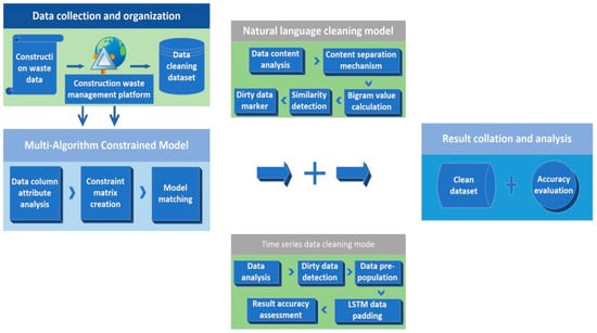
Figure 1.
Overall algorithm flow chart.
2.2. Multi-Algorithm Constrained Model
Data cleaning can accurately find and correct identifiable errors in the data; however, too many data types will have a greater impact on the data cleaning effect. Therefore, solving the problem of data quality reduction caused by the diversity of data types is the main problem of data cleaning technology.
Herein, data cleaning of construction waste data was carried out, and large errors were found in the cleaning results. After analyzing the error of the construction waste data detection results, the difference in data attributes in the construction waste data of the same module (i.e., natural language data and time series data exist at the same time) leads to confusion in the matching of the cleaning model and data during cleaning. As a result, the cleaned data still possess “dirty data”. Therefore, the accurate matching of data cleaning content and data cleaning model is the premise for obtaining high-quality data.
In this study, the TOPSIS algorithm in MADM was employed to construct a multi-algorithm constraint model. Among them, the TOPSIS method, which is a multi-attribute decision-making method for sorting limited alternatives, was proposed by Hwang and Yoon. The principle of this method is to standardize the problem impact index, obtain the distance between the solution and the index’s positive and negative ideal solutions through the distance calculation method, and finally select the solution that is close to the positive ideal solution but far away from the negative ideal solution as the optimal solution. Accordingly, the final match between the data cleaning model and the data cleaning content is achieved by calculating the degree of closeness. The specific technical route is shown in Figure 2.
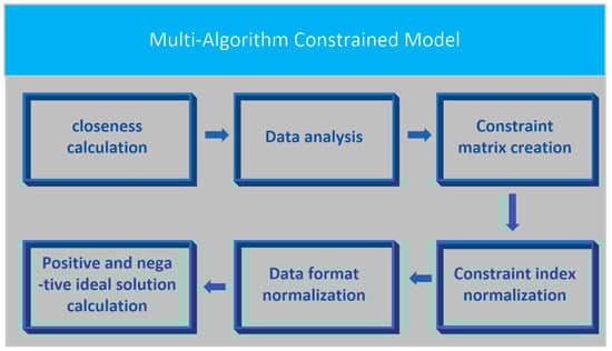
Figure 2.
Multi-algorithm constrained model technology flowchart.
To obtain the attribute constraint matrix of the construction waste data, the initial construction waste data set was analyzed. By obtaining the column data type of the dataset, a multi-attribute constraint matrix X was constructed, as shown in Equation (1) [15].
In the formula, each scheme in the scheme set of the multi-attribute decision scheme is .
To solve the problem of different trends of data indicators, the identification and normalization of indicator trends were carried out. There are four indicator trend types, as shown in Table 1 [16].

Table 1.
Examples of the indicator trend type.
After normalization, to realize the unification of the data format, the data was normalized, as shown in Equation (2) [17]. Finally, the normalized matrix Z was obtained, as shown in Equation (3).
In the equation: ; j = .
Based on the standardized matrix Z, the positive ideal solution and negative ideal solution of each index were obtained, as shown in Equations (4) and (5):
Finally, the Manhattan distance was used to calculate the distance between the object and the optimal value and the worst value [18].
According to the obtained distance, the corresponding closeness and index ranking were obtained, as shown in Equation (6).
In the equation, is the matching degree between the cleaning model and the data; the smaller the value, the lower the match between the cleaning model and the data.
2.3. Natural Language Data Cleaning Model
At present, N-gram is the main algorithm for cleaning natural language data. The N-gram algorithm is a language model for the continuous recognition of a large vocabulary. The core idea of this algorithm is to assume that words in the content have a certain probability of occurrence. Thus, the preprocessed content is segmented, sliding cutting is performed according to a fixed size window, and a sequence of byte fragments of length N is fabricated. The frequency of occurrence of each byte fragment sequence is counted and filtered according to the preset threshold, and the probability of occurrence of the entire record is obtained by counting the probability of occurrence of byte fragments. However, as the natural language data of construction waste contain spatial location data and main cleaning data, the original repetition of spatial location data leads to the inaccurate similarity of the final data [19]. To solve this problem, a natural language data cleaning model based on the N-Gran algorithm was proposed in this study. Through the content separation mechanism designed in the model, the integrity and accuracy of the natural language cleaning of construction waste were improved. Figure 3 shows the overall technical flowchart of the natural language data cleaning model:
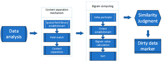
Figure 3.
Overall technical roadmap of the natural language data cleaning model.
First, the construction waste data were analyzed, which revealed spatial location data in the data, and potential repeats of spatial location data in different data, resulting in incorrect similarity during cleaning [20]. Therefore, the content separation mechanism was adopted to obtain the main cleaning data set [21].
After obtaining the main cleaning data set, to ensure the validity of the data, the occurrence probability distribution between the words in the construction waste data record must be assumed to obey the n-1 order Markov model.
To markedly improve the data cleaning effect, the N value must be selected [22]. As the number of times of construction waste natural language data vocabulary composition is two2, the N value of two can maximize detection accuracy. The probability of occurrence of construction waste data records is set as [23,24,25,26,27]. The equation is shown in (7):
To calculate the repeatability of the data, similarity detection was performed on the data. The similarity detection algorithm adopts the Levenshtein Distance. The Levenshtein Distance was proposed by Levenshtein et al., and is a distance-based similar duplicate record matching algorithm. The core idea of this algorithm is to compare and analyze the two records, A and B, to find the difference between the two data characters. Assuming that the characters can be converted, the insertion, deletion, and replacement operations that must go from character A to character B must be recorded. The number of operations per operation is set to 1, and the number of operations required to go from A to B, which is called the edit distance, is counted. The fewer operations required, the higher the similarity. Accordingly, the similarity between the data was obtained by quantifying the similarity of the strings.
2.4. Time Series Data Cleaning Model
As the construction waste data are time series data, they are comparable to the same period data. Therefore, commonly used detection algorithms are used to construct the time series data for construction waste. For example, the detection algorithm based on the DBScan cluster is mainly based on the form of density detection, which cannot effectively utilize the time series attributes of the data. Furthermore, the construction waste data are large-span time series data [28]. Thus, the detection results of the data are poor. The statistical-based detection algorithm can have a better data detection effect through the comparative analysis of the time series [29,30]. Among them, the Pauta criterion is the most common and convenient method based on statistical detection algorithms. This method primarily seeks to determine whether all datasets differ from the dataset mean by more than three times the standard deviation. As this method is simple and convenient, and has the characteristics of better experimental results when the amount of data is large, the Pauta criterion method in statistics was adopted to detect and mark the time series data of the construction waste.
To improve the effectiveness of the filling results of the construction waste time series data, the data were divided according to the construction waste time series data attributes. The Laida criterion was used for the detection, and the sliding window was used for marking [31,32]. To solve the problem of long data time series of construction waste spatiotemporal data, the method of “detection first and then filling” was adopted for cleaning. As shown in Equation (8), the construction waste time series data set was pre-filled.
To achieve accurate data filling, the LSTM algorithm was used for detection. LSTM is a recurrent neural network that was proposed by Hochreiter in 1997. This algorithm is a special network form of RNN that converts the tanh layer in the traditional recurrent neural network to include storage units and gates, modifying the structure of the memory cell, thereby overcoming the traditional RNN gradient diffusion and explosion problems. Its main process is described below.
First, the construction waste information that can be transmitted to the memory unit, which is controlled by the sigmoid function in the forget gate, is determined [33]. A value between 0 and 1 to is assigned based on the output at time t-1 and the input at time t. is mainly used to determine whether to fully or partially transmit the construction waste information learned at the previous instance [34]. The sigmoid function equation is shown in (9)
The equation is shown in (10):
where represents the forget gate, with a value range of [0, 1]; the symbol represents the sigmoid function; and ∈, ∈, ∈; 1 indicates “completely reserved”, 0 indicates “totally abandoned”.
The next step involves the generation of the new construction waste data required for the update [35,36,37]. This step mainly depends on two aspects: the input gate uses the sigmoid function to decide which construction waste data must be updated; the new candidate value generated by the tanh layer is stored in the cell state [38], as shown in Equations (11)–(13).
where represents the input gate, and the value range is [0, 1].
An update of the old unit must be performed. First, the old cell state must be multiplied by to forget the unwanted construction waste data. Thereafter, * must be added to the result to obtain the candidate value [39]. The main Equation (14) is shown below:
Finally, the output of the model is determined, the initial output through a sigmoid layer is obtained, the tanh layer is used to perform the shrinking operation, the sigmoid tanh in pairs is multiplied, and a clean data set is obtained [40,41,42,43]. The and equations (i.e., (15) and (16)) are shown below:
where is the output gate, and its value range is “(0, 1)”.
3. Results and Evaluation
3.1. Experimental Data
Construction waste is the collective term for muck, waste concrete, waste masonry, and other wastes generated during production activities related to demolition, construction, decoration, repair, and other construction activities. According to the source classification, construction waste can be divided into engineering muck, engineering mud, engineering waste, demolition waste and decoration waste, etc. Based on the composition, construction waste can be divided into muck, concrete block, crushed stone, brick and tile fragments, waste mortar, mud, asphalt blocks, waste plastics, waste metals, waste bamboo and wood, etc. The experimental data include all types of construction waste, and the data quality of the overall construction waste data is shown to be improved.
The main source of the data in this study is the construction waste management platform. Based on data collection from 35 pilot cities, a total of 5961 pieces of data were collected. According to the classification of the platform function modules, the data were divided into nine categories, as shown in Figure 4.
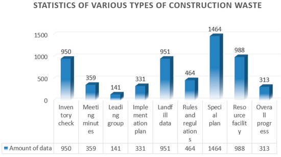
Figure 4.
Statistics of various types of construction waste.
(1) Inventory inspection data: Statistics on the amount of data retained in construction waste. The data mainly include total garbage stock, engineering dregs, engineering mud, etc. (2) Meeting minutes data: relevant meeting minutes on construction waste management. The data mainly include the theme of the conference, the participants, and an overview of the content of the conference. (3) Leading group data: information on the leading groups of each pilot city. The data mainly include city, contact person, phone number, etc. (4) Implementation plan data: document records issued by construction waste management. The data mainly include city, time, program type, etc. (5) Landfill data: statistical data of landfill information. The data mainly include city, time, and project name. (6) Rules and regulations data: statistical data of the construction waste management work rules and regulations. The data mainly include city, time, number, etc. (7) Special planning data: statistical data of construction waste treatment planning documents. The main contents include city, time, planning type, etc. (8) Resource facility data: statistical data for information related to the resource facility. The data mainly include city, time, project name, etc. (9) Overall progress data: statistical data on the completion of construction waste treatment work. The data mainly include city, time, and work ratio.
3.2. Experimental Results
The algorithm proposed in this study detects the construction waste test data; the detection results are shown in Table 2.
Table 2.
The algorithm detection results.
Nine categories of data were selected as the detection data source to test the algorithm proposed in this study, the natural language data cleaning model, and the time series data cleaning model. Among them, the algorithm detected 1846 pieces of dirty data as a whole, including 1733 pieces of correct dirty data, 113 pieces of incorrect dirty data, and 37 pieces of missing data. Herein, the recall rate and precision rate were used to represent the accuracy of the algorithm. The precision rate was 93.88% and the recall rate was 97.90%.
The amount of dirty data in each module of the natural language data cleaning model was 1062, of which 940 were correct for the detection of dirty data, 122 were incorrect for the detection of dirty data, and 78 were missing overall. Herein, the recall rate and precision rate were used to represent the accuracy of the algorithm. The precision rate was 88.65% and the recall rate was 92.33%.
The number of dirty data detected by each module of the time series data cleaning model was 1335, of which 1184 were correct for the detection of dirty data, 151 were incorrect for the detection of dirty data, and 91 were missing overall. Herein, the recall rate and precision rate were used to represent the accuracy of the algorithm. The precision rate was 88.68% and the recall rate was 92.86%.
3.3. Result Analysis
To further reflect the advanced nature of the algorithm, the cleaning results of the algorithm were compared with those of a single cleaning model. The recall rate and precision rate were used to evaluate the cleaning accuracy of the construction waste natural language, and the average root mean square error (RMSE) and average MAPE indicators were used to evaluate the filling accuracy of the construction waste time series data of this algorithm.
3.3.1. Construction Waste Natural Language Data
The landfill data were employed as the experimental data, and 800 pieces of data were selected as the sample data. The similarity was calculated using the Smith–Waterman (S-W) algorithm and the Levenshtein distance algorithm, and the corresponding recall and precision were calculated. The comparison results are shown in Table 3.
Table 3.
Accuracy comparison results.
In terms of precision, the cleaning accuracy increased from 0.875 to the highest of 0.961. The accuracy of the Levenshtein distance algorithm was as low as 0.667 and as high as 0.78. The precision of the Smith–Waterman algorithm ranged from 0.7 (the lowest) to 0.807 (the highest). The maximum difference between the accuracy of the cleaning algorithm and the Levenshtein distance algorithm was 0.208, and the minimum difference was 0.178. The maximum difference with the accuracy of the Smith–Waterman algorithm was 0.175, and the minimum difference was 0.137. The comparison results are shown in Table 4.
Table 4.
The full comparison results.
In terms of recall, the cleaning accuracy increased from 0.8742 to the highest of 0.932. The accuracy of the Levenshtein distance algorithm ranged from 0.687 (the lowest) to 0.764 (the highest). The precision of the Smith–Waterman algorithm ranged from 0.727 (the lowest) to 0.782 (the highest).
The maximum difference between the accuracy of the cleaning algorithm proposed in this study and the Levenshtein distance was 0.168, the minimum difference was 0.146, the maximum difference between the precision of the Smith–Waterman algorithm was 0.15, and the minimum difference was 0.115.
Figure 5 and Figure 6 show the comparison of recall and precision changes. In this study, the method of sorting and then cleaning was adopted, and the accuracy of sorting was followed by further matching, which could markedly improve the accuracy of data cleaning. It not only fully meets the requirements of data cleaning technology, but also continues to increase with the continuous increase in data volume, and finally approaches a threshold.
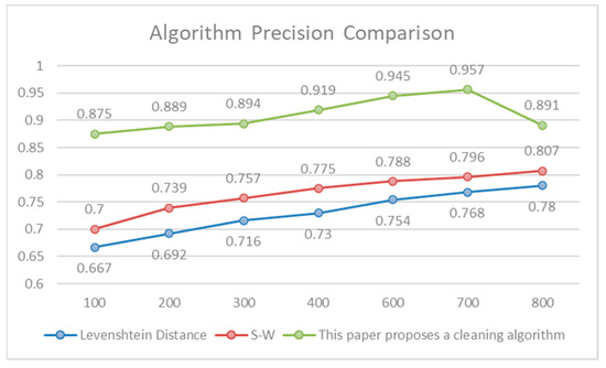
Figure 5.
Algorithm Precision Comparison.
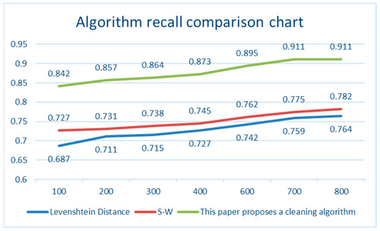
Figure 6.
Algorithm recall comparison chart.
3.3.2. Construction Waste Data Time Series Data
Using RMSE and MAPE as evaluation indicators, the data cleaning results of the time series data cleaning model proposed herein and the traditional LSTM data cleaning model were compared. The indicator value is inversely proportional to the precision of the data. As shown in Table 5, five types of data, including total waste, engineering muck, engineering mud, engineering waste, and demolition waste were tested.
Table 5.
Accuracy comparison data table.
Among the RMSE indicators, the engineering mud data had the highest improvement, with a decrease of 14.25, while the demolition garbage data had the lowest improvement, with a decrease of 9.253. Among the MAPE indicators, the engineering mud data had the highest improvement, with a decrease of 8.88, while the engineering waste data had the lowest improvement, with a decrease of 7.3. In each module, the time series data cleaning model proposed herein markedly improved the accuracy of RMSE and MAPE compared with that of the traditional LSTM data cleaning model.
The accuracy was compared with the average RMSE and MAPE. As shown in Table 6, the improved LSTM filling model had a higher accuracy.
Table 6.
Comparison Table of Average Precision.
As shown in Figure 7, the average accuracy evaluation of the model was compared. The improved LSTM filling model proposed herein is more conducive to the improvement of data quality than that of the traditional LSTM filling model.
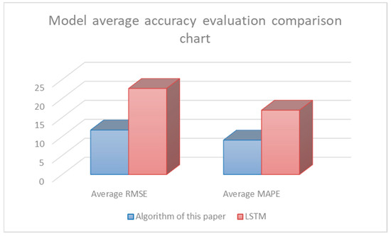
Figure 7.
Algorithm average recall comparison chart.
3.3.3. Comparative Analysis of the Cleaning Effect
To reflect the overall improvement of the effect of the algorithm, the recall and precision rates of a single algorithm, a single cleaning model and the algorithm proposed herein are outlined, as shown in Table 7.
Table 7.
Average accuracy comparison data sheet.
Based on the N-gram algorithm, the natural language precision rate was 81.73%, and the natural language recall rate was 84.56%; the precision rate of the time series data was empty, and the recall rate of time series data was empty. After data cleaning based on the N-gram algorithm + natural language data cleaning model, the precision rate of natural language increased by 6.92% to 88.65%, and the recall rate of natural language increased by 7.77% to 92.33%. The precision of the time series data was empty, and the recall of time series data was empty. Based on the N-gram algorithm + natural language data cleaning model + multi-algorithm constraint model + time series data cleaning model, the natural language precision rate of the algorithm increased by 13.14% to 94.87%; the natural language recall rate increased by 13.34%, reaching 97.90%; the precision of the time series data was 97.13%, and the recall rate of the time series data was 98.67%.
4. Discussion
A multi-type construction waste data cleaning algorithm was proposed in this study. According to the diversity of the construction waste data, a natural language data cleaning model and a time series data cleaning model were designed to achieve accurate and complete cleaning of multi-type construction waste data. Comparative experiments with various algorithms revealed that our algorithm has certain advantages. Below, the overall structure and advantages of the algorithm, including the design and advantages of the cleaning model, the design and advantages of the multi-constraint combinatorial model, and the limitations of the algorithm, are discussed.
4.1. Cleaning Model Design and Advantages
The concept of data cleaning has a long history. For data cleaning research, scholars from various countries have proposed different cleaning algorithms. According to the cleaning content, these algorithms can be divided into time series data cleaning algorithms and natural language data cleaning algorithms. Among them, the algorithms for time series data cleaning mainly include the K-means clustering algorithm, Bayesian network, density-based local outlier factor detection algorithm, Detection algorithm based on data flow, etc. [44,45,46]. In contrast, the algorithms for natural language data cleaning mainly include the SNM algorithm, MPN algorithm, Distance based algorithm for similarity detection, etc. [47,48]. At present, most algorithms only perform data cleaning for a single data set; however, construction waste data are diverse, and the data include natural language data and numerical data, which leads to a poor cleaning effect of a single algorithm for construction waste data. According to the diversity of construction waste data, a natural language data cleaning model and a time series data cleaning model were proposed herein to ensure the accuracy and integrity of data cleaning.
4.2. Design and Advantages of the Multi-Algorithm Constrained Models
Construction waste data are diverse and mixed. Thus, in the same type of data, the data attributes of each piece of data include natural language data and time series data, and the proportion of natural language data and time series data in each piece of data is different. At present, there are many algorithms for data cleaning, such as the improved PNRS algorithm, Original operator cleaning algorithm based on similar connection, Cleaning algorithm based on support vector machine (SVM), etc. [49,50,51]. However, when data cleaning is performed, the cleaning model cannot be selected, which is a problem. Accordingly, this study sought to propose a multi-algorithm constraint model, which mainly uses the idea of MADM to achieve accurate matching between the data cleaning model and the data cleaning range, and finally realize the “one-to-one” cleaning mode, thereby markedly improving the construction waste data cleaning accuracy.
4.3. Limitations of the Algorithm
Based on experiments, the algorithm proposed herein is effective; however, some problems still exist. For example, although the algorithm cleans the natural language data and time series data when cleaning the construction waste data, the spatial location data existing in the natural language cannot be cleaned. Thus, further research on the spatial location data should be carried out in the future. Moreover, as the experimental data were collected at a certain period of time, there is still room for further expansion in the number of data sets. The effectiveness of the algorithm can be further verified by expanding the experimental data sets in the future.
5. Conclusions
Owing to the multi-type characteristics of construction waste data, this study sought to propose a data cleaning algorithm based on multi-type construction waste. The algorithm is mainly composed of three parts: the multi-algorithm constraint model, the natural language data cleaning model, and the time series data cleaning model. Based on traditional data cleaning, multiple cleaning models were combined, which effectively alleviated the poor cleaning effect caused by the many types of construction waste data. According to the test results of the experimental data set, the precision and recall of the algorithm reached 93.87% and 97.90%, respectively, indicating its ability to clean dirty data relatively completely and accurately. From the comparison experiment, the algorithm herein has remarkable improvement in precision and recall compared to that of a single model. Compared with the natural language data cleaning model, the precision and recall increased by 5.23% and 5.57%, respectively. Compared with the time series data cleaning model, the patent checking and recall rates increased by 5.2% and 5.04%, respectively.
In summary, the proposed algorithm has great improvement in cleaning integrity and accuracy, and its specific advantages are as follows.
The multi-algorithm constraint model realizes the matching between the cleaning algorithm and the cleaning content, thereby accurately matching the cleaning model and the cleaning content, and effectively improving the effect of data cleaning.
For traditional natural language data cleaning, combined with the characteristics of construction waste data, the spatial location data and general data are isolated, which remarkably improves the cleaning efficiency.
Based on the large vacancy of the time series data for construction waste data, the pre-fill method is used to preprocess the data set, which effectively improves the accuracy of data filling.
Although the experiments demonstrated that our algorithm has certain effectiveness, it still has some problems. For example, through further analysis of the construction waste data, some dirty data were found in the spatial location data. In the follow-up work, this problem will be evaluated according to the dirty data processing technology of spatial location information. Due to the increasing number of multi-type data, single data cannot meet the requirements of the data cleaning technology, and multi-type algorithms will be the main cleaning methods for future data cleaning algorithms.
Author Contributions
P.W. designed this study. P.W. performed the data collection, processing, and analysis. Q.S. and C.L. and Y.B. provided the logging results and micro-seismic data for this work. Y.L. supervised this work and offered continued guidance throughout this work. P.W. wrote this manuscript. The manuscript was edited by Y.L. All authors have read and agreed to the published version of the manuscript.
Funding
This work was supported by the National Key Research and Development Program of China (2018YFC0706003).
Acknowledgments
The authors thank the anonymous reviewers for their constructive comments and suggestions that helped improve the manuscript.
Conflicts of Interest
The authors declare that they have no conflict of interest.
References
- Ma, X.C.; Luo, W.J.; Yin, J. Review and feasibility analysis of prefabricated recycled concrete structure. In Proceedings of the IOP Conference Series: Earth and Environmental Science, Qingdao, China, 5–7 June 2020; IOP Publishing: Bristol, UK, 2020; Volume 531, p. 012052. [Google Scholar]
- Long, H.; Xu, S.; Gu, W. An abnormal wind turbine data cleaning algorithm based on color space conversion and image feature detection. Appl. Energy 2022, 311, 118594. [Google Scholar] [CrossRef]
- Hwang, J.S.; Mun, S.D.; Kim, T.J. Development of Data Cleaning and Integration Algorithm for Asset Management of Power System. Energies 2022, 15, 1616. [Google Scholar] [CrossRef]
- Candelotto, L.; Grethen, K.J.; Montalcini, C.M. Tracking performance in poultry is affected by data cleaning method and housing system. Appl. Anim. Behav. Sci. 2022, 249, 105597. [Google Scholar] [CrossRef]
- Gao, F.; Li, J.; Ge, Y. A Trajectory Evaluator by Sub-tracks for Detecting VOT-based Anomalous Trajectory. ACM Trans. Knowl. Discov. Data TKDD 2022, 16, 1–19. [Google Scholar] [CrossRef]
- Liu, H.; Shah, S.; Jiang, W. On-line outlier detection and data cleaning. Comput. Chem. Eng. 2004, 28, 1635–1647. [Google Scholar] [CrossRef]
- Corrales, D.C.; Ledezma, A.; Corrales, J.C. A case-based reasoning system for recommendation of data cleaning algorithms in classification and regression tasks. Appl. Soft Comput. 2020, 90, 106180. [Google Scholar] [CrossRef]
- Luo, Z.; Fang, C.; Liu, C.; Liu, S. Method for Cleaning Abnormal Data of Wind Turbine Power Curve Based on Density Clustering and Boundary Extraction. IEEE Trans. Sustain. Energy 2021, 13, 1147–1159. [Google Scholar] [CrossRef]
- Ji, C.B.; Duan, G.J.; Zhou, J.Y. Equipment Quality Data Integration and Cleaning Based on Multiterminal Collaboration. Complexity 2021, 2021, 5943184. [Google Scholar] [CrossRef]
- Yuan, J.; Zhou, Z.; Huang, K. Analysis and evaluation of the operation data for achieving an on-demand heating consumption prediction model of district heating substation. Energy 2021, 214, 118872. [Google Scholar] [CrossRef]
- Shi, X.; Prins, C.; Van Pottelbergh, G.; Mamouris, P.; Vaes, B.; De Moor, B. An automated data cleaning method for Electronic Health Records by incorporating clinical knowledge. BMC Med. Inform. Decis. Mak. 2021, 21, 267. [Google Scholar] [CrossRef]
- Dutta, V.; Haldar, S.; Kaur, P. Comparative Analysis of TOPSIS and TODIM for the Performance Evaluation of Foreign Players in Indian Premier League. Complexity 2022, 2022, 9986137. [Google Scholar] [CrossRef]
- Fa, P.; Qiu, Z.; Wang, Q.E.; Yan, C.; Zhang, J. A Novel Role for RNF126 in the Promotion of G2 Arrest via Interaction With 14–3-3σ. Int. J. Radiat. Oncol. Biol. Phys. 2022, 112, 542–553. [Google Scholar] [CrossRef] [PubMed]
- Zeng, B.; Sun, Y.; Xie, S. Application of LSTM algorithm combined with Kalman filter and SOGI in phase-locked technology of aviation variable frequency power supply. PLoS ONE 2022, 17, e0263634. [Google Scholar] [CrossRef]
- Fang, K.; Wang, T.; Zhou, X. A TOPSIS-based relocalization algorithm in wireless sensor networks. IEEE Trans. Ind. Inform. 2021, 18, 1322–1332. [Google Scholar] [CrossRef]
- Shohda, A.M.A.; Ali, M.A.M.; Ren, G. Sustainable Assignment of Egyptian Ornamental Stones for Interior and Exterior Building Finishes Using the AHP-TOPSIS Technique. Sustainability 2022, 14, 2453. [Google Scholar] [CrossRef]
- Zhang, X.; Xu, Z. Extension of TOPSIS to multiple criteria decision making with Pythagorean fuzzy sets. Int. J. Intell. Syst. 2014, 29, 1061–1078. [Google Scholar] [CrossRef]
- Polcyn, J. Determining Value Added Intellectual Capital (VAIC) Using the TOPSIS-CRITIC Method in Small and Medium-Sized Farms in Selected European Countries. Sustainability 2022, 14, 3672. [Google Scholar] [CrossRef]
- Liu, Y.; Wang, L.; Shi, T. Detection of spam reviews through a hierarchical attention architecture with N-gram CNN and Bi-LSTM. Inf. Syst. 2022, 103, 101865. [Google Scholar] [CrossRef]
- Korkmaz, M.; Kocyigit, E.; Sahingoz, O.K. Phishing web page detection using N-gram features extracted from URLs. In Proceedings of the 2021 3rd International Congress on Human-Computer Interaction, Optimization and Robotic Applications (HORA), Ankara, Turkey, 11–13 June 2021; IEEE: New York, NY, USA, 2021; pp. 1–6. [Google Scholar]
- Chaabi, Y.; Allah, F.A. Amazigh spell checker using Damerau-Levenshtein algorithm and N-gram. J. King Saud Univ.-Comput. Inf. Sci. 2021, 34, 6116–6124. [Google Scholar] [CrossRef]
- Ghude, T. N-gram models for Text Generation in Hindi Language. In ITM Web of Conferences; EDP Sciences: Les Ulis, France, 2022; Volume 44, p. 03062. [Google Scholar]
- Song, Y. Zen 2.0: Continue training and adaption for n-gram enhanced text encoders. arXiv 2021, arXiv:2105.01279. [Google Scholar]
- Zhu, L. A N-gram based approach to auto-extracting topics from research articles. J. Intell. Fuzzy Syst. 2021. preprint. [Google Scholar]
- Tian, J. Improving Mandarin End-to-End Speech Recognition with Word N-Gram Language Model. IEEE Signal Process. Lett. 2022, 29, 812–816. [Google Scholar] [CrossRef]
- Sester, J.; Hayes, D.; Scanlon, M. A comparative study of support vector machine and neural networks for file type identification using n-gram analysis. Forensic Sci. Int. Digit. Investig. 2021, 36, 301121. [Google Scholar] [CrossRef]
- Aouragh, S.L.; Yousfi, A.; Laaroussi, S. A new estimate of the n-gram language model. Procedia Comput. Sci. 2021, 189, 211–215. [Google Scholar] [CrossRef]
- Szymborski, J.; Emad, A. RAPPPID: Towards generalizable protein interaction prediction with AWD-LSTM twin networks. Bioinformatics 2022, 38, 3958–3967. [Google Scholar] [CrossRef] [PubMed]
- Wang, X.; Xu, N. Meng X; Prediction of Gas Concentration Based on LSTM-Light GBM Variable Weight Combination Model. Energies 2022, 15, 827. [Google Scholar] [CrossRef]
- Liu, M.Z.; Xu, X.; Hu, J. Real time detection of driver fatigue based on CNN-LSTM. IET Image Process. 2022, 16, 576–595. [Google Scholar] [CrossRef]
- Akhter, M.N.; Mekhilef, S.; Mokhlis, H. An Hour-Ahead PV Power Forecasting Method Based on an RNN-LSTM Model for Three Different PV Plants. Energies 2022, 15, 2243. [Google Scholar] [CrossRef]
- Jogunola, O.; Adebisi, B.; Hoang, K.V. CBLSTM-AE: A Hybrid Deep Learning Framework for Predicting Energy Consumption. Energies 2022, 15, 810. [Google Scholar] [CrossRef]
- Chung, W.H.; Gu, Y.H.; Yoo, S.J. District heater load forecasting based on machine learning and parallel CNN-LSTM attention. Energy 2022, 246, 123350. [Google Scholar] [CrossRef]
- Tao, C.; Lu, J.; Lang, J. Short-Term forecasting of photovoltaic power generation based on feature selection and bias Compensation–LSTM network. Energies 2021, 14, 3086. [Google Scholar] [CrossRef]
- Ordóñez, F.J.; Roggen, D. Deep convolutional and lstm recurrent neural networks for multimodal wearable activity recognition. Sensors 2016, 16, 115. [Google Scholar] [CrossRef]
- Zhang, S. Fusing geometric features for skeleton-based action recognition using multilayer LSTM networks. IEEE Trans. Multimed. 2018, 20, 2330–2343. [Google Scholar] [CrossRef]
- Zhao, F.; Feng, J.; Zhao, J. Robust LSTM-autoencoders for face de-occlusion in the wild. IEEE Trans. Image Process. 2017, 27, 778–790. [Google Scholar] [CrossRef] [PubMed]
- Liu, Q.; Zhou, F.; Hang, R. Bidirectional-convolutional LSTM based spectral-spatial feature learning for hyperspectral image classification. Remote Sens. 2017, 9, 1330. [Google Scholar] [CrossRef]
- Wentz, V.H.; Maciel, J.N.; Gimenez Ledesma, J.J. Solar Irradiance Forecasting to Short-Term PV Power: Accuracy Comparison of ANN and LSTM Models. Energies 2022, 15, 2457. [Google Scholar] [CrossRef]
- Banik, S.; Sharma, N.; Mangla, M. LSTM based decision support system for swing trading in stock market. Knowl.-Based Syst. 2022, 239, 107994. [Google Scholar] [CrossRef]
- Hwang, J.S.; Kim, J.S.; Song, H. Handling Load Uncertainty during On-Peak Time via Dual ESS and LSTM with Load Data Augmentation. Energies 2022, 15, 3001. [Google Scholar] [CrossRef]
- Rosas, M.A.T.; Pérez, M.R.; Pérez, E.R.M. Itineraries for charging and discharging a BESS using energy predictions based on a CNN-LSTM neural network model in BCS, Mexico. Renew. Energy 2022, 188, 1141–1165. [Google Scholar] [CrossRef]
- Maleki, S.; Maleki, S.; Jennings, N.R. Unsupervised anomaly detection with LSTM autoencoders using statistical data-filtering. Appl. Soft Comput. 2021, 108, 107443. [Google Scholar] [CrossRef]
- Sinaga, K.P.; Yang, M.S. Unsupervised K-means clustering algorithm. IEEE Access 2020, 8, 80716–80727. [Google Scholar] [CrossRef]
- Marcot, B.G.; Penman, T.D. Advances in Bayesian network modelling: Integration of modelling technologies. Environ. Model. Softw. 2019, 111, 386–393. [Google Scholar] [CrossRef]
- Liu, Y.; Lou, Y.; Huang, S. Parallel algorithm of flow data anomaly detection based on isolated forest. In Proceedings of the 2020 International Conference on Artificial Intelligence and Electromechanical Automation (AIEA), Tianjin, China, 26–28 June 2020; IEEE: New York, NY, USA, 2020; pp. 132–135. [Google Scholar]
- Zhang, J.Z.; Fang, Z.; Xiong, Y.J.; Yuan, X.Y. Optimization algorithm for cleaning data based on SNM. J. Cent. South Univ. Sci. Technol. 2010, 41, 2240–2245. [Google Scholar]
- Martini, A.; Kuper, P.V.; Breunig, M. Database-Supported Change Analysis and Quality Evaluation of Openstreet map Data. ISPRS Ann. Photogramm. Remote Sens. Spat. Inf. Sci. 2019, 4, 535–541. [Google Scholar] [CrossRef]
- Save, A.M.; Kolkur, S. Hybrid Technique for Data Cleaning. Int. J. Comput. Appl. 2014, 975, 8887. [Google Scholar]
- Chaudhuri, S.; Ganti, V.; Kaushik, R. A primitive operator for similarity joins in data cleaning. In Proceedings of the 22nd International Conference on Data Engineering (ICDE’06), Atlanta, GA, USA, 3–7 April 2006; IEEE: New York, NY, USA, 2006; p. 5. [Google Scholar]
- Tang, J.; Li, H.; Cao, Y. Email data cleaning. In Proceedings of the Eleventh ACM SIGKDD International Conference on Knowledge Discovery in Data Mining, Chicago, IL, USA, 21–24 August 2005; pp. 489–498. [Google Scholar]


Publisher’s Note: MDPI stays neutral with regard to jurisdictional claims in published maps and institutional affiliations. |
© 2022 by the authors. Licensee MDPI, Basel, Switzerland. This article is an open access article distributed under the terms and conditions of the Creative Commons Attribution (CC BY) license (https://creativecommons.org/licenses/by/4.0/).