Does Retirement Affect Household Energy Consumption Structure? Evidence from a Regression Discontinuity Design

Abstract

Whether retirement can affect household energy consumption structure is an interesting topic in relation to environment and aging. Based on China’s Urban Household Survey (UHS) data, we adopt a regression discontinuity design (RDD) to identify this causal effect. The empirical results show that households suddenly reduce their overall energy consumption by about 2.5 percent when they retire. Specifically, retirement greatly reduces household energy consumption expenditure related to work by about 55.4 percent, reduces non-durable products by about 12.1 percent, and reduces dining out consumption by about 55.3. Moreover, the mechanism analysis shows that householders reduce their social activities after retirement and spend much more time at home, so that the direct energy consumed increases and the indirect energy consumed decreases. The reduction in household non-durable energy consumption expenditure after retirement is closely related to the reduction in work-related energy consumption. Our conclusion has passed a series of validity tests and robustness tests. Our finding implies that it is valuable to design energy policies by considering these causal effects.

1. Introduction

According to China’s National Bureau of Statistics, in 2018, China’s total energy consumption reached 4.64 billion tons of standard coal, up by 3.3 percent over 2017, and it remains the world’s largest energy consumer. Considering that growing energy consumption is putting increasing pressure on environmental pollution and global warming [1], scholars have studied many factors that may lead to changes in energy consumption, among which energy consumption in urban areas has drawn more attention because of increasing urbanization [2] and economic growth [3], especially in the context of China [4,5,6,7,8,9]. The study found that the urban contribution to China’s total commercial energy uses was enormous—84% in 2006 [4]. However, with a path of rapid economic growth and increasing urbanization in China (urban permanent residents account for 59.58 percent of the total population in 2018), China’s residents’ total energy consumption and the urban share of energy usage are showing a sustained increasing trend, and the peak point may come in 2030 because of the overall slowing of population growth [10]. Scholars have argued that based on the interpretation of the final users’ needs being the driver of increasing energy use and related emissions [11,12,13], a household consumption-based perspective in this study to allocate the energy use directly and indirectly should be considered [14]. Several papers have worked from the household perspective [8,15,16,17,18,19,20,21,22,23,24,25]; however, the household attributes affecting energy consumption structure have rarely been studied in the literature because of methodological issues, their complexity, and the cost and non-availability of individual disaggregated data [26,27,28].

Meanwhile, population aging has become a global phenomenon, and the trend is expected to continue in the foreseeable future [29]. In China, the world’s most populous nation, the proportion of population aged 65 and above is projected to triple from 9.6% in 2015 to 27.6% in 2050, and the old-age dependency ratio will increase from 0.13 to 0.47 during the same period [30]. Population aging can have huge impacts on economic outcomes from the macro to micro levels in terms of environment and energy use. At the macro level, the existing literature has measured the aged population using the share of population above 60 or 65 years old, and found that an aging population can lead to residential electricity and city gas consumption increases in Japan [31]. It could also offset the likelihood of the UK government meeting its energy targets, not only by increasing domestic thermal comfort, but also potentially by increasing consumption in the home and other consumer lifestyle choices [32]. The effect of an aged population and CO₂ emission could be negative [33], positive [34] or quadratic [35] in the context of road transportation using different methods. However, at the micro level, most of the existing literature focuses on household energy consumption behavior [18,20,21], and elderly households (including one-person households with an age over 60) spend more than other households because of their higher expense on fuel and light in Japan [36]. However, few papers study the effects of population aging on household energy consumption in the context of China at the household level.

Based on the above background, this study attempts to explore the impact of retirement on the energy consumption structure at the micro-household level, in order to provide constructive suggestions on how to better achieve energy conservation and emission reduction in China. However, the existing literature defines an aging population as that aged over 60 or 65, and this may clash with certain policies, especially in the context of China, where the mandatory retirement age for male workers in the formal sectors (including government, public sectors, state-owned enterprises (SOEs), and collectively owned enterprises (COEs)) is also 60. Consumers may change their energy consumption due to the retirement policy, not just based on their aging status, suggesting that to separate these two different but mixed mechanisms is quite important for policy-makers to improve household energy consumption structure. Scholars have found that consumption expenditure declines sharply at the time of retirement, and the mechanism and underlying theory have drawn much attention [37,38]. However, the relationship between the retirement of the household leader and the household energy consumption is still an unsolved question. In fact, the establishment of a causal link between retirement and household energy consumption faces two challenges: First, household energy consumption may not be well defined. To the best of our knowledge, data of energy use and CO₂ emission at the household level are rare, especially in terms of the different household energy consumption structures. Second, retirement decisions often depend on income [39,40], and household energy consumption depends on income [19,41], so retirement is an endogenous decision variable that incurs inconsistent results under conventional regression methods.

In response, we implemented a regression discontinuity design method (RDD) on China’s Urban Household Survey (UHS) data to establish a causal link, which enables us to handle the two above-mentioned challenges. The research contributions of this paper are as follows: (1) Using data from the UHS, which include detailed information on each household consumption item, to analyze the impact of retirement on household energy consumption structure at the micro level, filling the gap in the literature. (2) According to the household consumption amount of each product provided by UHS data, combined with product attributes, we construct indicators of different types of household energy consumption. (3) An understanding of causal factors based on China’s retirement policy not only reduces the endogeneity problem, but also results in the exogenous threshold age of retirement that is needed in RDD, making the estimation results in this paper more accurate. Furthermore, RDD still obtains consistent results even if household retirement decisions are dependent on energy consumption.

Our empirical results indicate that the energy consumptions of Chinese households do respond to the retirement of the husband; however, we found different marginal effect in terms of the components of total energy consumption. The retirement of the husband can reduce a household’s overall energy consumption. The effect is mostly on the work-related energy consumption, and when it comes to other energy forms, except for work-related, we do not find a significate impact, which is consistent with the consumption-smoothing hypothesis from the energy consumption perspective. The mechanism behind this is that a household reduces its social activities after retirement, and those within it spend much more time at home, so that the direct energy consumed increases and the indirect energy consumed decreases.

The structure of this study is organized as follows. Section 2 introduces the mandatory retirement policy in China and our identification design. Section 3 describes our data sources and variable measurements. Section 4 shows our empirical results, including the pre-assumption test of our RDD and all the robustness tests. Section 5 is the conclusion of the article.

2. Institution Background and Identification Design

2.1. Institution Background

Different from the retirement system in many developed countries, China implements a mandatory retirement system. However, the mandatory retirement system works differently in different sectors: the retirement age is mandatory in the formal sectors (e.g., governments, public sectors, SOEs and COEs), and it has not been established in the informal sectors. China’s current retirement policies originated from a series of government documents for employees working in the formal sectors, which are the Principles of Labor Insurance in 1953, the Methods for Dealing with the Retirement of Government Employees in 1955, the Regulations for Employees’ Retirement in 1958, the Methods for the Retirement of Workers in 1978, and the Principles for Government Employees in 1993. According to these documents, the normal retirement age for male is 60, while that for female government employees or managers is 55, and for female workers is 50. While the mandatory retirement policy works for urban area residents, the rural area residents can decide whether to retire on their own.

However, retirement is still to some extent an endogenous decision, and people can retire earlier than the mandatory retirement age. According to the policies above, men who work in high-risk occupations or occupations that are harmful to health can choose to retire at the age of 55. The retirement age for women in high-risk occupations or in bodily harmful occupations is 45. During the process of SOE reform in the 1990s, the Chinese government issued a new policy in 1994. Following the policy, employees of those SOEs who become bankrupt can retire at the time of bankruptcy, and therefore be covered by the pension system five years ahead of the normal retirement age.

Under China’s current retirement system, not all people stop working at the specified retirement age, because there are other factors that will also affect the retirement decision. Some people will stop working earlier because of their health. A significant number of retirees return to work in self-employed activities or informal work after reaching the mandatory retirement age, but the types of work that “retirees” are able to find may be unattractive for some older workers [42]. Some workers that are retired because of reaching the state-employment mandatory retirement age may then become reemployed as consultants afterwards, within the same or a different enterprise [43]. In fact, it is a common phenomenon in China that senior health experts and well-known scholars are reemployed.

We finally used the UHS data, and considering that the retirement ages of female employees are complex and more diverse, we eliminated the female observations, and selected husbands who worked in formal sectors before retirement as our samples to make the RDD as clean as possible and identify causal effects. According to the mandatory policy, the probability of retirement should jump sharply at the retirement age (60).

2.2. Identification Design

The conventional method used to investigate the effect of retirement on household energy consumption structure suffers from a severe estimation problem. Consumers may adjust their retirement decision according to the expected retirement gains that are closely related to energy consumption, which means that there is an endogeneity problem. The endogeneity problem incurs the inconsistent estimation of conventional methods such as ordinary least squares (OLS). Notably, in our context, the retirement probability of male employees in governments, public sectors, SOEs, and COEs increases suddenly when their age exceeds 60. Considering that consumers’ age is exogenous and the probability of retirement changes sharply at 60, this discontinuity can be used by RDD to overcome the endogeneity problem [44].

The RDD was first proposed in 1960 [45], and is now widely used in causal evaluation in the fields of economics, politics and other social sciences. Let energy_it denote the energy consumption of household i in year t, and retire_it denote the retirement dummy variable of the male head of household i. If he is retired, the value of retire_it is 1, otherwise the value is 0. Let binary variable D_it = I (age_it > 60) indicate whether the age of the male head is over 60, where I (A) equals 1 when event A occurs, and otherwise it is 0. With the help of these definitions, we can describe the identification idea of RDD: when male heads are over the ascribed age in formal sectors, they mostly change from working to retirement, and the occurrence of retirement incurs a change in households’ energy consumption. Thus, RDD uses the retirement institution of China as an exogenous shock to identify the treatment effect of retirement on energy consumption. The identification can also be seen via the 2SLS (two stage least square method), where D_it is an instrumental variable for endogenous variable retire_it in the econometric function of energy_it. In contrast to usual 2SLS, RDD finds the instrumental variable through the retirement institution of China.

RDD can be estimated by non-parametric methods [44] or 2SLS [46]. Recently, the literature has highlighted the inconsistency of non-parametric methods when the running variable (age_it in our study) is a discrete variable, because the discrete running variable is not satisfied by the continuity requirement of the running variable in non-parametric RDD [47,48]. Considering that the running variable age_it is a discrete variable in this study, we use 2SLS to estimate RDD. The 2SLS-based RDD is used to estimate the following model:

$$energ{y}_{it}=\beta retir{e}_{it}+{\displaystyle {\sum }_{k=0}^p{\gamma }_k{(ag{e}_{it}-60)}^k}+{\epsilon }_{it}$$

(1)

where β is the causal effect of retirement on the energy consumption, p is the order of polynomial, γ_k is the corresponding coefficient of the polynomial, and ε_it is the random error.

As discussed above, retire_it may depend on energy_it through expected gains from retirement, and the gains cannot be observable. To solve this endogeneity problem, RDD uses exogenous variable D_it as an instrumental variable, and identifies β through two stages. The first stage estimates the following equation:

$$retir{e}_{it}={\beta }^{(1)}{D}_{it}+{\displaystyle {\sum }_{k=0}^{p^{(1)}}{\gamma }_k^{(1)}{(ag{e}_{it}-60)}^k}+{\epsilon }_{it}^{(1)},$$

(2)

where β⁽¹⁾ measures the effect of D_it on retirement. Because D_it is exogenous, (2) can be estimated consistently through OLS, which results in estimated retirement ${\overline{retire}}_{it}={\widehat{\beta }}^{(1)} D_{it}+{\displaystyle {\sum }_{k=0}^{p^1}{\widehat{\gamma }}_k^{(1)}{(ag{e}_{it}-60)}^k}$. Then, in the second stage, we apply SLS to the following equation:

$$energ{y}_{it}={\beta }^{(2)}{\overline{retire}}_{it}+{\displaystyle {\sum }_{k=0}^{p^2}{\gamma }_k^{(2)}{(ag{e}_{it}-60)}^k}+{\epsilon }_{it}^{(2)}$$

(3)

In contrast to (1), (3) can be consistently estimated by OLS because ${\overline{retire}}_{it}$ is determined by D_it and age_it. The 2SLS econometric theory proves that the estimate of β⁽²⁾ from (3) is a consistent estimator of β in (1).

Therefore, RDD uses the retirement institution (the threshold of retirement age of men in the formal sector is 60) to find instrumental variable D_it (whether their age is over 60 or not) for the endogenous retirement retire_it in household energy consumption, energy_it, function (1). In practice, we select the order of polynomial p through AIC or BIC, which results in p = 2 or 3 in the regression results of Section 4.

3. Data and Variables

3.1. Data

We use the UHS as the main data to conduct our analysis. The UHS is conducted by the National Bureau of Statistics (NBS) in China. The UHS covers all provinces in China and uses a probabilistic sampling and stratified multistage method to select households. It is a rotating panel in which one-third of the sample is replaced each year, and the full sample is changed every three years. We use data collected in the nine Chinese provinces of Beijing, Shaanxi, Jiangsu, Liaoning, Zhejiang, Anhui, Guangdong, Sichuan and Gansu, which can represent the full sample in terms of different regions and levels of economic development. The UHS data offer detailed information in terms of household basic status, the household expenditure (including the quantity of each item), and household income sources. We focus on data gathered from 2002 to 2009.

3.2. Variables

We construct the retirement indicator based on the husband’s employment status, and D is equal to one if the husband’s answer to the question of employment status is “retiree”. Considering that the mandatory retirement policy is only applied to those working in government departments, public sectors, and state-owned enterprise and institutions, we have selected our sample based on whether the husband works in one of these four types of institutes. This selection removes the unclear threshold of the retirement age of females or those in informal sectors, which is key to RDD. We further limit our sample based on the age of the husbands because the RDD approach focuses on the local effect of retirement; we keep households with husbands aged around the retirement age for men, which is from 50 to 70. This restriction reduces the possibility of RDD misspecification.

We focus on the household energy consumption structure, which cannot be extracted directly from UHS. Fortunately, UHS provides households’ consumption in eight primary categories, including food, clothing, home facilities, services, healthcare, transportation, communications, entertainment, education and housing. Based on UHS and the energy consumed by the expenditure of CNY 10,000 in each consumption type, calculated by scholars [49], we can calculate the overall indirect household energy usage in each of the eight consumption types. Because retirement implies that work-related activities are reduced, we divide households’ activities into work-related and non-work related. The work-related consumption types include eating-out, transportation, clothing and communications. To clarify the causal link mechanism, we focus on consumption activities that may be highly related with retirement. These activities include durable expenditures on durable goods and non-durable expenditures on work-related, food, entertainment, and non-durable goods [50]. Furthermore, we also focus on energy consumption on food at home and out of the home, cigarettes and alcohol, as these consumption types are even more highly related to retirement.

All the above-mentioned energy consumption items are indirect because they are calculated from household consumption expenditures. In our benchmark regression, we also use direct energy consumption, which is the sum of expenditure times energy intensity, electricity expenditure times energy intensity and fuel expenditure times energy intensity. As discussed in the identification design section, RDD only assumes a retirement status change when the husband’s age passes 60, but other possible explanatory variables do not change at age 60. Thus, we also include these explanatory variables, such as Hukou, minzu, family size and housing area. In particular, hukou is related to households’ well-being, education, migration and employment in China [51]. The descriptive statistics of important variables in this study are shown in

Table 1. Descriptive analysis of variables.

	Full Sample (obs = 35,948)	Retired Sample (obs = 18,827)	Non-Retired Sample (obs = 17,121)
Variable	Mean (S.D.)	Mean (S.D.)	Mean (S.D.)
Household energy consumption structure (kg.ce)
household_energy	1678 (2648)	1544 (2077)	1825 (3151)
direct	542.4 (362.2)	541.4 (351.3)	543.5 (373.8)
indirect	1135 (2579)	1002 (2002)	1282 (3085)
work_relate	68.06 (115.7)	52.70 (87.50)	84.96 (138.3)
non_work_relate	1610 (2615)	1491 (2052)	1740 (3114)
cigar	16.68 (27.29)	15.31 (24.01)	18.20 (30.43)
alcoh	8.990 (14.35)	8.339 (12.03)	9.707 (16.50)
outfood	48.30 (87.45)	37.96 (68.65)	59.67 (103.1)
homefood	242.0 (124.9)	246.7 (123.8)	236.8 (125.9)
non_durable	443.3 (364.9)	404.0 (314.3)	486.6 (409.2)
durable	1234 (2541)	1140 (1980)	1339 (3037)
household_energy	1678 (2648)	1544 (2077)	1825 (3151)
Household characteristics
hukou	0.995 (0.0698)	0.995 (0.0705)	0.995 (0.0690)
minzu	0.0265 (0.161)	0.0252 (0.157)	0.0280 (0.165)
Education(years)	10.72 (2.457)	10.33 (2.598)	11.15 (2.213)
family size(number)	2.842 (0.992)	2.819 (1.110)	2.868 (0.843)
housing area(M2)	78.11 (39.46)	77.15 (38.42)	79.17 (40.45)

Source: Compiled by the author based on data from China’s Urban Household Survey.

.

4. Empirical Results and Discussion

4.1. The Treatment Effect of Retirement on Household Energy Consumption

This section presents and discusses the 2SLS in detail. We find that the mandatory retirement policy in China has a significate impact on household energy consumption. Figure 1 depicts the relationship between age and probability of retirement (a) and energy consumption (b) in the samples. We first show that our IV for retirement is validated, and the retirement probability jumps at the age 60. Figure 1a shows a sharp jump in the probability of retirement at the age of 60. Specifically, the curves in Figure 1a are the probability of retirement predicted by a linear function of age, fitted by the local linear function method on each side of the age of 60. People may start to retire before 60; however, the probability of people retiring at 55 is approximately 21%, and the proportion gradually increases to around 50% at 59. What is more important is that a sharp jump appears from age 59 to age 61, of 40 percent points (to 90% or so), and Figure 1b also shows that household overall energy consumption sharply decreases at the age 60, which confirms our results intuitively.

The benchmark regression results are shown in

Table 2. Results of benchmark regression.

	First Stage Results	Second Stage Results
Variables	Retired	Lnhouse_Energy	Lndirect	Lnindirect	Lnwork_Relate	Lnnon_Work_Relate
Age > 60	0.334 ***
	(0.025)
Retired		−0.025 ***	0.077 ***	−0.070 ***	−0.554 ***	−0.003
(IV:Age > 60)		(0.009)	(0.011)	(0.011)	(0.014)	(0.009)
Constant	0.563 ***	6.006 ***	4.643 ***	5.423 ***	2.357 ***	5.955 ***
	(0.020)	(0.064)	(0.091)	(0.076)	(0.100)	(0.064)
Observations	35,948	35,948	35,948	35,948	35,948	35,948
R-squared	0.601	0.203	0.141	0.177	0.258	0.190
F-value	449.15

Standard error is given in brackets. *** denotes significance levels of 1%. Source: author’s regression based on data from China’s Urban Household Survey.

. Column 1 presents the first-stage regression result, which is consistent with our graph findings. We regress the dummy variable for retirement on the dummy variable for being over 60 and age relative to 60 with its higher-order terms, while controlling for province and year dummies. The coefficient on the dummy variable for “Age > 60” is 0.334, which is significant at the 1% level, suggesting that the probability of retirement increases by 33.4 percent points at age 60. That is, exceeding the retirement age stipulated by the retirement policy will greatly increase the possibility of retirement. The F-value of the test for the validity of IV is very large, which is reported in the last row of Table 2, supporting our strategy of using the dummy variable of being older than 60 as an instrument variable for retirement.

In the following, we focus on analyzing the impact of retirement on household energy consumption (the second-stage regression). It should be noted that in the second-stage regression, the instrumental variables are all age dummy variables (D_it = I (age_it > 60)). The results, which are shown in column 2 of Table 2, confirm that retirement has a negative effect on household overall consumption, and the coefficient of the dummy for retirement is −0.025, which is significate at the 1% level. We control several factors that can also affect household energy consumption, and the regressions include province and year fixed effects. That is, retirement significantly reduces the total energy consumption of urban households by 2.5%. However, it is still unclear what kinds of energy consumption are increased and decreased.

4.2. Mechanisms Analysis

We then investigate the channels by which retirement affects total energy consumption by estimating the effect of retirement on different components of total energy consumption.

We first divide the household energy into direct energy consumption and indirect energy consumption. The direct energy includes the water, electricity, and all kinds of fuel consumed by the household, and indirect energy includes total expenditure versus direct energy expenditure, which is weighted by the energy intensity. The second-stage results are presented in columns 3 and 4 of Table 2, respectively, which indicate that retirement has a positive effect on household direct energy consumption, while the estimated coefficient of retirement on household indirect energy consumption expenditure is −0.07, which is significantly negative at the 1% level, indicating that retirement reduces household indirect energy consumption by 7 percent. We further divide household energy consumption into work-related energy consumption and others; the results are shown in columns 5 and 6, respectively, of Table 2, suggesting that although retirement reduces household overall energy consumption, a effect is seen in work-related energy consumption, and the coefficient on retirement is −0.554, which is significate at the 1% level. This means that retirement greatly reduces household energy consumption expenditure related to work by 55.4%, and the effects of retirement on the other forms of energy consumption are very small and not significant. The reason for this is intuitive, in that retired husbands may spend more time at home, leading to an increase in direct energy consumption, while indirect energy consumption, such as via food, clothing, transportation, entertainment, etc., decreases in response to a reduction in the frequency of going out, according to which work-related energy consumption naturally decreases significantly, while non-work-related energy consumptions are not significantly affected by retirement.

We then test the income channel as affected by retirement. Scholars have found that retirement can reduce household income, through which the expenditure may change. Scholars argue that consumers can smooth their expenditure via their long-term expectations [52,53]; we find that the husband’s retirement does reduce household income, as other scholars did [37]. In

Table 3. Results of mechanisms analysis.

	Second Stage Results
Variables	Ln(Income)	Lnnon_Durable	Lndurable	Lnhomefood	Lnoutfood	Lncigar	Lnalcoh
Retired	−0.326 ***	−0.121 ***	0.038 ***	0.092 ***	−0.553 ***	−0.385 ***	−0.186 ***
(IV:Age > 60)	(0.025)	(0.008)	(0.011)	(0.006)	(0.020)	(0.021)	(0.014)
Constant	10.686 ***	4.918 ***	5.438 ***	4.632 ***	1.905 ***	1.655 ***	1.408 ***
	(0.020)	(0.053)	(0.080)	(0.041)	(0.125)	(0.122)	(0.087)
Observations	35,948	35,948	35,948	35,948	35,948	35,948	35,948
R-squared	0.317	0.311	0.133	0.294	0.209	0.055	0.114

Standard error is given in brackets. *** denotes significance levels of 1%. Source: author’s regression based on data from China’s Urban Household Survey.

, column 1, the coefficient on the dummy is −0.326 and is significant at the 1% level, suggesting that the household income drops by around 32.6% upon the retirement of the household leader. This reduction in income will inevitably have an impact on the overall energy consumption of the household. However, the heterogeneous results of the components of the energy consumption indicate that the smoothness of household expenditure is solid, and households change their energy consumption structure.

We further test whether the change in social activities is another channel of the total energy consumption. We found that, as shown in columns 2–3 of Table 3, the effect of the non-durable products is −0.121, which is significant at the 1% level; this shows that retirement significantly reduces the energy consumption of non-durable products in urban households by 12.1 percent, while the effect of retirement on energy consumed via durable products is 0.038, and the significance level is 1%. Although retirement relates to lower income, the energy consumed via durable products by the household increases, suggesting that our results confirm the consumption-smoothing hypothesis from the perspective of household energy consumption. Because of retirement, a household reduces its social activities and spends much more time eating at home, which is evidenced by the results in columns 4–5. This shows that after the male head of the household retires, the overall household food energy expenditure decreases, which is mainly due to the significant decrease in dining out (the estimated coefficient is −0.553, and it is significantly negative). In the context of China, tobacco and alcohol consumptions have an important impact on social activities. We found that retirement reduces household social activities via the reduction in household energy consumption in the form of tobacco and alcohol (columns 6–7). Specifically, retirement reduces household tobacco energy consumption by 38.5% and alcohol energy consumption by 18.6%. The above sets of results show that the reduction in household non-durable energy consumption expenditure after retirement is closely related to the reduction in the consumption of work-related energy.

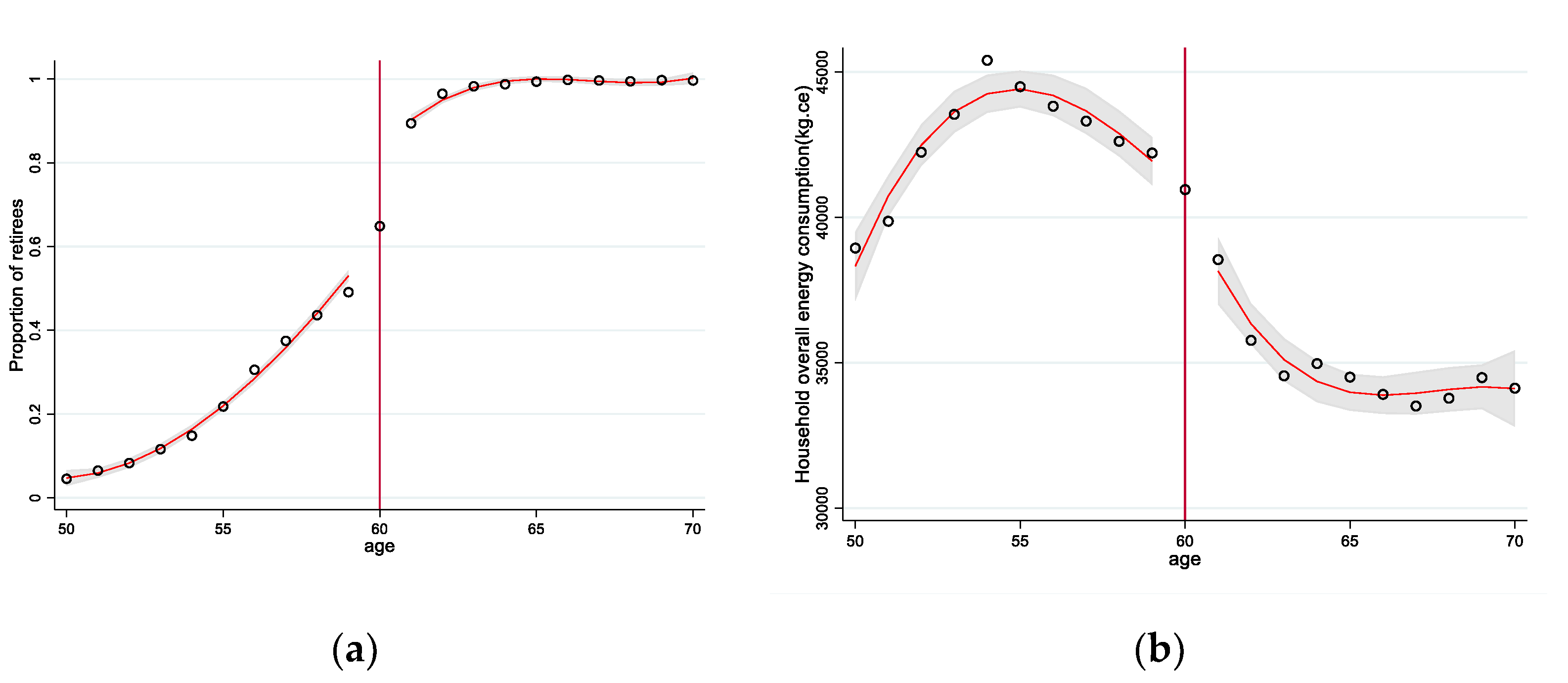
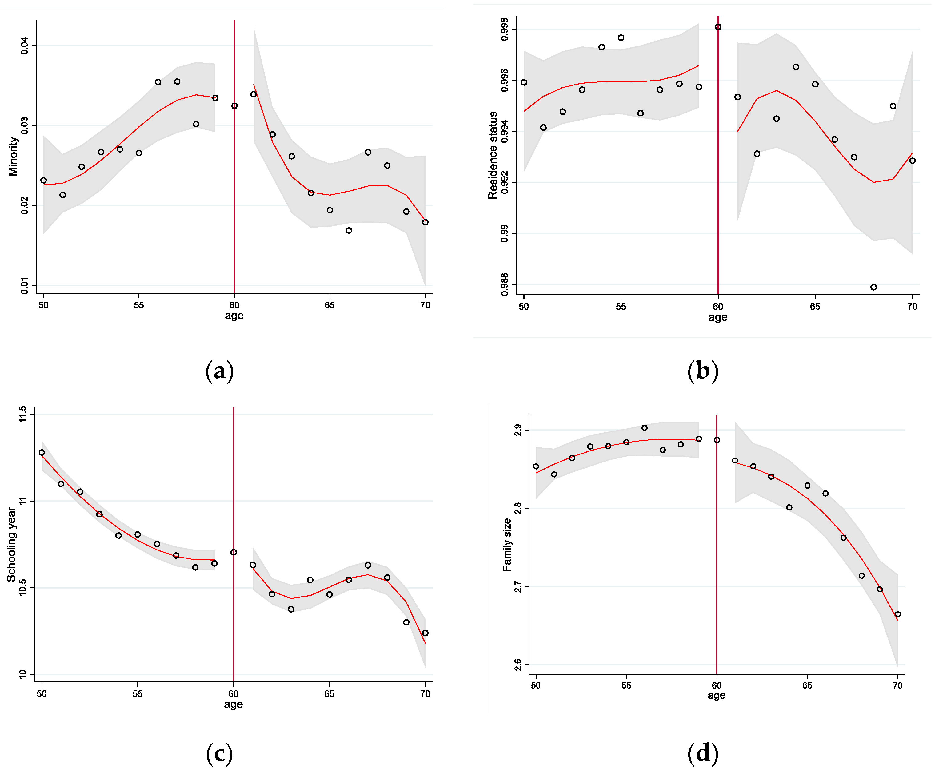
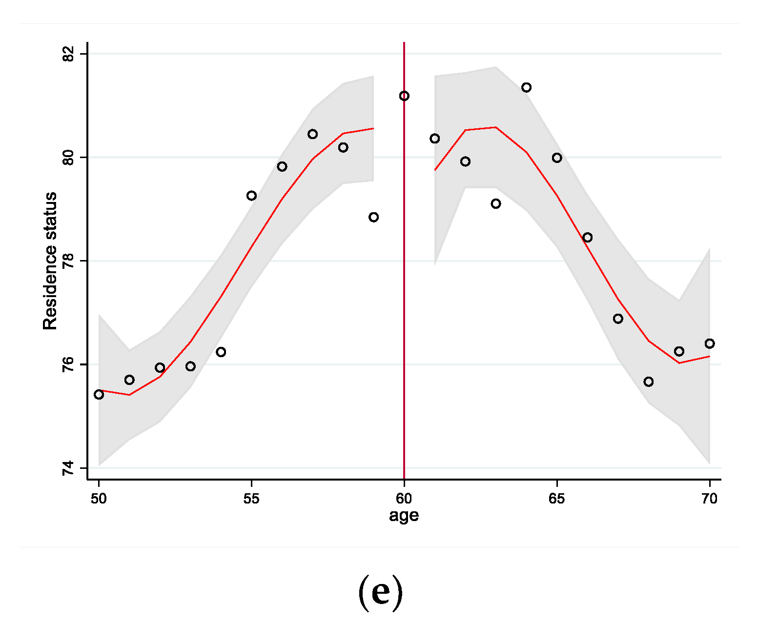
4.3. Validity of the RDD

An effective RDD requires that no other variables undergo a sharp change at the cutoff point. We then test the validity of our RDD, which is supported by both Figure 2 and the regression result of

Table 4. Results of validity of the RDD.

	Second Stage Results
Variables	Minority	Residence_Status	Schooling_Year	Housing_Area	Family_Size
Retired	−0.005	−0.001	0.036	−0.011	−1.187
(IV:Age > 60)	(0.008)	(0.003)	(0.128)	(0.053)	(1.794)
Constant	0.068 ***	1.003 ***	10.846 ***	3.027 ***	64.746 ***
	(0.007)	(0.002)	(0.122)	(0.039)	(1.678)
Observations	35,948	35,948	35,948	35,948	35,948
R-squared	0.025	0.003	0.029	0.026	0.093

Standard error is given in brackets. *** denotes significance levels of 1%. Source: author’s regression based on data from China’s Urban Household Survey.

. The variables we test include minority status, residence status, schooling year, family size and housing areas. We find there is no sharp change in those variables at the age 60 (Figure 2), which supports the pre-assumption of our RDD intuitively. We then confirm our findings using the regressions methodology, and the results are shown in Table 4, as the coefficient on “retired” is not significant for all five outcome variables, that is, the RDD of this study is valid.

4.4. Robustness Checks

Next, we conduct a series of robustness tests to confirm that the research results are robust.

4.4.1. Considering Wealth Level

Household energy consumption likely depends on the wealth level at retirement. We first investigate whether wealth affects the impacts of retirement on household energy consumption by using housing area as a wealth proxy. The results in

Table 5. Results of robustness checks: considering wealth level.

Variables	Housing Area in the Bottom 50 Percentile	Housing Area in the Top 50 Percentile
lnhousehold_energy	−0.023 (0.012) **	−0.037 (0.013) ***
lndirect	0.097 (0.015) ***	0.063 (0.016) ***
lnindirect	−0.081 (0.015) ***	−0.074 (0.016) ***
lnwork_relate	−0.611 (0.020) ***	−0.521 (0.021) ***
lnnon_work_relate	−0.000 (0.012)	−0.015 (0.013)
lnnon_durable	−0.148 (0.010) ***	−0.105 (0.011) ***
lndurable	0.057 (0.014) ***	0.011 (0.015)
lnhomefood	0.073 (0.008) ***	0.101 (0.009) ***
lnoutfood	−0.627 (0.027) ***	−0.502 (0.029) ***
lncigar	−0.399 (0.029) ***	−0.363 (0.030) ***
lnalcoh	−0.175 (0.020) ***	−0.204 (0.021) ***

Standard error is given in brackets. *** and ** denote significance levels of 1% and 5% respectively. Source: author’s regression based on data from China’s Urban Household Survey.

show that the impact of retirement on total household energy consumption is larger for those whose housing area is in the top 50 percentile compared to poor households (column 1, i.e., those having housing areas in the bottom 50th percentile). However, we derive similar results from both samples, showing that our results are robust and are not affected by household wealth level, although heterogenous marginal effects show up in terms of the components of total energy consumption.

4.4.2. Considering Female Head of Household

The next consideration is that in any urban household, either a man or a woman can be the head. Considering only the retirement age of male households may be biased, and the results may not be reliable. Therefore, we included the female household head in the sample in order to re-estimate the model. The regression results are shown in

Table 6. Results of robustness checks: considering female head of household.

	First-Stage Results	Second-Stage Results
Variables	Retired	Lnhouse_Energy	Lndirect	Lnindirect	Lnwork_Relate	Lnnon_Work_Relate
Age > 60	0.240 ***
	(0.018)
Retired		−0.021 **	0.093 ***	−0.067 ***	−0.622 ***	0.005
(IV:Age > 60)		(0.009)	(0.012)	(0.012)	(0.015)	(0.009)
Constant	0.685 ***	6.023 ***	4.632 ***	5.450 ***	2.569 ***	5.967 ***
	(0.015)	(0.057)	(0.079)	(0.068)	(0.089)	(0.058)
Observations	48,723	48,723	48,723	48,723	48,723	48,723
R-squared	0.426	0.202	0.125	0.183	0.243	0.189
F-value	415.09

Standard error is given in brackets. *** and** denote significance levels of 1% and 5% respectively. Source: author’s regression based on data from China’s Urban Household Survey.

. It can be seen that the regression coefficients are slightly different from those in Table 2, but they are consistent with the conclusions of the benchmark regression. As such, we believe that an analysis method that only considers husbands who work in formal sectors before retirement as the sample is robust.

4.4.3. Excluding 60-Year-Olds

In the previous analysis, we included households with husbands aged 60; however, the results of this sample may not be valid because of the mixture of pre- and post-retirement energy consumption. We thus now check whether the results remain robust if we drop households with husbands aged 60 (1571 observations in the previous sample). The results in

Table 7. Results of robustness checks: excluding 60-year-olds.

	First-Stage Results	Second-Stage Results
Variables	Retired	Lnhouse_Energy	Lndirect	Lnindirect	Lnwork_Relate	Lnnon_Work_Relate
Age > 60	0.296 ***
	(0.013)
Retired		−0.026 ***	0.078 ***	−0.071 ***	−0.553 ***	−0.004
(IV:Age > 60)		(0.009)	(0.011)	(0.011)	(0.014)	(0.009)
Constant	0.660 ***	6.019 ***	4.677 ***	5.437 ***	2.379 ***	5.968 ***
	(0.029)	(0.064)	(0.086)	(0.077)	(0.100)	(0.065)
Observations	34,377	34,377	34,377	34,377	34,377	34,377
R-squared	0.202	0.202	0.140	0.177	0.261	0.189
F-value	19.08

Standard error is given in brackets. *** denotes significance levels of 1%. Source: author’s regression based on data from China’s Urban Household Survey.

show that the regressions for the sample excluding 60-year-olds are indeed a little bit stronger, though overall consistent with previous findings.

4.4.4. Using Samples of Different Age Groups

The RDD identification relies on a sample around the age of 60. To determine the robustness of our main results, we finally use samples with different age ranges. The regressions are specified as being the same as those in Table 2, except that we use different samples. The results in

Table 8. Results of robustness checks: using samples of different age groups.

Variables	[55, 64]	[56, 63]	[57, 62]	[58, 62]
Retired	−0.069 ***	−0.062 ***	−0.084 ***	−0.090 **
(IV:Age > 60)	(0.019)	(0.023)	(0.029)	(0.042)
Constant	6.094 ***	6.022 ***	5.997 ***	5.919 ***
	(0.094)	(0.107)	(0.134)	(0.167)
Observations	15,919	12,584	9315	6172
R-squared	0.206	0.203	0.204	0.204

Standard error is given in brackets. *** and ** denote significance levels of 1% and 5% respectively. Source: author’s regression based on data from China’s Urban Household Survey.

show that the effect of retirement on household energy consumption is significant at the 1% level, and confirm our finding that the mandatory retirement policy does affect household energy consumption.

5. Conclusions

Against the backdrop of ever-increasing energy consumption, China is also facing the challenge of an aging population. Based on the urban household survey data from 2002 to 2009, this paper uses the exogenous impact of the retirement system on the retirement decision-making of male household heads in urban households, adopting a regression discontinuity design method to test the impact of the retirement of the male head of a household in Chinese urban households on the structure of household energy consumption, and to explore the reasons for this.

First, two-stage regression estimates find that, on the one hand, retirement significantly reduces the overall energy consumption of urban households by about 2.5%. Specifically, retirement greatly reduces household energy consumption expenditure related to work by about 55.4%, reduces non-durable products by about 12.1%, reduces dining out consumption by about 55.3%, and reduces energy consumption via tobacco and alcohol by 38.5% and 18.6%, respectively. On the other hand, although retirement induces a lower income, the energy consumed via durable products by the household increases, suggesting that our results confirm the consumption-smoothing hypothesis from the perspective of household energy consumption. The mechanism behind this is that a household reduces its social activities after retirement and its inhabitants spend much more time at home, such that the direct energy consumed increases and the indirect energy consumed decreases. The reduction in household non-durable energy consumption expenditure after retirement is closely related to the reduction in work-related energy consumption.

Secondly, the robustness tests find that variables that should not be affected by the retirement system are continuous around the breakpoint; after including female heads of households in the research, it is found that the regression coefficients of retirement on various energy consumptions are slightly different, but the sign and significance of the coefficients are not different in the estimation results that only consider the male heads of households. In addition, excluding the 60-year-old sample and using samples from different age groups did not significantly change the estimated coefficients, but the absolute value of the regression coefficients for samples with larger age groups would be larger; this means that as age increases, retirement has a stronger inhibitory effect on energy consumption. The results remain robust when considering household wealth levels, although a heterogenous marginal effect shows up in terms of the components of total energy consumption.

It should be noted that one limitation to this study is that, due to data constraints, the household energy consumption we calculated may suffer a bias based on the energy intensity of household expenditure, which may change endogenously, while we assumed the energy intensity of expenditure would no change. We believe that in future studies, the results may be more robust if more direct statistics and information on household energy consumption are used. In addition, the male household head samples in this paper are all from the formal sector (including government departments, public sectors, state-owned enterprises and institutions, etc.), which exhibits a better implementation of the retirement system. These workers have more stable income expectations and good pension insurance, as well as other benefits, and are less affected by the reform of the retirement system. Therefore, in further research, workers in the informal sector should be considered for analysis.

References

1. Pablo-Romero, M.D.P.; Pozo-Barajas, R.; Yñiguez, R. Global changes in residential energy consumption. Energ. Policy 2017, 101, 342–352. [Google Scholar] [CrossRef]
2. Creutzig, F.; Baiocchi, G.; Bierkandt, R.; Pichler, P.; Seto, K.C. Global typology of urban energy use and potentials for an urbanization mitigation wedge. Proc. Natl. Acad. Sci. USA 2015, 112, 6283–6288. [Google Scholar] [CrossRef] [PubMed]
3. Salari, M.; Kelly, I.; Doytch, N.; Javid, R.J. Economic growth and renewable and non-renewable energy consumption: Evidence from the U.S. states. Renew. Energ. 2021, 178, 50–65. [Google Scholar] [CrossRef]
4. Dhakal, S. Urban energy use and carbon emissions from cities in China and policy implications. Energ. Policy 2009, 37, 4208–4219. [Google Scholar] [CrossRef]
5. Lin, J.; Cao, B.; Cui, S.; Wang, W.; Bai, X. Evaluating the effectiveness of urban energy conservation and GHG mitigation measures: The case of Xiamen city, China. Energ. Policy 2010, 38, 5123–5132. [Google Scholar] [CrossRef]
6. Liang, S.; Zhang, T. Managing urban energy system: A case of Suzhou in China. Energ. Policy 2011, 39, 2910–2918. [Google Scholar] [CrossRef]
7. Madlener, R.; Sunak, Y. Impacts of urbanization on urban structures and energy demand: What can we learn for urban energy planning and urbanization management? Sustain. Cities Soc. 2011, 1, 45–53. [Google Scholar] [CrossRef]
8. Zhao, X.; Li, N.; Ma, C. Residential energy consumption in urban China: A decomposition analysis. Energ. Policy 2012, 41, 644–653. [Google Scholar] [CrossRef]
9. Cai, B.; Zhang, L. Urban CO2 emissions in China: Spatial boundary and performance comparison. Energ. Policy 2014, 66, 557–567. [Google Scholar] [CrossRef]
10. Zhou, N.; Fridley, D.; Khanna, N.Z.; Ke, J.; McNeil, M.; Levine, M. China’s energy and emissions outlook to 2050: Perspectives from bottom-up energy end-use model. Energ. Policy 2013, 53, 51–62. [Google Scholar] [CrossRef]
11. Mi, Z.; Meng, J.; Guan, D.; Shan, Y.; Song, M.; Wei, Y.; Liu, Z.; Hubacek, K. Chinese CO2 emission flows have reversed since the global financial crisis. Nat. Commun. 2017, 8, 1712. [Google Scholar] [CrossRef] [PubMed]
12. Meng, J.; Mi, Z.; Yang, H.; Shan, Y.; Guan, D.; Liu, J. The consumption-based black carbon emissions of China’s megacities. J. Clean Prod. 2017, 161, 1275–1282. [Google Scholar] [CrossRef]
13. Meng, J.; Liu, J.; Yi, K.; Yang, H.; Guan, D.; Liu, Z.; Zhang, J.; Ou, J.; Dorling, S.; Mi, Z.; et al. Origin and Radiative Forcing of Black Carbon Aerosol: Production and Consumption Perspectives. Environ. Sci. Technol. 2018, 52, 6380–6389. [Google Scholar] [CrossRef] [PubMed]
14. Wu, X.D.; Guo, J.L.; Ji, X.; Chen, G.Q. Energy use in world economy from household-consumption-based perspective. Energ. Policy 2019, 127, 287–298. [Google Scholar] [CrossRef]
15. Pachauri, S.; Jiang, L. The household energy transition in India and China. Energ. Policy 2008, 36, 4022–4035. [Google Scholar] [CrossRef]
16. Donglan, Z.; Dequn, Z.; Peng, Z. Driving forces of residential CO2 emissions in urban and rural China: An index decomposition analysis. Energ. Policy 2010, 38, 3377–3383. [Google Scholar] [CrossRef]
17. Feng, Z.; Zou, L.; Wei, Y. The impact of household consumption on energy use and CO2 emissions in China. Energy (Oxford) 2011, 36, 656–670. [Google Scholar] [CrossRef]
18. Biying, Y.; Zhang, J.; Fujiwara, A. Analysis of the residential location choice and household energy consumption behavior by incorporating multiple self-selection effects. Energ. Policy 2012, 46, 319–334. [Google Scholar] [CrossRef]
19. Golley, J.; Meng, X. Income inequality and carbon dioxide emissions: The case of Chinese urban households. Energ. Econ. 2012, 34, 1864–1872. [Google Scholar] [CrossRef]
20. Yu, B.; Zhang, J.; Fujiwara, A. Representing in-home and out-of-home energy consumption behavior in Beijing. Energ. Policy 2011, 39, 4168–4177. [Google Scholar] [CrossRef]
21. Yu, B.; Zhang, J.; Fujiwara, A. Evaluating the direct and indirect rebound effects in household energy consumption behavior: A case study of Beijing. Energ. Policy 2013, 57, 441–453. [Google Scholar] [CrossRef]
22. Thøgersen, J. Housing-related lifestyle and energy saving: A multi-level approach. Energ. Policy 2017, 102, 73–87. [Google Scholar] [CrossRef]
23. Hu, Z.; Wang, M.; Cheng, Z.; Yang, Z. Impact of marginal and intergenerational effects on carbon emissions from household energy consumption in China. J. Clean Prod. 2020, 273, 123022. [Google Scholar] [CrossRef]
24. Liu, M.; Huang, X.; Chen, Z.; Zhang, L.; Qin, Y.; Liu, L.; Zhang, S.; Zhang, M.; Lv, X.; Zhang, Y. The transmission mechanism of household lifestyle to energy consumption from the input-output subsystem perspective: China as an example. Ecol. Indic. 2021, 122, 107234. [Google Scholar] [CrossRef]
25. Zi, C.; Qian, M.; Baozhong, G. The consumption patterns and determining factors of rural household energy: A case study of Henan Province in China. Renew. Sustain. Energy Rev. 2021, 146, 111142. [Google Scholar] [CrossRef]
26. Belaïd, F.; Garcia, T. Understanding the spectrum of residential energy-saving behaviours: French evidence using disaggregated data. Energ. Econ. 2016, 57, 204–214. [Google Scholar] [CrossRef]
27. Belaïd, F. Understanding the spectrum of domestic energy consumption: Empirical evidence from France. Energ. Policy 2016, 92, 220–233. [Google Scholar] [CrossRef]
28. Belaïd, F. Untangling the complexity of the direct and indirect determinants of the residential energy consumption in France: Quantitative analysis using a structural equation modeling approach. Energ. Policy 2017, 110, 246–256. [Google Scholar] [CrossRef]
29. Feng, Q.; Yeung, W.J.; Wang, Z.; Zeng, Y. Age of Retirement and Human Capital in an Aging China, 2015–2050. Eur. J. Popul. 2019, 35, 29–62. [Google Scholar] [CrossRef]
30. United Nations. World Population Prospects: The 2015 Revision; United Nations Publications: New York, NY, USA, 2015. [Google Scholar]
31. Ota, T.; Kakinaka, M.; Kotani, K. Demographic effects on residential electricity and city gas consumption in the aging society of Japan. Energ. Policy 2018, 115, 503–513. [Google Scholar] [CrossRef] [Green Version]
32. Hamza, N.; Gilroy, R. The challenge to UK energy policy: An ageing population perspective on energy saving measures and consumption. Energ. Policy 2011, 39, 782–789. [Google Scholar] [CrossRef]
33. Liddle, B.; Lung, S. Age-structure, urbanization, and climate change in developed countries: Revisiting STIRPAT for disaggregated population and consumption-related environmental impacts. Popul. Environ. 2010, 31, 317–343. [Google Scholar] [CrossRef]
34. Kanaroglou, P.; Mercado, R.; Maoh, H.; Páez, A.; Scott, D.M.; Newbold, B. Simulation Framework for Analysis of Elderly Mobility Policies. Transp. Res. Rec. J. Transp. Res. Board 2008, 2078, 62–71. [Google Scholar] [CrossRef]
35. Okada, A. Is an increased elderly population related to decreased CO2 emissions from road transportation? Energ. Policy 2012, 45, 286–292. [Google Scholar] [CrossRef]
36. Yamasaki, E.; Tominaga, N. Evolution of an aging society and effect on residential energy demand. Energ. Policy 1997, 25, 903–912. [Google Scholar] [CrossRef]
37. Li, H.; Shi, X.; Wu, B. The retirement consumption puzzle revisited: Evidence from the mandatory retirement policy in China. J. Comp. Econ. 2016, 44, 623–637. [Google Scholar] [CrossRef]
38. Dong, Y.; Yang, D.T. Mandatory retirement and the consumption puzzle: Disentangling price and quantity declines. Econ. Inq. 2017, 55, 1738–1758. [Google Scholar] [CrossRef]
39. Bertogg, A.; Strauß, S.; Vandecasteele, L. Linked lives, linked retirement? Relative income differences within couples and gendered retirement decisions in Europe. Adv. Life Course Res. 2021, 47, 100380. [Google Scholar] [CrossRef]
40. Kuhn, U.; Grabka, M.M.; Suter, C. Early retirement as a privilege for the rich? A comparative analysis of Germany and Switzerland. Adv. Life Course Res. 2021, 47, 100392. [Google Scholar] [CrossRef]
41. Borozan, D. Unveiling the heterogeneous effect of energy taxes and income on residential energy consumption. Energ. Policy 2019, 129, 13–22. [Google Scholar] [CrossRef]
42. Giles, J.; Wang, D.; Cai, W. The Labor Supply and Retirement Behavior of China’s Older Workers and Elderly in Comparative Perspective; World Bank Policy Research Working Paper No. 5853; World Bank: Washington, DC, USA, 2011. [Google Scholar]
43. Iyer, L.; Meng, X.; Qian, N.; Zhao, X. Economic transition and private-sector labor: Evidence from urban China. J. Comp. Econ. 2019, 47, 579–600. [Google Scholar] [CrossRef]
44. Hahn, J.; Todd, P. Wilbert Identification and Estimation of Treatment Effects with a Regression-Discontinuity Design Source. Econom. Soc. 2001, 1, 201–209. [Google Scholar] [CrossRef]
45. Thistlewaite, D.L.; Campbell, D.T. Regression-Discontinuity Analysis: An Alternative to the Ex-Post Facto Experiment. J. Educ. Psychol. 1960, 2, 119–128. [Google Scholar] [CrossRef]
46. Imbens, G.W.; Lemieux, T. Regression discontinuity designs: A guide to practice. J. Econom. 2008, 142, 615–635. [Google Scholar] [CrossRef]
47. Dong, Y. Regression Discontinuity Applications with Rounding Errors in the Running Variable. J. Appl. Econ. 2015, 3, 422–446. [Google Scholar] [CrossRef]
48. Kolesar, M.; Rothe, C. Inference in Regression Discontinuity Designs with a Discrete Running Variable. Am. Econ. Rev. 2018, 108, 2277–2304. [Google Scholar] [CrossRef]
49. Wei, Y.; Liu, L.; Fan, Y.; Wu, G. The impact of lifestyle on energy use and CO2 emission: An empirical analysis of China’s residents. Energ. Policy 2007, 35, 247–257. [Google Scholar] [CrossRef]
50. Aguiar, M.; Hurst, E. Deconstructing Lifecycle Expenditure. In Proceedings of the 2008 Annual Meeting of the Society for Economic Dynamics, Cambridge, MA, USA, 10–12 July 2008; p. 771. [Google Scholar]
51. Zhang, H. The Hukou system’s constraints on migrant workers’ job mobility in Chinese cities. China Econ. Rev. 2010, 21, 51–64. [Google Scholar] [CrossRef]
52. Modigliani, F.; Brumberg, R. Utility analysis and the consumption function: An interpretation of cross-section data. Fr. Modigliani 1954, 1, 388–436. [Google Scholar]
53. Friedman, M. The permanent income hypothesis. In A Theory of the Consumption Function; Princeton University Press: Princeton, NJ, USA, 1957; pp. 20–37. [Google Scholar]
Figure 1. (a) Age and retirement rate; (b) age and energy consumption. Source: author’s drawing based on data from China’s Urban Household Survey.
Sustainability 14 12347 g001
Figure 2. Validity of the RDD. (a) age and minority; (b) age and residence status; (c) age and schooling year; (d) age and family size; (e) age and housing area. Source: author’s drawing based on data from China’s Urban Household Survey.
Sustainability 14 12347 g002aSustainability 14 12347 g002b