Abstract
How significantly and through what mechanisms can regional economic disparity be shaped by fiscal incentives? This paper uses the exemption of the agricultural tax in 2005 across China as a natural experiment to answer this question. Using a “difference-in-differences” model, which allows us to make within-group comparisons before and after the reform, we show that the revenue loss of county governments aggravated inter-regional economic disparity. Reasons behind it lie in the different tactics that local governments employed when dealing with the financial stress. In particular, governments in lower-income regions chose a negative way including tougher tax enforcement and less production-oriented investments, while those in higher-income localities embraced positive taxation and expenditure strategies to attract more capital inflow. This paper helps shed light on how to optimize fiscal system arrangement to alleviate the broadening regional economic disparity and improve local fiscal sustainability.
1. Introduction
Fiscal decentralization has been one of the most common arrangements in dealing with the intergovernmental relations, especially in the developing world. It is well acknowledged that fiscal delegation from central to local governments allows the latter to acquire a larger proportion of local revenue, thus incentivizing local public goods provision and economic growth [1,2,3,4]. However, in addition to their achievements, developing countries are also involved in unsustainable and inadequate development. There is growing attention on how to value or promote balanced and sustainable growth for developing countries. Take public health outcomes as an example. Studies find that although past decades have witnessed emerging economies, typically non-OECD countries, such as China, India, Brazil and other ASEAN or BRICS members’ highly successful economic reforms, their public health development is still on a struggling track to alleviate the remarkable domestic heterogeneity [5,6,7]. Just like healthcare performance, other development outcomes, such as business and educational goods provision, are largely dependent on the government’s efficiency, for it not only needs the government to raise revenue from the public but also to organize the investment [8]. Some scholars have attributed this unsustainable growth problem to various policy choices of local governments under specific fiscal incentives [9,10,11,12]. However, most existing literature has noticed the relationship between fiscal decentralization and local economic performance, but few have rigorously explored the role of fiscal incentives in determining the policy choices of local governments.
China provides an ideal context to explore this fiscal incentive conjecture. Fiscal decentralization has been recognized as one of the most important institutional factors in driving its rapid economic growth, especially since the late 1990s (see a review article by Xu (2011) [13]). Fiscal decentralization is often referred to as “federalism, Chinese style” because the Tax Sharing System Reform launched in 1994 fundamentally changed the dynamics of how central and local governments divide tax revenue [14]. On the one hand, it transferred revenue from local governments to the center but failed to adjust expenditure responsibilities for local governments on the other. As a result, there is a mismatch between local governments’ revenue and expenditure, which leads to greater reliance on intergovernmental fiscal transfers, but this still could not help fill the local fiscal revenue and expenditure gap [15,16]. As shown in Figure 1, there is a significant drop in the proportion of local budgetary revenue to total revenue after 1994. It seems reasonable to derive a corollary that local officials take an inactive attitude when facing this combination of heavy expenditure responsibilities and tightening financial budgets.
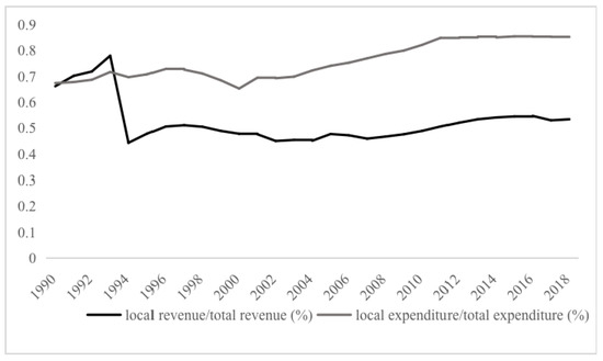
Figure 1.
Subnational budgetary revenue and expenditure in China. Source: China Statistical Yearbook (1989–2019).
Actually, at the same time, the political centralization system enables the central government to generate “tournament-like” political incentives to solve this dilemma. In particular, it uses promotions and punishments to motivate local officials to adopt pro-business policies that focus on the economic growth in their jurisdictions [17,18,19,20,21].
Given the fact that Chinese counties exhibit quite different economic performances, it is straightforward that the same institutional arrangement brings about different types of incentives to different local governments. A major challenge in identifying the responses of local governments to the changing fiscal revenue incentives is that fiscal revenue is endogenous, as a number of confounders may simultaneously affect the outcome variables and local governments’ behaviors.
To answer this question, this paper exploits the exemption of the agricultural tax in China in 2005 as an exogenous “fiscal pressure” shock in which county governments experienced a severe revenue loss. Under this unexpected financial stress, local governments tend to act in different ways to reconcile the dilemma of extracting fiscal revenue and facilitate local economic growth. Using the county-level variations in revenue loss allows us to apply a standard “difference-in-differences” approach to identify the causal effects of fiscal pressure on policy choices of local governments in China.
Our paper finds that negative revenue shock indeed widened the disparity of regional economic development. We further explore the mechanisms behind it. The results show that governments with various initial economic endowments tended to act in different ways when dealing with fiscal stress. In particular, governments in low-income regions chose a negative way, including more strict tax enforcement and less production-oriented investments, while high-income regions embraced positive taxation and expenditure strategies to attract more capital inflow. Being trapped in this vicious circle is one of the reasons that low-income regions have been left far behind the high-income ones as time goes by.
The rest of the paper proceeds as follows. Section 2 reviews the literature. Section 3 introduces the institutional background. Section 4 describes data sources. Section 5 introduces the Abolition of Chinese Agricultural Tax Reform as a quasi-natural experiment and discusses the empirical strategy. Section 6 presents the empirical results. Section 7 concludes.
2. Literature Review
The economics literature has shown a growing interest in fiscal decentralization as a driving force of economic growth in developing countries [22,23,24]. Since there is no consensus on whether a fiscal decentralization arrangement plays a helping or grabbing hand in regional economic development, a strand of literature attributes it to local governments, which our paper also mainly speaks to.
Our study contributes to the existing literature in the following ways. First, we document more facts on fiscal incentives and development in developing countries [12,25,26,27]. Studies on a few developing countries suggest that economic growth tends to be faster, where local governments can acquire higher sharing rates of revenue generated in their own jurisdiction [14]. A case in Russia suggests that the lack of fiscal incentives can partly explain why local governments act like predators towards private firms [28]. This fiscal incentive explanation is also in line with findings in other developing countries such as Mexico [29]. Compared to this strand of work, our paper especially focuses on regional economic disparity by providing more evidence on how local governments with different initial economic conditions respond to fiscal incentives caused by local fiscal distress. We find that in addition to what previous literature has argued about the role of fiscal incentives in shaping local economic growth patterns, heterogeneous effects may appear, even given the same fiscal incentive.
Second, the findings of our paper also add to the fiscal decentralization literature. Studies show that the roles played by the government system in the developing economies under fiscal decentralization all face the important agency problem between the central and local governments [18,30,31]. We also provide new evidence to the existing literature; specifically, we find that under the economic competition among local governments, the abrupt revenue-loss shock lead to short-termist behaviors in lower-income regions and aggravated economic growth, which goes against the original intention of the policy. This paper examines the sole effect of revenue centralization and shows its heterogeneous effects on local economic development. In this way, our paper helps explain a series of challenges that confront the developing economies.
Lastly, the results shed light on how to optimize the fiscal system design to balance the efficiency and sustainability of economic development to other developing countries [32]. There is limited research focusing on developing countries in the strand of literature studying the effect of fiscal system arrangement on regional disparity. However, just as Cont et al. (2017) [33] point out, in developing countries such as Argentina, the redistributive and stabilizing functions of the fiscal and tax systems have little impact due to the inefficient fiscal system arrangement. Studies in terms of taxation in developing strategies also reveals the side-effects of inappropriate fiscal system design. Mudiyanselage et al. (2020) [34] investigate the problem of the declining tax to GDP ratio in Sri Lanka by estimating the tax efforts of lower-middle-income countries. They find that weak tax enforcement are major challenges for developing countries to achieve sustained growth, due to the lack of fiscal incentives and ubiquitous rent-seeking opportunities. Our paper linked to this strand of work by providing evidence on how lower-income regions arrange their fiscal activities. One lesson that can be drawn is that developing countries should pay more attention to sharing information between different regulatory authorities and also conducting monitoring and consulting from the upper levels of government.
3. China’s Fiscal System and Local Government Behavior
Fiscal revenues are distributed top-down along the administrative hierarchy in China: the central, provincial, prefectural, county and township governments. Actually, county governments are the last to enjoy the de facto power to make development blueprints [35]. China’s fiscal system has experienced three large rounds of reform, both of them concentrated on the revenue-sharing arrangement. The 1994 reform of the tax sharing system allowed the central government to share 75% of the value-added tax, the 2002 tax reform further allowed the central government to take 60% of the corporate income tax. The abolition of agricultural tax reform in 2005 made it even worse for the county governments since this tax is one of the important revenue sources for them. Those reforms collectively add fiscal burdens to local governments.
This fiscal contracting scheme has incentivized local governments to take different actions to maximize revenues for decades [25]. To better capture the logic behind fiscal incentives on local government behavior, we first characterize total fiscal revenue in the following equation:
where is the statuary sharing ratio of fiscal revenue between local governments and the upper-level governments (Because we focus on the county-level government, the upper-level governments here includes the prefectural, the provincial and the central government); is the effective tax rate and B is the size of tax base. Local governments then have the following three ways to maximize their total fiscal revenue.
First, local governments can directly influence the effective tax rate through tax enforcement [36] and tax break policies [37,38]. Although statutory tax rates do exist, there is still room for local governments to use tax-related policies as instruments in attracting investments. Chen (2017) [36] points out revenue loss on county governments in China can be largely and quickly offset by tougher tax enforcement, which imposes a greater effective tax rate. However, Chen and Zhang (2021) [38] show that local officials are likely to leverage tax break policies, a tool for increasing investment and expanding economic activities. Indeed, Chen et al. (2021) [39] document the fact that the effective corporate income tax rate deviates considerably from the statutory rate, as a bunch of tax cut policies induce this dispersion.
Second, local governments can acquire fiscal revenue using policy tools from a expenditure side, which helps expand the tax base B. This policy box contains more production-oriented fiscal expenditure, such as investments on roads, electricity, water supply and industrial parks, which in turn attracts more manufacturing firms to move in, leading to a sustained growth [40,41].
The last choice is extraction from the fees and levies such as reliance on land conveyance fee and informal fees to meet the shortfall of formal tax revenue [12,42,43], while this excessive reliance on land financing and collection of informal taxes may distort firm production.
The policy choices to maximize total revenue discussed above can therefore be classified into two large categories, one set of strategies is regarding taxation tactics including more tax-preferential policies and tougher tax enforcement and inspection; another set is targeted on the tax base, which includes industrial-oriented expenditure and levies extraction. We later show that policy choices have intimate relationships with the heterogeneity of local governments.
4. Data
This paper employs three datasets: (1) the Annual Survey of Industrial Production (ASIP) conducted by the National Bureau of Statistics of China (2001–2010); (2) the County Public Finance Statistics Yearbook of China (2001–2010); and (3) the China Statistical Yearbook of Regional Economy (2001–2014).
The ASIP is administered by the National Bureau of Statistics of China. It covers all state-owned enterprises (SOEs), as well as large and medium-sized non-SOEs with annual sales no less than RMB 5 million (approximately USD 800,000). Information for each firm is recorded, including its location, industry code, county-level region code, liability, assets, sales income, ownership, and tax payments, including value-added tax and corporate income tax. The ASIP is also based on direct investigation, avoiding possible manipulation or misreporting by local officials [44].
The County Public Finance Statistics Yearbook of China includes detailed government revenue and government expenditure at county and prefecture levels. We mainly use the following variables: (1) total revenue; (2) tax revenue; (3) total expenditure; (4) agricultural taxation revenue; (5) subsidies for agricultural taxation reform; (5) infrastructure expenditure; (6) agricultural expenditure; (7) education expenditure; (8) transfer from upper governments; and (9) land conveyance fee.
The China Statistical Yearbook of Regional Economy provides variables of time-varying characteristics of counties. We select (1) GDP, (2) total population, and (3) capital stock to capture the potential influences caused by these socioeconomic factors.
5. Empirical Strategy
5.1. China’s Exemption of Agricultural Tax in 2005
The abolition of agricultural tax is one of the policies implemented by the central government to alleviate the burdens for Chinese farmers. Before this exemption, agricultural tax accounts for about 5.6% of county governments’ total revenue and around 12% of the county governments’ tax revenue [36]. Despite the fact that a few counties had been chosen to carry out pilot reforms before 2005, it was the year 2005 that the nationwide abolition of agricultural taxes was enacted according to the official records. In order to support local governments in pushing forward this reform , the Ministry of Finance published an official document in which the upper governments were required to offer transfer payments to make up the potential revenue loss of county governments, but it was still far from enough (see the official document for details: http://www.gov.cn/zhengce/content/2008-03/28/content_2016.htm, retrieved on 19 February 2022).
Considering both the revenue loss and transfer subsidies due to the abolition of agricultural tax, we follow the practice of Chen (2017) [36] to measure the net revenue loss as follows:
where is the average agricultural tax income in county c between year 2001 and year 2004; and are the average agricultural transfer subsidized by upper governments before and after the abolition, respectively; while and are the total budgetary tax revenue with the same time range mentioned before. One thing worth noting is that analyzing the effect of the 2005 abolition of agricultural tax is not our ultimate goal. Instead, we merely use this reform as a quasi-experiment to discover the impacts of negative fiscal pressure on the later development performances.
5.2. Identification Strategy
To investigate the impact of the reform on inter-regional economic disparity and the policy choices of local governments, we basically conduct the following “difference-in-differences” specification:
where subscripts denote county, prefecture, and year, respectively. The dependent variable is the outcome variables, including logarithm value of GDP per capita, the growth rate of GDP per capita and policy choice outcomes of county governments later discussed at length in Section 6.2. is a dummy variable which equals 0 in the pre-reform period and 1 in the post-reform period. is the revenue loss to county c before the reform as measured by Equation (2). is a set of control variables including GDP per capita (log), Capital stock per capita (log), land conveyance fee (log) and intergovernmental transfer (log). We include prefecture-year () and county fixed effects () to account for prefecture-year and county time-invariant characteristics. Adding these fixed effects also allows us to make within-prefecture comparisons. is the key parameter of our interest as it captures the effect of the intensity of agricultural tax revenue loss. We relax the assumption of independent and identical distribution of error terms by clustering error terms at the prefecture level. That is, the correlation of error terms exists among counties in a given prefecture.
We present the summary statistics in Table 1.

Table 1.
Summary Statistics.
6. Empirical Results
6.1. Fiscal Pressure and Regional Economic Disparity
Before stepping into the quantified results, we first document a fact on Chinese county economic growth convergence. In the literature of growth economics, there are two types of convergence [45,46]: and . The former occurs when the dispersion of real income per capita across a group of economies falls over time while the latter occurs when the partial correlation between growth in income and its initial level over time is negative.
Figure 2 exhibits the of counties in China, where the dispersion of real income per capita is calculated based on the following population weighted coefficient of variation :
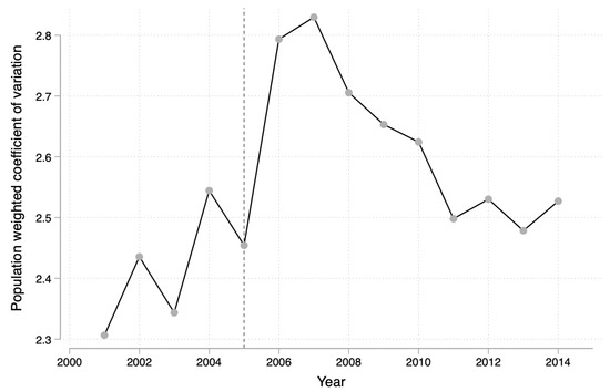
Figure 2.
Dynamic of Chinese counties. Source: China Statistical Yearbook of Regional Economy.
In Equation (4), subscripts i and t denote county and year, respectively, is the nationwide average of real GDP in year t and is the total population in year t. By definition, occurs as . Two pieces of information can be extracted from Figure 2. First, China did not experience a process of in general, especially before 2008. The dispersion of economic growth calculated by the population-weighted coefficient of variation inequality almost kept rising up before 2008 and after 2011. Second, the year 2005, which was the year that agricultural tax was officially exempted, witnessed a significant jump in the dispersion of income per capita. The unexpected loss of revenue impoverished county governments and brought about a bumped rise in regional economic disparity.
To empirically test the effects of fiscal pressure on regional economic disparity, we introduce one-year lagged value of GPD per capita () as an interaction term to model (3). Backed up by Barrow and Sala-i-Martin(1992) [45], we rewrite model (3) as Equation (5). What Barro’s convergence theory tells us is that convergence takes place when economic growth is negatively correlated with its initial level when exogenous variables remain constant. Under this setting, is now the coefficient of interest which captures the causal effect of revenue loss on county c’s economic growth conditioned on its economic performance in the past. When is positive, it means the fiscal pressure shock boosts economic growth when a county enjoyed better economic growth conditions before.
We report the results in Table 2. The dependent variable in column (1) and (3) is the logarithm value of GDP per capita, while in column (2) and (4), it is changed to the growth rate of GDP per capita for robustness check. Additionally, we exploit the one period lag of GDP per capita to measure the growth conditions benefited from the past in column (1) and (2), while in column (3) and (4), it is replaced by two periods’ lagged values for robustness checks. The significant and positive coefficients of in all the columns collectively show that the fiscal pressure shock makes high-income counties grow better but leaves the low-income counties in a deteriorated situation.
Table 2.
Robustness check.
We also conduct a robustness check based on a different method to divide the sample counties into “treatment group” and “control group”. In Table 2, we replace the continuous treatment variable into a dichotomous one. Specifically, we assign 1 to this new if the revenue loss is above the median and 0 if it is below it. This time, we can compare the difference of regional economic growth between the control group and the treatment group before and after the reform. Results under this new treatment assignment are still robust. Fiscal pressure did not cause a relative but a regional economic growth divergence instead.
6.2. Mechanism: Fiscal Pressure and Policy Choices of County Governments
Given the findings on fiscal pressure exacerbates regional economic disparity, in this section, we discuss how local governments react to this unexpected revenue loss. More specifically, we want to find out why this negative fiscal revenue shock widened the gap in economic growth between higher- and lower-income counties. Recall that, in Section 3, we argue that fiscal incentives help shape local governments’ policy choices mainly from taxation and expenditure sides.
We now test the reactions of governments in lower-income regions and governments in higher-income regions on fiscal revenue loss in terms of taxation strategies. To do so, we first divide the sample counties into two subgroups—a low-income one and a high-income one—by calculating the median value of GDP per capita. Counties with GDP per capita below the sample median are divided into a low-income subgroup while the remains belong to a high-income subgroup.
We estimate model (3) and report the results in Table 3. Here, the outcome variables are concerned with the tax burdens of local industrial firms which are one of the largest tax base for county governments. More importantly, it would in turn bring in service industries to further generate substantial business taxes. We use detailed tax-payable information from ASIP to generate variables and . The former denotes the average effective value-added tax rate of industrial firms in county c at year t, and the latter is the average effective income tax rate of industrial firms in county c at year t. Using this aggregate data instead of micro-data allows us to alleviate the effects caused by firm’s entry and exit. Columns (1) and (2) show the results when firms’ average effective value-added tax is a dependent variable, while in columns (3) and (4), firms’ average effective income tax burden serves as a dependent variable. Sample counties used in columns (1) and (3) are defined as low-income ones, while counties in columns (2) and (4) are high-income ones.
Table 3.
Fiscal Pressure and policy choices: taxation strategy.
The regression results show that no matter which indicator is chosen to proxy local governments’ policy choices of taxation strategy, firms’ value-added tax burdens and income tax burdens in the low-income regions have increased significantly after the agricultural tax reform as the coefficients of the interaction term are significantly positive at the 10% and 5% confidence levels. Although the value-added tax is collected by the State Taxation Administration independently, local governments still have the discretion to intervene in its collection. Things change when it comes to counties with higher income. is significant and negative in both column (2) and (4), which suggests that industrial firms located in these regions enjoy significantly lower tax burdens with confidence levels of 5% and 10% after the revenue loss shock.
All these findings collectively show how differently taxation policies are used when faced with negative revenue shock. In less-developed counties, firms face higher total burdens of value added tax and income tax, which is the result of tougher tax enforcement (tougher tax enforcement includes cracking down tax evasions and less preferential tax cut policies, etc.) employed by local governments. Instead of doing this, governments in high-income counties choose to continuously offer generous tax-preferential polices to attract an inflow of industrial investments. Our findings enrich what Chen (2017) [36] argues on fiscal pressure and tax enforcement to some extent.
We next explore how negative fiscal revenue shocks incentivize local governments to invest in public sectors. As the agent of the central government, local governments bear the responsibility of providing infrastructure to promote industrialization and urbanization and other public goods (such as healthcare, education and social security) to broader interests. The multi-functioning of county governments can be reflected in three indicators: investments in industrial infrastructure, agricultural expenditure and educational public goods. We then re-estimate model (3) using those indicators as outcome variables and report the results in Table 4.
Table 4.
Fiscal pressure and policy choices: expenditure strategy.
The positive and significant coefficients of in column (2) of Table 4 suggest that compared with governments in low-income counties, the revenue loss triggered a proactive attitude in infrastructure investments in counties with high income. It is worth noticing that in terms of educational public goods provision, both low-income counties and high-income counties tend to shrink their expenditure. Reasons behind this lie in the difficulty in using the quality of education provision as a criterion for officials’ performance evaluation. However, the large scale of infrastructure building can help attract firms’ entry and business contracts, which are all marked as a politician’s great achievements. It is also coordinated with a strand of literature discussing how Chinese decentralization caused a biased fiscal expenditure structure with emphasis on production rather than public needs [47,48]. Columns (5) and (6) report the performance of agriculture support. The positive and significant coefficients of the interaction term show that governments in low-income counties continued to rely on returns of agriculture after the fiscal pressure shock. Since agriculture has lower value-added than industries such as manufacturing and mining, counties with lower income may further be left behind in the future.
The discussions above collectively illustrate the strategies employed by county governments with different income levels when faced with a fiscal pressure shock. It shows that local governments in lower-income counties sustain lower rewarded tactics, including tougher tax enforcement and reliance on agricultural output. Governments in high-income counties tend to offer preferential and generous policies to attract capital inflow, which can be rewarded by future income.
7. Conclusions
Fiscal decentralization has important consequences on how political actors govern locally. Using China as an example, the exemption of agricultural taxes helps provide an exogenous policy change in fiscal revenue loss to conduct this empirical test. By drawing on data sets of Chinese county governments’ expenditure and income and information of industrial firms, we test the effects of the bursting fiscal stress on inter-regional economic disparity and the mechanisms of policy choices using a “difference-in-differences” model.
In summary, we find that abrupt revenue losses of county governments aggravated inter-regional economic disparity. More importantly, we show that in response to this fiscal pressure, county governments with different income levels tend to have different tactics to deal with this dilemma. In particular, governments in low-income regions choose a negative method, including tougher tax enforcement and less production-oriented investments, while those in high-income localities embrace positive taxation and expenditure strategies to provide more infrastructure to attract more capital inflow. The less-developed counties put emphasis on how to make up for the current revenue loss while developed counties try to deal with it by breeding future income. It is the difference in choosing how to deal with fiscal stress that can partly explain the deteriorating regional economic inequality.
Our research helps shed light on how fiscal arrangements incentivize local agents in a decentralized developing country. It has meaningful policy implications in terms of achieving a sustainable growth. One lesson that can be drawn from this paper is that policies should be made after considering the initial conditions of different regions. It is possible that less-developed regions would be short-sighted due to their limits in governance experience and official quality. The misuse of administrative power may harm the fiscal sustainability and, of course, the sustainability of economic growth. Our study also calls for attention on matters of cost-effective allocation of limited resources as the rising developing economies such as BRICS countries are mostly experiencing higher growth momentum with large consumption of natural and financial resources [7]. Therefore, how to incentivize local governments to do the right things is of great significance. Our paper suggests that things may be better off if more investments were made in advanced communication and information technology to facilitate monitoring and consulting, thus increasing the connectivity among government agencies. In addition, the legal department should be strengthened by limiting local officials’ discretionary power. There are still many issues that this paper does not cover. Specifically, we mainly test the fiscal incentives provided by abrupt revenue loss, but what about a positive revenue shock? In addition, what we focus on in this paper is a relatively short-run performance; what about the long-run effects? We leave these questions for future research.
Author Contributions
Conceptualization, X.Z. and M.R.; methodology, X.Z.; software, X.Z. and M.R.; validation, X.Z. and M.R.; writing—original draft preparation, X.Z.; writing—review and editing, M.R. All authors have read and agreed to the published version of the manuscript.
Funding
This research received no external funding.
Institutional Review Board Statement
Not applicable.
Informed Consent Statement
Not applicable.
Data Availability Statement
Please contact corresponding author.
Conflicts of Interest
The authors declare no conflict of interest.
References
- Tiebout, C.M. A Pure Theory of Local Expenditures. J. Political Econ. 1956, 64, 416–424. [Google Scholar] [CrossRef]
- Musgrave, R.A. The Theory of Public Finance: A Study in Public Economy; McGraw Hill: New York, NY, USA, 1959. [Google Scholar]
- Oates, W.E. An Essay on Fiscal Federalism. J. Econ. Lit. 1999, 37, 1120–1149. [Google Scholar] [CrossRef]
- Qian, Y.; Weingast, B.R. Federalism as a Commitment to Reserving Market Incentives. J. Econ. Perspects 1997, 11, 83–92. [Google Scholar] [CrossRef]
- Jakovljevic, M.; Sugahara, T.; Timofeyev, Y.; Rancic, N. Predictors of (in) Efficiencies of Healthcare Expenditure among the Leading Asian Economies–Comparison of OECD and Non-OECD Nations. Risk Manag. Healthc. Policy 2020, 13, 2261. [Google Scholar] [CrossRef] [PubMed]
- Jakovljevic, M.; Timofeyev, Y.; Ekkert, N.V.; Fedorova, J.V.; Skvirskaya, G.; Bolevich, S.; Reshetnikov, V.A. The impact of health expenditures on public health in BRICS nations. J. Sport Health Sci. 2019, 8, 516. [Google Scholar] [CrossRef] [PubMed]
- Jakovljevic, M.; Lamnisos, D.; Westerman, R.; Chattu, V.K.; Cerda, A. Future health spending forecast in leading emerging BRICS markets in 2030: Health policy implications. Health Res. Policy Syst. 2022, 20, 1–14. [Google Scholar]
- Angela, Y.C.; Krycia, C.; Angela, E.M.; Abigail, C.; Catherine, S.C.; Gloria, I.; Nafis, S.; Golsum, T.; Junjie, W.; Theodore, Y.; et al. Past, Present, and Future of Global Health Financing: A Review of Development Assistance, Government, Out-of-pocket, and other Private Spending on Health for 195 Countries, 1995–2050. Lancet 2019, 393, 2233–2260. [Google Scholar]
- Rodden, J. Reviving Leviathan: Fiscal Federalism and the Growth of Government. Int. Organ. 2003, 57, 695–729. [Google Scholar] [CrossRef]
- Weingast, B.R. Second Generation Fiscal Federalism: The Implications of Fiscal Incentives. J. Urban Econ. 2009, 65, 279–293. [Google Scholar] [CrossRef]
- Careaga, M.; Weingast, B.R. Fiscal Federalism, Good Governance, and Economic Growth in Mexico. In Search of Prosperity: Analytic Narratives on Economic Growth; Rodrik, D., Ed.; Book Section 13; Princeton University Press: Princeton, NJ, USA, 2012; pp. 399–436. [Google Scholar]
- Han, L.; Kung, J.K.S. Fiscal Incentives and Policy Choices of Local Governments: Evidence from China. J. Dev. Econ. 2015, 116, 89–104. [Google Scholar] [CrossRef]
- Xu, C. The Fundamental Institutions of China’s Reforms and Development. J. Econ. Lit. 2011, 49, 1076–1151. [Google Scholar] [CrossRef]
- Jin, H.; Qian, Y.; Weingast, B.R. Regional Decentralization and Fiscal Incentives: Federalism, Chinese Style. J. Public Econ. 2005, 89, 1719–1742. [Google Scholar] [CrossRef]
- Wong, C.P.W. Financing Local Government in the People’s Republic of China; Oxford University Press: Hongkong, China, 1997. [Google Scholar]
- Whiting, S.H. Fiscal Reform and Land Public Finance: Zouping County in National Context. In China’s Local Public Finance in Transition; Man, J., Hong, Y.H., Eds.; Lincoln Institute of Land Policy: Cambridge, MA, USA, 2010; pp. 125–144. [Google Scholar]
- Qian, Y.; Xu, C. The M-form Hierarchy and China’s Economic Reform. Eur. Econ. Rev. 1993, 37, 541–548. [Google Scholar] [CrossRef]
- Maskin, E.; Qian, Y.; Xu, C. Incentives, Information, and Organizational Form. Rev. Econ. Stud. 2000, 67, 359–378. [Google Scholar] [CrossRef]
- Blanchard, O.; Shleifer, A. Federalism with and without Political Centralization: China Versus Russia. IMF Staff. Pap. 2001, 48, 171–179. [Google Scholar]
- Li, H.; Zhou, L.A. Political Turnover and Economic Performance: The Incentive role of Personnel Control in China. J. Public Econ. 2005, 89, 1743–1762. [Google Scholar] [CrossRef]
- Enikolopov, R.; Zhuravskaya, E. Decentralization and Political Institutions. J. Public Econ. 2007, 91, 2261–2290. [Google Scholar] [CrossRef]
- Akai, N.; Sakata, M. Fiscal Decentralization Contributes to Economic Growth: Evidence from State-level Cross-section Data for the United States. J. Urban Econ. 2002, 52, 93–108. [Google Scholar] [CrossRef]
- Iimi, A. Decentralization and Economic Growth Revisited: An Empirical Note. J. Urban Econ. 2005, 57, 449–461. [Google Scholar] [CrossRef]
- Thornton, J. Fiscal Decentralization and Economic Growth Reconsidered. J. Urban Econ. 2007, 61, 64–70. [Google Scholar] [CrossRef]
- Gordon, R.H.; Li, W. Provincial and Local Governments in China: Fiscal Institutions and Government Behavior. In Capitalizing China; Book Section 8; University of Chicago Press: Chicago, IL, USA, 2012; pp. 337–369. [Google Scholar]
- Besley, T.; Burgess, R. The Political Economy of Government Responsiveness: Theory and Evidence from India. Q. J. Econ. 2002, 117, 1415–1451. [Google Scholar] [CrossRef]
- Besley, T.; Persson, T. Why Do Developing Countries Tax So Little? J. Econ. Perspect. 2014, 28, 99–120. [Google Scholar] [CrossRef]
- Zhuravskaya, E.V. Incentives to Provide Local Public Goods: Fiscal Federalism, Russian Style. J. Public Econ. 2000, 76, 337–368. [Google Scholar] [CrossRef]
- Smart, M. Taxation and Deadweight Loss in a System of Intergovernmental Transfers. Can. J. Econ. 1998, 31, 189–206. [Google Scholar] [CrossRef]
- Song, Z.; Storesletten, K.; Zilibotti, F. Growing Like China. Am. Econ. Rev. 2011, 101, 196–233. [Google Scholar] [CrossRef]
- Xiong, W. The Mandarin Model of Growth; Report; National Bureau of Economic Research: Cambridge, MA, USA, 2018. [Google Scholar]
- Gadenne, L.; Singhal, M. Decentralization in Developing Economies. Annu. Rev. Econ. 2014, 6, 581–604. [Google Scholar] [CrossRef]
- Cont, W.; Porto, A.; Juarros, P. Regional Income Redistribution and Risk-sharing: Lessons from Argentina. J. Appl. Econ. 2017, 20, 241–269. [Google Scholar] [CrossRef]
- Mudiyanselage, H.K.; Rammohan, A.; Chen, S.X. Tax Effort in Developing Countries: Where is Sri Lanka? J. Tax Adm. 2020, 6, 162–189. [Google Scholar]
- Cheung, S. The Economic System of China; CITIC Press: Beijing, China, 2009; Volume 10. [Google Scholar]
- Chen, S.X. The Effect of a Fiscal Squeeze on Tax Enforcement: Evidence from a Natural Experiment in China. J. Public Econ. 2017, 147, 62–76. [Google Scholar] [CrossRef]
- Liu, Y.; Tai, H.; Yang, C. Fiscal Incentives and Local Tax Competition: Evidence from China. World Econ. 2020, 43, 3340–3356. [Google Scholar] [CrossRef]
- Chen, L.; Zhang, H. Strategic Authoritarianism: The Political Cycles and Selectivity of China’s Tax-Break Policy. Am. J. Political Sci. 2021, 65, 845–861. [Google Scholar] [CrossRef]
- Chen, Z.; He, Y.; Liu, Z.; Serrato, J.C.S.; Xu, D.Y. The Structure of Business Taxation in China. Tax Policy Econ. 2021, 35, 131–177. [Google Scholar] [CrossRef]
- O’Brien, K.J.; Li, L. Rightful Resistance in Rural China; Cambridge University Press: Cambridge, MA, USA, 2006. [Google Scholar]
- Lee, C.K.; Zhang, Y. The Power of Instability: Unraveling the Microfoundations of Bargained Authoritarianism in China. Am. J. Sociol. 2013, 118, 1475–1508. [Google Scholar] [CrossRef]
- Tao, R.; Su, F.; Liu, M.; Cao, G. Land Leasing and Local Public Finance in China’s Regional Development: Evidence from Prefecture-Level Cities. Urban Stud. 2010, 47, 2217–2236. [Google Scholar]
- Liu, Y. Government Extraction and Firm Size: Local Officials’ Responses to Fiscal Distress in China. J. Comp. Econ. 2018, 46, 1310–1331. [Google Scholar] [CrossRef]
- Wallace, J.L. Juking the stats? Authoritarian Information Problems in China. Br. J. Political Sci. 2016, 46, 11–29. [Google Scholar] [CrossRef]
- Barro, R.J.; Sala-i Martin, X. Convergence. J. Political Econ. 1992, 100, 223–251. [Google Scholar] [CrossRef]
- Mankiw, N.G.; Romer, D.; Weil, D.N. A Contribution to the Empirics of Economic Growth. Q. J. Econ. 1992, 107, 407–437. [Google Scholar] [CrossRef]
- Zhang, X. Fiscal Decentralization and Political Centralization in China: Implications for Growth and Inequality. J. Comp. Econ. 2006, 34, 713–726. [Google Scholar] [CrossRef]
- Cai, H.; Treisman, D. Did Government Decentralization Cause China’s Economic Miracle? World Politics 2006, 58, 505–535. [Google Scholar] [CrossRef]
Publisher’s Note: MDPI stays neutral with regard to jurisdictional claims in published maps and institutional affiliations. |
© 2022 by the authors. Licensee MDPI, Basel, Switzerland. This article is an open access article distributed under the terms and conditions of the Creative Commons Attribution (CC BY) license (https://creativecommons.org/licenses/by/4.0/).