Abstract
The Internet of Things (IoT) is a technology that allows machines to communicate with each other without the need for human interaction. Usually, IoT devices are connected via a network. A wide range of network technologies are required to make the IoT concept operate successfully; as a result, protocols at various network layers are used. One of the most extensively used network layer routing protocols is the Routing Protocol for Low Power and Lossy Networks (RPL). One of the primary components of RPL is the trickle timer method. The trickle algorithm directly impacts the time it takes for control messages to arrive. It has a listen-only period, which causes load imbalance and delays for nodes in the trickle algorithm. By making the trickle timer method run dynamically based on hop count, this research proposed a novel way of dealing with the difficulties of the traditional algorithm, which is called the Elastic Hop Count Trickle Timer Algorithm. Simulation experiments have been implemented using the Contiki Cooja 3.0 simulator to study the performance of RPL employing the dynamic trickle timer approach. Simulation results proved that the proposed algorithm outperforms the results of the traditional trickle algorithm, dynamic algorithm, and e-trickle algorithm in terms of consumed power, convergence time, and packet delivery ratio.
1. Introduction
The concept “Internet of Things” combines the terms “Internet” and “Things.” While “Things” indicates any living or non-living item in the actual world, it is not limited to technological equipment. The Internet of Things (IoT) is a concept in which items have unique addresses and may communicate with one another via a standard communication protocol or a global network [1,2].
Sensor networks are used to track IoT devices’ status [3]. A sensor network consists of a number of sensing nodes that collect data and deliver it to a sink node for processing [1,4]. Based on the routing algorithm, the routing protocol chooses the optimum path between nodes.
Routing Protocol for Low Power and Lossy Networks (RPL), 6LowPAN-IPV6 over IEEE 802.15.4, and Constrained Application Protocol (COAP) are the routing protocols used in the IoT [5,6]; RPL is the most used [7,8,9]. The most important part of an RPL is the trickling timer algorithm, which is an IPV6 distance vector proactive routing protocol [10]. Moreover, the routing metric is essential since it describes the indicator values that may be used while having a route decision. The routing matrices in Low Power and Lossy Networks (LLN) are divided into two types: link metrics and node metrics [7,11].
The trickle timer algorithm uses a mechanism for saving power called the duty cycle. It is applied by switching the radio off if no data are received. However, the radio only turns on when packets must be transmitted [7,11,12]. Moreover, the trickle algorithm is meant to transmit the packets and the updated packets continually in a flexible manner. This is done via two strategies: the first is used in a network; when an inconsistent state is discovered, the algorithm raises the signaling rate to take control of the problem. The other strategy is called the suppression strategy; it is used once a node realizes that its neighbors have accumulated enough transmission numbers for a packet; this mechanism reduces energy usage by suppressing the transmission [11,12,13,14,15].
The trickle timer algorithm has been the subject of diverse previous research that provides positive outcomes, but there are several restrictions to the trickle timer’s performance. The fundamental issue with the trickle timer is that the listen-only period is too long, causing the node to hear for an extended amount of time without being able to broadcast before the period ends. Thus, this research introduced a new technique for dealing with the challenges of the traditional algorithm by making the trickle timer method operate dynamically dependent on hop count.
The remainder of the paper is structured as follows. Section 2 analyzes publications that are closely linked to the Elastic Hop Count Trickle Timer Algorithm on the Internet of Things. Section 3 and Section 4 present the trickle timer algorithm and the methodology of the proposed algorithm, respectively. The experimental findings are presented in Section 5. The conclusion and future work are presented in Section 6.
2. The Trickle Timer Algorithm
Three configuration parameters make up the conventional trickling algorithm: the minimum interval size (Imin), the maximum interval size (Imax), and the redundancy constant (k). Moreover, it keeps track of three variables: the size of the current interval (I), a counter (c), and the current interval time (t) [16,17].
An interval belongs to each vertex. Imin is the beginning of the interval, while Imax is the end. There are sub-intervals within each main interval. Istart = Imin is at the start of the sub-interval, and Iend = Istart × 2 is at the end. When the initial subinterval’s time is up, a new subinterval begins until the main interval Imax [18] is reached. As illustrated in Figure 1, the vertex checks each time if it has reached the maximum of the interval. This demonstrates the processes involved in the conventional trickle algorithm’s operation.

Figure 1.
The conventional trickle algorithm for each vertex.
Controlling the flow of control messages across the network is the primary goal of the traditional trickle algorithm. It maintains track of the expected time for a control message to traverse among vertices.
On the other hand, the conventional trickle timer method has several flaws, such as an extended listen-only period. In a traditional trickle timer, the listen-only period is equal to half of the interval. A vertex cannot transmit any messages during this time, but it can listen for and receive messages from its neighbors. Counter c is raised by one each time a fresh message is received. After the first half of the period has gone, a random number t is selected, enabling a node to communicate. Moreover, a vertex cannot transmit directly. Vertex does not broadcast until counter c, which contains the number of received messages, equals or exceeds a certain value (k). Otherwise, when counter c is smaller than k, it sends DODAG information object (DIO) messages. The interval is then doubled. Imax continues until the main interval. More precisely, Figure 2 illustrates the rules of each interval of the trickle timer algorithm.
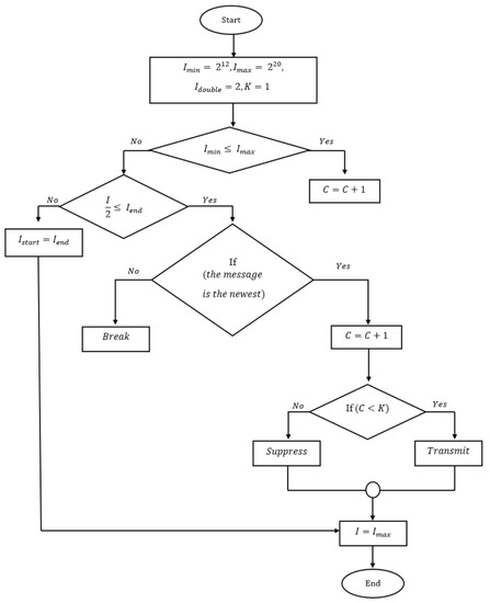
Figure 2.
Flowchart of each interval of trickle timer algorithm.
3. Related Work
A novel technique was suggested by [11], which focused on the case of inconsistency in its amendment. More precisely, the primary target was to select random time t from [0, Imin] instead of selecting it from [I/2, I]. When a consistent state is obtained at the vertex, the listening period is only canceled from the first interval, and the consistent state is then chosen from the main interval range [I/2, I]. However, the study made an unrealistic hypothesis: to have a 100% energy-consuming duty cycle. In addition, the algorithm modification did not eliminate the listening-only period. However, it is still present in the sub-periods.
A new approach was suggested by [13], which is called the “E-Trickle” algorithm. This approach established the main goals of the suppression process by eliminating the listen-only period and canceling vertices to receive the control message from the time t that is randomly picked until the termination of the time interval. The researchers proposed three adjustments to address the short-listen issue without using the listen-only phase in the trickling approach. The first modification randomly selected the random time t from the period [I/2, I], which is chosen from [0, I]. The second modification was the counter c value, which begins with zero at the start of the first period Imin rather than being set to zero at the start of each period. The final change was the redundancy factor k value, determined by the period size. Consequently, the short length of the period will have the priority to carry more than the long length of the period in case of unequal node periods. As a result of the research, the convergence time decreases for a given number of vertices, loss rate, and k value. However, considering the different number of vertices and various k and loss ratio values, no discernible differences in average energy consumption or packet delivery ratio have been observed. The IETF ROLL group [16] advised against using different values of k, which produces a developing load imbalance and consumes more energy. Nonetheless, several values of k were used in the study.
The main target of the trickle timer explained by [19] is to broadcast and update all vertices in WSN; thus, the vertex dominates the propagation by recording the number of packets rather than flooding. The vertex should halt propagation if it loads the same updated code. As a result, the trickle became a contemporary information dissemination method used in various applications.
One of the critical goals of the trickle algorithm is to maintain short convergence times, which is accomplished by reducing the quantity of routing updates that need to be propagated. [20]. The “Trickle-F” algorithm was proposed by [20] based on the trickle algorithm. The primary objective of this technique is to completely stop the broadcast to find every possible routing path. An idea appears from the notion that the trickle is insufficient for routing. While flow of the trickling strategy employed a non-deterministic suppression message; that required some vertices to remain inactive for an extended duration of time, it keeps the vertex unidentified. When priority factors were introduced to the traditional algorithm, they enhanced the transmission priority for vertices that had waited for transference for a longer time in the preceding interval. More precisely, a vertex with a higher s-value will send more because the s-value is the divisor in the dispatch time relation. The results of this experiment demonstrated that improved routes are discovered with fewer vertices and the same average amount of power utilized. In other words, a lower power consumption might be used to provide paths of the same quality. A modification that solves the load balancing issue. However, it is still caught in the drawn-out listening-only period’s extended convergence time.
Lin et al. [21] proposed an adaptive trickle technique. This study investigated routing performance in the case where residual power was minimal and became less than the energy threshold realized in WSN. The primary goal of this study was to create a parameter for a dynamic trickle timer that operates in safe mode and with highly minimal energy. The study initially tested various values of Imin, starting with small ones. The study then analyzed and evaluated the convergence time and found that a small value of Imin would result in high energy consumption and a high transmission rate with a low convergence time. After that, it was tested with greater values of Imin and found that they performed better at convergence time, especially for networks with low energy and low power consumption.
Moreover, the study evaluated several values for k and discovered that as k grew, the convergence time decreased and the average consumed energy increased. The findings of the study were promising. However, using the same techniques in the future will be difficult because the researchers employed the test bed method for experimentation, which is costly.
The trickle technique has two significant drawbacks: expanding high energy to configure a network or having a long convergence time with low energy. Ghaleb et al. [22] introduced a novel solution to solve these problems and created a new technique, which is called trickle plus. The main objective of this study [22] was to have low energy consumption when composing a network regarding the short convergence time by inserting three configuration parameters. The first parameter is a Shift Factor (SF), which specifies how many doubling periods must be surpassed; the second parameter is an IShift Start (ISS), which indicates when shifting will begin; and finally, the shift End (ISE) indicates when shifting will cease. These factors influence the trickle method’s doubling step. Consequently, the parameters in the suggested approach allow the procedure to begin with a little time shift forward to a specified period required to link without motion throughout unnecessary intervals. By using this technique, the network may be set up quickly and with minimal energy consumption.
A new solution was introduced by [23] to solve problems related to the listen-only period, which is called the Elastic Trickle Timer Algorithm. The presented algorithm was put out for the appropriate allocation of the listen-only period, which is dependent on network density, thus reducing power consumption and enhancing convergence time.
Reference [24] introduced a novel solution to the restrictions created by RPL’s short listening duration, which causes network inconsistency. Frequent inconsistencies caused a high rate of dropped packets and a rise delay in the network. Reference [24] proposed a new modification of the dynamic trickle algorithm to determine the listening period of the trickle timer depending on a new factor called dropping rate. The study concluded that if the dropping rate is high in a dense network, then more listening periods and less time should be used, and vice versa.
Table 1 illustrates the comparison between selected previous studies in terms of their advantages and disadvantages.

Table 1.
Related studies comparison.
4. Proposed Algorithm (Elastic Hop Count Trickle Timer Algorithm)
According to the prior section, the primary drawback of the original trickle algorithm is the listen-only period. We are curious if there is a link between the number of hops (rank) and the length of the listen-only period. The central concept was investigated to see if the number of hops has an impact on the listening period.
A novel trickle algorithm was introduced in this study called the “Elastic Hop Count Trickle Timer Algorithm.” It was carried out to let the original trickle algorithm work in a dynamic manner.
The primary contribution is the ability to dynamically choose the listen-only duration based on the number of hops needed to reach a node. Every time a node starts running, the number of hops is calculated. Every main interval starts with an Imin value, which is also the beginning of the first sub-interval. The node transmits a message within a short time of listening; the idea was implemented to make it easier for a node to join the DODAG quickly. This is the first step in making the algorithm behave in an elastic and flexible manner.
The listen-only period of the sub-interval is determined based on the node’s rank. The listen-only period will be short when the rank value is low, and vice versa. For example, suppose nodes are called n1, n2, and n3. If the rank (r1) of n1 is less than the rank (r2) of n2 then the algorithm will dynamically make the listen-only period (lp1) of n1 shorter than the listen-only period (lp2). As a relation, if r1 < r2 < r3, then this leads to the formation of lp1 < lp2 < lp3. By allowing sufficient time for the nodes to be heard, this concept helps prevent collisions.
The node utilizes the listening time to determine if its state is consistent or inconsistent based on the listen-only period that is dynamically selected. In case a node receives a new message with an unknown ID, and other nodes exchange the same message, it is considered to be in a consistent state. However, the node is regarded as inconsistent if the unknown ID of the received message is lower than the ones being exchanged by neighboring nodes.
In addition, the node tests the counter value and compares it to the k value; if the counter value is smaller than k, the node sends the message. Otherwise, the node will remain muted until the new sub-interval has been doubled and the current sub-interval has ended, as shown in Figure 3.
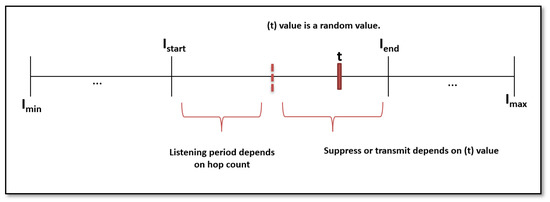
Figure 3.
Elastic Hop Count Trickle Timer Algorithm of a node.
The flowchart of the Elastic Hop Count Trickle Timer Algorithm is illustrated in Figure 4a,b.
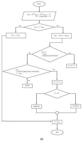
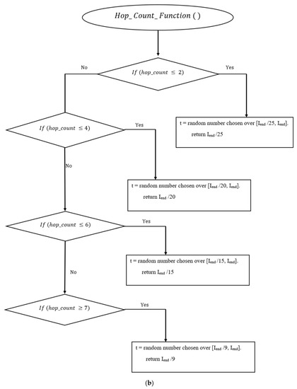
Figure 4.
(a). Flowchart of the proposed algorithm. (b). Flowchart of the proposed algorithm (Hop count function call).
5. Simulation Results and Discussion
Cooja Simulator version 3.0 was used to evaluate the performance of the routing protocol for low power and lossy networks (RPL) under the standard trickle timer algorithm, the enhanced trickle (E-trickle) algorithm, the dynamic algorithm, and the new proposed algorithm that is called the elastic hop count trickle timer algorithm.
The experiments consist of 20 and 40 nodes that are categorized as light network density. All nodes are set in both random and grid topologies under (100 m × 100 m) dimensions. If nodes are set randomly, it means that they are set in a random location with a diverse distance between the neighbors’ nodes. However, in the case of nodes, they are set in a grid topology, which means they are set with equal distance. Each experiment is run five times to get an accurate outcome.
This research assumed that the transmission range of each node was 30 m. The transmission success ratio (TX) employed is 100%, with distinct values of reception success ratio (RX) of 20%, 40%, 60%, 80%, and 100%. Table 2 shows the employed parameters in this research. The values were selected as in previous studies.
Table 2.
Simulation parameters.
The main measurement factors used to measure the algorithm’s performance are convergence time, packet delivery ratio, and power consumption.
- Convergence time
The first factor in measuring an algorithm is the convergence time, which means the time spent to build up the DODAG in the algorithm.
- b.
- Packet Delivery Ratio (PDR)
The second factor in measuring the behavior of an algorithm is the Packet Delivery Ratio (PDR), which is the ratio of the number of messages received divided by the number of messages sent. When the ratio is one, it means it is the best value.
- c.
- Power Consumption
Power consumption represents the consumed energy of nodes while moving and communicating in a specific low power and lossy network.
6. Results of Random Topology
In a random topology, the nodes were placed randomly in 1000 m2 of area. Figure 5 displayed the scenarios of light network density, where all nodes are spread randomly. There are only two kinds of nodes that are employed in this research. One sink node is set in the middle, and the other nodes are sender nodes.
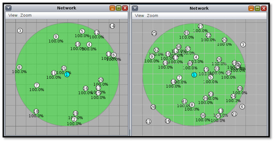
Figure 5.
Scenarios of randomly placed nodes (20 and 40).
6.1. Convergence Time
6.1.1. Convergence Time of 20 Nodes
As shown in Figure 6, it is obvious that the original algorithm is the slowest in building up the DODAG because the listen-only period of the original algorithm is too long; after the listening period, the communication between nodes starts. Moreover, as displayed in Figure 5, the best convergence time is reached by the elastic hop count algorithm rather than by the dynamic algorithm, and after that by the e-trickle algorithm. Focusing on the elastic hop count algorithm, the convergence time takes almost 80% less time than the original algorithm in building DODAG because the listen-only period was divided into intervals depending on the hop count. On the other hand, we note that when RX values decrease, the convergence time increases because external influences may play a larger role in transmission success, which makes the convergence time in building a DODAG longer.
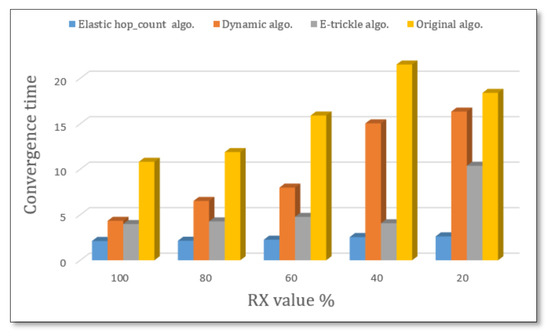
Figure 6.
Convergence time for 20 nodes with various RX values.
6.1.2. Convergence Time of 40 Nodes
After studying the convergence time behavior of the four algorithms, we found that the original algorithm also took the longest time to build up the DODAG. However, it took less time than the 20 nodes did. This leads us to conclude that when nodes become more numerous, the convergence time decreases because more surrounded nodes mean more neighbors to get the messages from; thus, it is faster to build the relations or communications between nodes.
Although, as illustrated in Figure 7, we noticed that the elastic hop count algorithm reached the best convergence time since it depends on the hop count. When hop increases, the listen-only period also increases to control the DIO messages between nodes and to build up the DODAG. Then, the dynamic algorithm takes the best convergence time after the elastic hop count; then, the e-trickle algorithm took almost half the time that the original algorithm did.
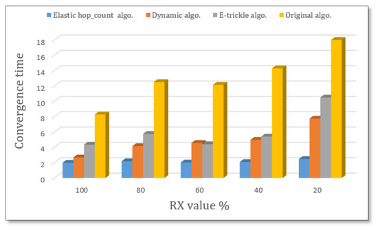
Figure 7.
Convergence time for 40 nodes with various RX values.
In conclusion, the best time is reached by the algorithm that can control the listen-only period in a good manner.
6.2. PDR
6.2.1. PDR of 20 Nodes
Comparing the behavior of the elastic hop count algorithm PDR of 20 nodes with the original algorithm, the e-trickle algorithm, and the dynamic algorithm in Figure 8, we find that the elastic hop count algorithm has the best PDR among the four algorithms in receiving the messages, even if the value of RX decreases. The elastic hop count algorithm behaves the best. At the same time, the original algorithm gives the worst PDR behavior. This is a good indication that using the elastic hop count algorithm in a turbulent environment guarantees good message reception.
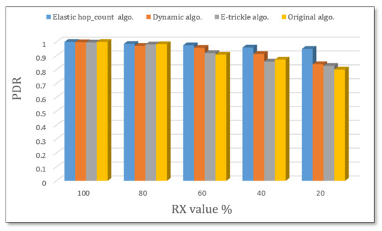
Figure 8.
PDR for 20 nodes with various RX ratios.
6.2.2. PDR of 40 Nodes
Figure 9 illustrates the PDR of 40 nodes with various RX values; it is clear that the PDR of the elastic hop count algorithm has the best values compared with the original algorithm, the dynamic algorithm, and the e-trickle algorithm. The stability of the elastic hop count algorithm is evident even if the RX values decrease.
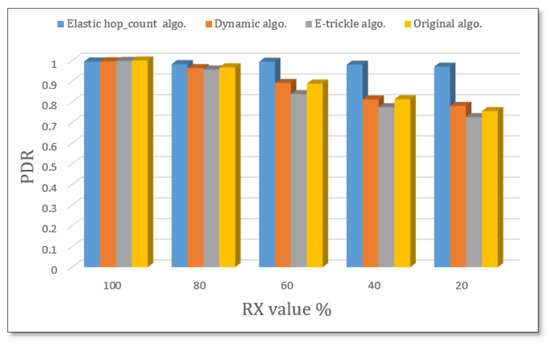
Figure 9.
PDR for 40 nodes with various RX ratios.
We conclude that the elastic hop count algorithm is stable in different reception environments.
6.3. Power Consumption
6.3.1. Power Consumption of 20 Nodes
As illustrated in Figure 10, the proposed algorithm has the lowest consumed power compared with the original, e-trickle, and dynamic algorithms. More precisely, because controlling the listen-only period in the suggested algorithm depends on the number of hop counts, the elastic hop count algorithm consumes less power, about 5% less compared with the original algorithm.
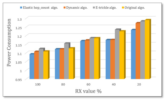
Figure 10.
Power consumption for 20 nodes with different RX ratios.
6.3.2. Power Consumption of 40 Nodes
As shown in Figure 11, when RX values decrease, the power consumption increases. The best power consumption was gained at RX equal to 100, then the power consumption increases regularly, which leads us to conclude that if external influences on the nodes increase, more power will be consumed because more nodes are communicating with each other in a short amount of time.
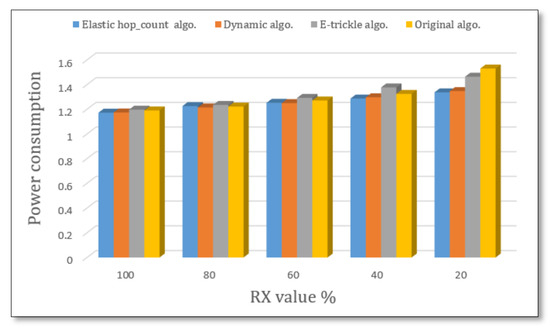
Figure 11.
Power consumption for 40 nodes with different RX ratios.
7. Results of Grid Topology
7.1. Convergence Time
7.1.1. Convergence Time of 20 Nodes
The elastic method performs better than the original in terms of convergence time, and it can construct the DODAG in roughly one-fifth of the time required by the traditional. Comparing Figure 12 with Figure 7, it is obvious that the convergence time for 20 nodes in a random topology takes, on average, less time than the convergence time spent in a grid topology since the distance between nodes is constant in the grid topology.
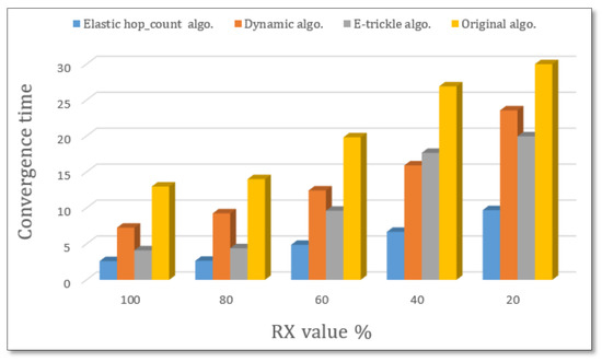
Figure 12.
Convergence time for 20 nodes with various RX values.
7.1.2. Convergence Time of 40 Nodes
As shown in Figure 13, the time needed to build the DODAG for 40 nodes is less time spent compared with 20 nodes. The main reason is that less distance between the 40 nodes in the same area leads to faster communication between nodes. However, the convergence time for 40 nodes in a random topology is less than the time in a grid topology. In conclusion, using the elastic algorithm, a grid topology on a network spent more convergence time than in random topology using the same scenario.
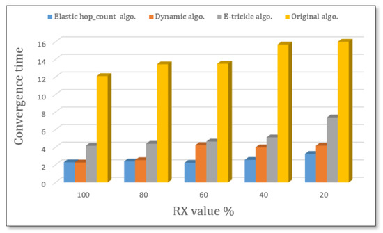
Figure 13.
Convergence time for 40 nodes with different RX values.
7.1.3. PDR of 20 Nodes
The elastic algorithm helps deliver the packets at a very high ratio. As shown in Figure 14, when the RX value is 100, the PDR is 100%. However, when the RX value is 80, the elastic algorithm’s PDR is 100%, while it is about 95% using original, dynamic, and e-trickle. Even if the RX values are low, the PDR values are high, which is a good indication that the packet loss is low even if the external influences are high under grid topology.
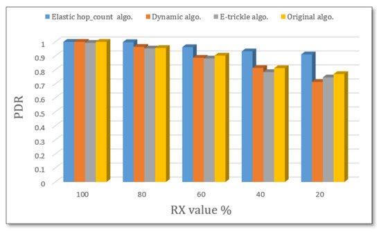
Figure 14.
PDR for 20 nodes with different RX ratios.
7.1.4. PDR of 40 Nodes
The PDR outcomes for the 40 nodes scenario, as described in Figure 15, are much closer to the 20 nodes scenario, even though it is better. When comparing between 20 and 40 nodes in terms of PDR, we notice that more nodes lead to higher PDR because more nodes mean more places to get the packets from. However, the PDR in random topology delivered better than in grid topology.
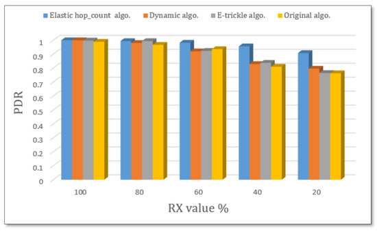
Figure 15.
PDR for 40 nodes with different RX ratios.
7.1.5. Power Consumption of 20 Nodes
The power consumption in Figure 16 is almost the same for original, e-trickle, and dynamic algorithms under 100, 80, and 60 RX values. However, the elastic algorithm consumed less power. Moreover, when RX values are 40 and 20, the elastic algorithm consumes less power than the other algorithms. The energy consumed using random topology under 100 and 80 RX values is almost the same as grid topology. However, under 60, 40, and 20 RX values, using grid topology consumed less power than random topology in a 20 node scenario.
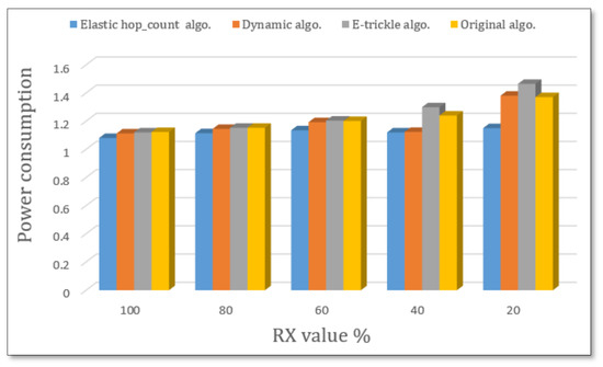
Figure 16.
Power consumption for 20 nodes with different RX ratios.
7.1.6. Power Consumption of 40 Nodes
As illustrated in Figure 17, the elastic algorithm consumed less power than dynamic, e-trickle, and original algorithms. The power consumed in a scenario of 40 nodes is greater than the power consumed in a scenario of 20 nodes because more nodes mean more communication that consumes power. In addition, the energy consumed using grid topology is almost the same as the power consumed using random topology on 40 nodes.
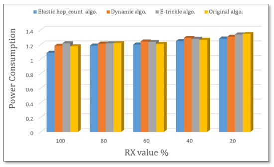
Figure 17.
Power consumption for 40 nodes with different RX ratios.
8. Conclusions
One of the core elements of the routing protocol for low power and lossy networks (RPL) is the trickle timer method. The trickle algorithm directly controls and affects the time a message takes to arrive from one node to another. It has a listen-only period, which causes load imbalance, node inconsistencies, and node slowness in the trickling algorithm. Previous studies provided positive outcomes, but there are several restrictions on trickle timer performance. The fundamental limitation of a trickle timer is a long listen-only period, leaving the node listening for an extended amount of time without the opportunity to send before the period ends, causing a high delay in the network.
This study introduced the “Dynamic Hop Count,” which is a novel Trickle Timer Algorithm. It took care of the listen-only period limitations by controlling the trickle time using the number of hops between nodes (hop counter factor), then calculating the listen period according to it.
The method was evaluated using a variety of measurement parameters, including the packet delivery ratio (PDR), power consumption, and convergence time under random and grid topologies.
The proposed algorithm significantly improved convergence time by joining DODAGs and conserving power with a high PDR compared with the previously available trickle timer algorithms and according to the outcomes.
In future work, we are looking to make the algorithm more secure by applying the algorithm on real testbeds and studying the performance using parallel servers.
Author Contributions
Data curation, M.R.A.-H.; Formal analysis, R.M., E.M. and O.A.; Investigation, M.R.A.-H.; Methodology, R.M. and E.M.; Project administration, R.M.; Resources, R.M. and E.M.; Software, B.A.; Validation, B.A.; Visualization, O.A.; Writing—original draft, R.M. and E.M.; Writing—review & editing, B.A., M.R.A.-H. and O.A. All authors have read and agreed to the published version of the manuscript.
Funding
This research received no external funding.
Institutional Review Board Statement
Not applicable.
Informed Consent Statement
Not applicable.
Data Availability Statement
Not applicable.
Conflicts of Interest
The authors declare no conflict of interest.
References
- Madakam, S. Internet of Things: Smart Things. Int. J. Future Comput. Commun. 2015, 4, 250–253. [Google Scholar] [CrossRef]
- Li, S.; Xu, L.D.; Zhao, S. The Internet of Things: A Survey; Springer: Berlin/Heidelberg, Germany, 2015; Volume 17, pp. 243–259. [Google Scholar]
- Atzori, L.; Iera, A.; Morabito, G. The Internet of Things: A Survey. Comput. Netw. 2010, 54, 2787–2805. [Google Scholar] [CrossRef]
- Alzaqebah, A.; Al-Sayyed, R.; Masadeh, R. Task scheduling based on modified grey wolf optimizer in cloud computing environment. In Proceedings of the 2019 2nd International Conference on New Trends in Computing Sciences (ICTCS), Amman, Jordan, 9–11 October 2019; IEEE: Piscataway, NJ, USA, 2019; pp. 1–6. [Google Scholar]
- Albalas, F.; Al-Soud, M.; Almomani, O.; Almomani, A. Security-aware CoAP application layer protocol for the internet of things using elliptic-curve cryptography. Power (Mw) 2018, 1333, 151. [Google Scholar]
- Almomani, O.; Al-Soud, M.; Almomani, A. Secure and Energy-effictive CoAP Application Layer Protocol for the Internet of Things. Power (Mw) 2017, 1333, 151. [Google Scholar]
- Winter, T.; Thubert, P.; Brandt, A.; Clausen, T.; Hui, J.; Kelsey, R.; Levis, P.; Pister, K.; Struik, R.; Vasseur, J. RPL: IPv6 Routing Protocol for Low power and Lossy Networks. RFC 6550, IETF ROLL WG. 2012. Available online: https://www.rfc-editor.org/rfc/rfc6550.html (accessed on 20 July 2022).
- Saaidah, A.; Almomani, O.; Al-Qaisi, L.; Alsharman, N.; Alzyoud, F. A comprehensive survey on node metrics of RPL protocol for IoT. Mod. Appl. Sci. 2019, 13, 1. [Google Scholar] [CrossRef][Green Version]
- Saaidah, A.; Almomani, O.; Al-Qaisi, L.; Madi, M.K. An efficient design of RPL objective function for routing in internet of things using fuzzy logic. Int. J. Adv. Comput. Sci. Appl. 2019, 10, 184–190. [Google Scholar] [CrossRef]
- Ayed, R.B.; Gara, F.; Hamida, E.B.; Saad, L.B.; Tourancheau, B. An adaptive timer for RPL to handle mobility in wireless sensor networks. In Proceedings of the 2016 International Wireless Communications and Mobile Computing Conference (IWCMC), Paphos, Cyprus, 5–9 September 2016; IEEE: Piscataway, NJ, USA, 2016. [Google Scholar]
- Djamaa, B.; Richardson, M. Optimizing the Trickle Algorithm. IEEE Commun. Lett. 2015, 19, 819–822. [Google Scholar] [CrossRef]
- Yassein, M.O.B.; Hmeidi, I.; Shehadeh, H.; Yaseen, W.B.; Esra’a Masa’deh Mardini, W.; Baker, Q.B. Performance Evaluation of “Dynamic Double Trickle Timer Algorithm” in RPL for Internet of Things (IoT). In Proceedings of the IoTBDS 2019, Crete, Greece, 2–4 May 2019; pp. 430–437. [Google Scholar]
- Ghaleb, B.; Al-Dubai, A.; Ekonomou, E. E-Trickle: Enhanced Trickle Algorithm for Low- Power and Lossy Networks. In Proceedings of the 14th IEEE International Conference on Ubiquitous Computing and Communications, (IUCC-2015), Liverpool, UK, 26–28 October 2015; pp. 1123–1129. [Google Scholar]
- Masadeh, R.; Alsharman, N.; Sharieh, A.; Mahafzah, B.A.; Abdulrahman, A. Task scheduling on cloud computing based on sea lion optimization algorithm. Int. J. Web Inf. Syst. 2015, 17, 99–116. [Google Scholar] [CrossRef]
- Abu Khurma, R.; Almomani, I.; Aljarah, I. IoT Botnet Detection Using Salp Swarm and Ant Lion Hybrid Optimization Model. Symmetry 2021, 13, 1377. [Google Scholar] [CrossRef]
- Levis, P.; Clausen, T.; Hui, J.; Gnawali, O.; Ko, J. The Trickle Algorithm. RFC 6206, Internet Engineering Task Force (IETF). 2011. Available online: https://citeseerx.ist.psu.edu/viewdoc/download?doi=10.1.1.478.977&rep=rep1&type=pdf (accessed on 1 August 2022).
- Kumar, J.S.; Suresh, D. Design and implementation of a mobility support adaptive trickle algorithm for RPL in vehicular IoT networks. Int. J. Ad. Hoc. Ubiquitous Comput. 2022, 40, 38–49. [Google Scholar] [CrossRef]
- Bani Yassein, M.; Aljawarneh, S.; Ghaleb, B.; Masadeh, E.; Masadeh, R. A new dynamic trickle algorithm for low power and lossy networks. In Proceedings of the 2016 International Conference on Engineering & MIS (ICEMIS), Agadir, Morocco, 22–24 September 2016; IEEE: Piscataway, NJ, USA, 2016; pp. 1–6. [Google Scholar]
- Levis, P.; Patel, N.; Culler, D.; Shenker, S. Trickle: A Self-Regulating Algorithm for Code Propagation and Maintenance in Wireless Sensor Networks; Computer Science Division; University of California: Berkeley, CA, USA, 2003. [Google Scholar]
- Vallati, C.; Mingozzi, E. Trickle-F: Fair broadcast suppression to improve energyefficient route formation with the RPL routing protocol. In Proceedings of the Sustainable Internet and ICT for Sustainability (SustainIT), Palermo, Italy, 30–31 October 2013; pp. 1–9. [Google Scholar]
- Lin, Y.; Wang, P. Ubiquitous Computing Application and Wireless Sensor; Springer: Amsterdam, The Netherlands, 2015; Chapter 16; Volume 331, pp. 163–173. ISBN 978-94-017-9618-7. [Google Scholar]
- Ghaleb, B.; Al-Dubai, A.; Ekonomou, E.; Paechter, B.; Qasem, M. Trickle-Plus: Elastic Trickle Algorithm for Low-Power Networks and Internet of Things. In Proceedings of the 2016 IEEE Wireless Communications and Networking Conference Workshops (WCNCW), Doha, Qatar, 3–6 April 2016; pp. 1–7. [Google Scholar]
- Yassein, M.B.; Aljawarneh, S. A new elastic trickle timer algorithm for Internet of Things. J. Netw. Comput. Appl. 2017, 89, 38–47. [Google Scholar] [CrossRef]
- Yassein, M.B.; Krstic, D. Optimized Dynamic Trickle Algorithm for Low Power and Lossy Networks. IEICE Proceedings Series; 64(ICTF2020_paper_11). 2021. ISSN 2188-5079. Available online: https://www.ieice.org/publications/proceedings/summary.php?iconf=ICTF&session_num=ICTF_2&number=ICTF2020_paper_11&year=2020 (accessed on 1 August 2022).


Publisher’s Note: MDPI stays neutral with regard to jurisdictional claims in published maps and institutional affiliations. |
© 2022 by the authors. Licensee MDPI, Basel, Switzerland. This article is an open access article distributed under the terms and conditions of the Creative Commons Attribution (CC BY) license (https://creativecommons.org/licenses/by/4.0/).