Model for Determining Noise Level Depending on Traffic Volume at Intersections

Abstract

The negative external effects caused by traffic growth have been recognized as the main factors that degrade city quality of life. Therefore, research around the world is being conducted to understand the impact of traffic better and find adequate measures to reduce the negative impact of traffic growth. The central part of this research consists of mathematical models for simulating the negative consequences of congestion and noise pollution. Four non-linear models for determining noise levels as a function of traffic flow parameters (intensity and structure) in the urban environment were developed. The non-linear models, including two artificial neural networks and two random forest models, were developed according to the experimental measurements in Novi Sad, Serbia, in 2019. These non-linear models showed high anticipation accuracy of the equivalent continuous sound level (Laeq), with R² values of 0.697, 0.703, 0.959 and 0.882, respectively. According to the developed ANN models, global sensitivity analysis was performed, according to which the number of buses at crossings was the most positively signed influential parameter in Laeq evaluation, while the lowest Laeq value was reached during nighttime. The locations occupied by frequent traffic such as Futoska and Temerinska positively influenced the Laeq value.

1. Introduction

According to the World Health Organization, noise significantly affects the psychophysical health of the urban population [1]. On average, more than 50% of the population in urban areas is exposed to non-stop levels of noise that exceed 55 dBA, whereas >15% of the population is exposed to levels that exceed 65 dBA. In the European Union, around 94 million people in urban environments and around 31 million people outside urban environments are endangered by traffic noise, of which approximately 112 million people are exposed to elevated noise levels caused by road traffic [2,3]. Research indicates that unwanted sound seriously affects cardiovascular, immunological, central, and vegetative nervous and digestive systems [4,5,6,7]. The most severe health impacts from noise exposure (morality, insomnia, cardiovascular) are experienced by a relatively small proportion of the population, but a larger number of people experiences feelings of discomfort or stress. Generally, noise effects can be direct, such as hearing loss, or indirect, such as disturbance of activities, sleep and communication. Physiological stress reactions are mainly manifested through the autonomic nervous system (sympathetic nerve) and endocrine system (pituitary gland, adrenal gland). Risk factors such as blood pressure, hypertension, arteriosclerosis and ischemic heart diseases, etc., are mainly related to negative noise environments [8]. Many risk factors related to noise exposure are still to be discovered but the main health concern related to noise was, for a long time, occupational exposure and hearing loss. The World Health Organization (World Health Organization, 1999, 2009, 2011) determined that the equivalent 8-h exposure threshold for hearing loss includes impulse sounds of 75 dBA. It is important to state that noise has a cumulative impact on many health issues, including hearing lose, as people are exposed to noise throughout their lifetime and hearing damage can build over time. Due to this cumulative impact over time, in many cases, noise is not directly related with health issues and goes unnoticed. Negative effects can also be found in the economic sphere through the negative impact on the real estate market, which experiences a significant drop in given zones [9,10,11]. Based on the stated facts, it can be concluded that road traffic is the dominant source of noise pollution [12,13].

Through this paper, we have defined a model which correlates traffic intensity and structure with the intensity of noise caused by traffic at urban intersections.

The existing global practice uses different models for predicting road traffic noise, such as empirical models [14], comparison of road traffic noise prediction models (CoRTN) [15], German standard (Richtlinien für den Lärmschutz an Straben), RLS-90 [16] and NMR-96 [17], etc. They are adapted to the characteristics of the vehicle fleet of the urban environment for which they were developed. In addition, almost all models and research are focused on traffic sections far from traffic lights, intersections, and pedestrian crossings, where it can be assumed that motor vehicles move at a constant speed in accordance with the general limit vehicle speed of 50 km/h. Urban politics in Serbia is increasingly focused on pedestrian safety, so the number of sections with traffic lights and pedestrian crossings is highly increasing. For example, in the city of Novi Sad (urban population of 277.522), there are more than 100 locations with traffic lights and pedestrian crossings, and that number is increasing every year. Experimental results of measuring noise levels in the Republic of Serbia [18] significantly deviate from the values which the given models can obtain. This indicates a need to develop a new model more suitable for local traffic conditions (vehicle fleet is far older than in the EU, etc.).

Considering that intersections are critical elements of road networks in terms of air quality impact [19], we have focused our research on these traffic sections, intersections with traffic lights, and pedestrian crossings. Since vehicle movement and speed are highly limited at these sections (less than 20 km/h), the surface texture is not the most influential factor in tire/road noise generation [20,21]. Furthermore, a noise level model was generated using all vehicles at the intersection (from all four approaches). This fact led us to the need for a new model focusing on engine noise and vehicle sirens, etc.

Noise levels were analyzed in a scenario that included drive-through (green traffic light and 50 km/h vehicle speed without stopping) and stop-and-go (red-to-green traffic light and vehicles that stop and start driving again). As a result, a more detailed categorization of motor vehicles is introduced, while the correction factor is determined for more accurate predictions and efficient traffic flow management. In addition, territorial and social traffic parameters (age of the vehicle fleet, road type, quality and “traffic etiquette” of participants) were also analyzed according to possibilities.

Based on the experimental results’ measurements of equivalent noise levels and publicly accessible data in the city of Novi Sad, a functional connection was established between the selected traffic flow and equivalent noise level at a reference distance from the crossroad axes. The ability to use publicly accessible data (annual measurements of noise levels [22], annual studies of traffic counting at intersections [23], etc.) and vehicle counting system data, etc., to generate a useable prediction of traffic conditions [24] and noise levels in the observed environment is one of the basic characteristics of the enclosed model. The model can be used quite efficiently by various parties, such as designers, architects, and even real-estate agents/buyers.

The methodology used in the realization of the study is in complete accordance with the EU Commission’s policies for estimating noise exposure, mapping and analyzing the related data on noise exposure [25,26,27]. Furthermore, all of the existing studies and research conducted in Novi Sad concerning noise analysis and traffic counting, as well as other analyses (counting public transport passengers, analysis of vehicle speed on the street network, city parking analysis, household surveys, etc.) were analyzed.

Recently, artificial neural network (ANN) models were applied to estimate urban noise prediction [28,29].

The ANN models were capable of predicting urban noise with increased precision. Despite a slight reduction in the exactness of the acquired results, the values received by the ANN models were also quite acceptable. The developed models employed activation functions to estimate the noise level according to the set of input variables and are adjusted to the environment in which the models were constructed to evaluate the traffic noise [28].

Several studies have demonstrated this technique’s suitability in reliable traffic noise predictions [28,30,31,32,33].

The number of hidden nodes influences the precision of the equivalent continuous sound level prediction, with models with fewer nodes than the starting number of nodes being better [34].

Non-linear models, including random forest regression (RFR) and ANN models, performed better than linear models, mostly because relations among examined variables were inherently non-linear. In the works by Liu et al., [35] and Staab et al., [36], the accuracy of the RFR was emphasized in predicting noise level based on the traffic volume.

In the study by Liu et al. [35], a hybrid approach was applied, combining a traffic propagation and RFR model to map the average daily total environment noise levels, with a resolution of 30 m × 30 m. Integrating deterministic and stochastic approaches could furnish precise total environmental noise assessments for extensive geographic areas where sound level measurements are obtainable.

In the study by Adulaimi et al. [37], an accurate overview of the crucial variables which exert a significant impact on traffic noise are described using computing techniques, including decision trees, random forests, linear regression and support vector regression. The results indicate that the RF model was the most efficacious and reliable at anticipating traffic noise values based on the performance analysis of the developed models and the performance criteria of R² and RMSE.

The objective of this study was to investigate the possibility of predicting noise level based on the traffic volume at intersections, using two non-linear empirical models, an artificial neural network and random forest models.

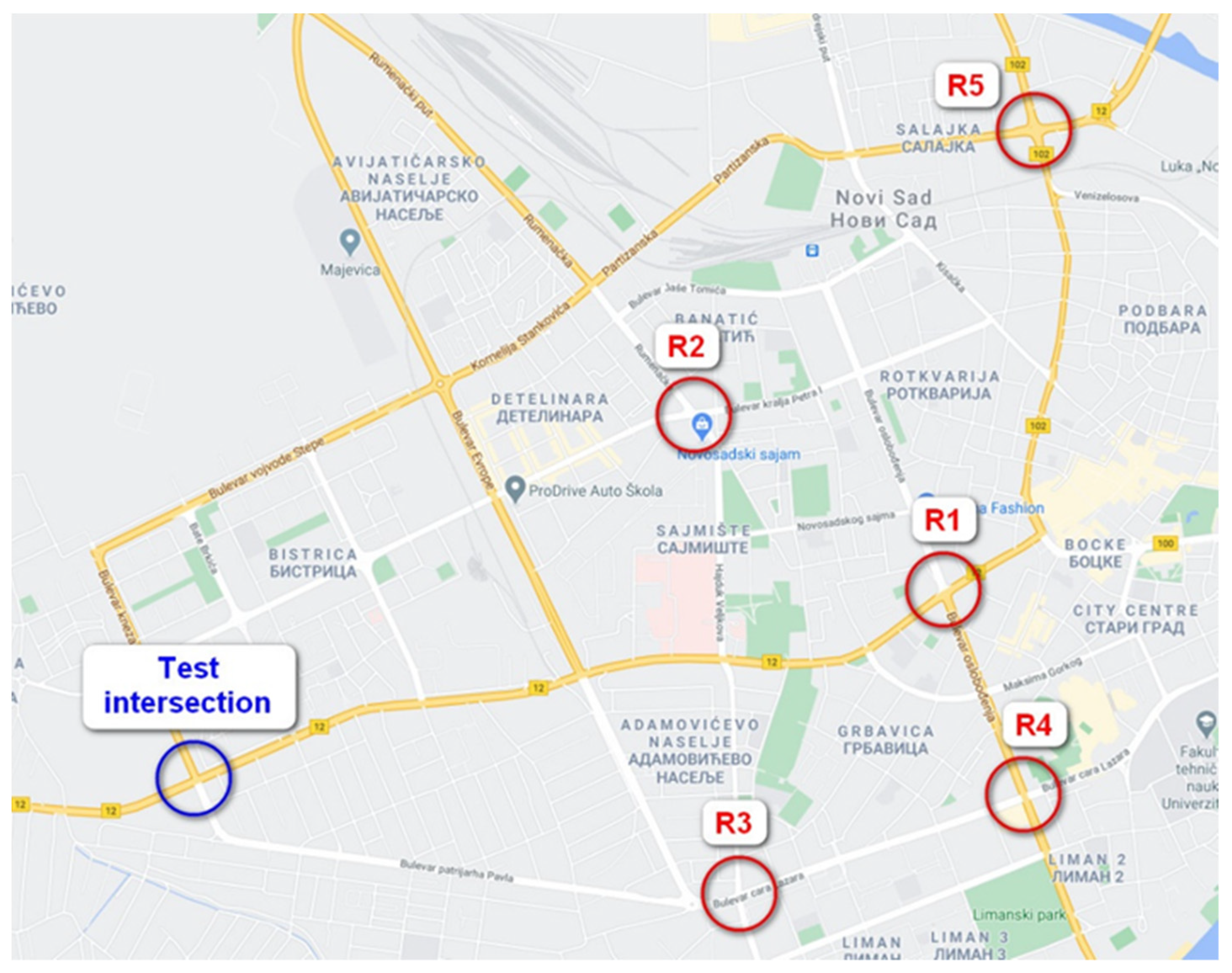
2. Materials and Methods

For this research, a total of six locations (intersections) were selected in Novi Sad, Serbia, where noise and traffic flow intensity and structure were simultaneously measured (Figure 1). Counting and measuring were performed in 24-h intervals, where five intersections were selected for forming the model, and one for testing.

The following four criteria were adopted for selecting the locations for counting and measuring noise:

• High intensity of traffic load (more than 3000 veh/h);
• Presence of trucks and buses;
• Intersection with signalization;
• Street fronts and buildings near the intersection.

Intersection R1—High and medium-height buildings at all corners, no trees, presence of buses, but no trucks, pedestrians at all approaches, traffic signals.

Intersection R2—High buildings at two of four corners, no trees, presence of buses and trucks, pedestrians at all approaches, traffic signals.

Intersection R3—High buildings at three of four corners, trees at fourth corner, presence of buses and trucks, pedestrians at all approaches, traffic signals.

Intersection R4—No high buildings around the center of the intersection, trees at one corner, presence of buses, no trucks, pedestrians at all approaches, traffic signals.

Intersection R5—No high buildings around the center of the intersection, no trees, presence of trucks and buses, pedestrians at all approaches, traffic signals.

Intersection R6 (test intersection)—No high buildings around the center of the intersection, trees at two of four corners, presence of trucks and buses, pedestrians at all approaches, traffic signals.

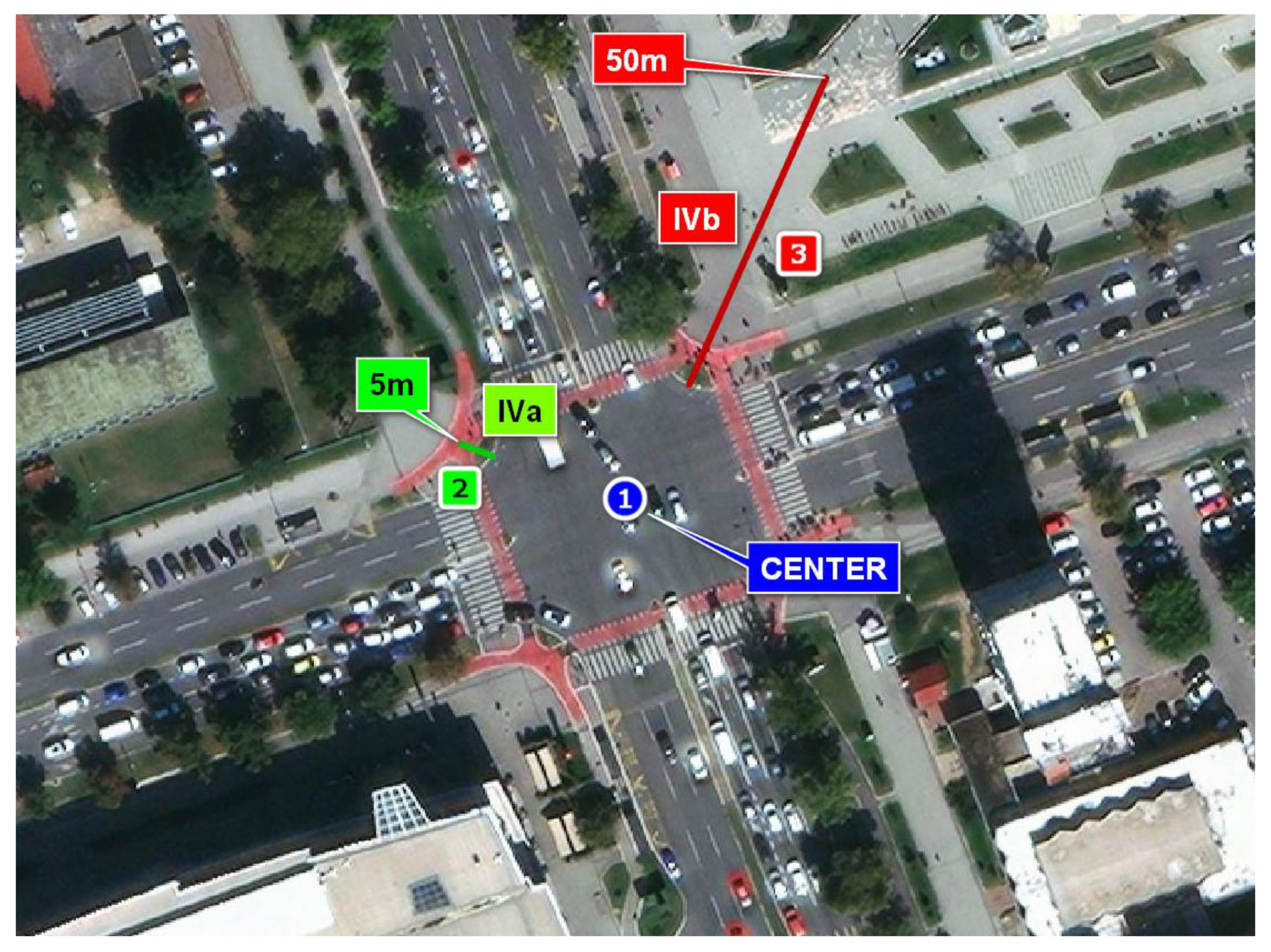
2.1. Noise Measurement Methodology

The measurement was conducted using the CESVA TA120 device (CESVA instruments S.L.U., Barcelona, Spain) during June 2019. Measurement started on 19 June 2019, and concluded on 25 June 2019. A 24-h session of noise level measurement was conducted at each location. The measurement was conducted according to the recommendations of the following regulations:

• Rulebook on the methods of noise measurement, contents and scope of the noise measurement reports, [38],
• Rulebook on the content and methods of development of strategic noise maps and the manner of their presentation to the public, [38],
• ISO Standard 1996-1:2016 [27].

Serbian regulations are in line with EU Directives 2002/49/EC and 2003/613/EC and ISO standards [27]. Therefore, noise level analysis was conducted for sequential 15-min intervals. Following the rules of The Ministry of Environmental Protection, Government of Serbia, A-weighted levels for daytime L_day, evening L_evening and nighttime L_night during a 24-h measurement period were calculated [39]. The daytime measurement interval was from 6 a.m. to 6 p.m., the evening interval from 6 p.m. to 10 p.m. and the nighttime interval from 10 p.m. to 6 a.m.

During the measurements, meteorological parameters (air temperature, precipitation, rain, etc.) that might influence noise measurement in the conducted procedure were monitored. The measurement was only conducted during intervals of consistent meteorological conditions, so the effect of the aforementioned meteorological parameters can be regarded as negligible. The measurement periods with meteorological parameters that showed significant deviations were particularly analyzed and repeated when necessary. The influence of meteorological parameters on urban noise propagation in an observed environment is a subject for further research.

One limitation of the neural network model was its reliance on acoustic measurements. The problem was that these measurements were often flawed because the sonometers did not only measure vehicle sounds, but also other sounds, which should not have been considered.

Noise level measurement was conducted on 19 June, 21 June, 24 June and 26 June 2019, because these days are common for traffic counting. Figure 2 shows the values of meteorological parameters by day during the period of noise level measurement.

For the purposes of developing the model and determining noise level reduction, simultaneous measurements were conducted at distances of 5 m and 50 m from the road’s axis using two identical measuring devices (Figure 3). The measurements confirmed the results of previous research regarding noise propagation from the road’s axis [40].

2.2. Traffic Counting Methodology

Along with recording noise levels, traffic counting was simultaneously performed at each location.

In addition to traffic volume in 15-min time intervals, data on the structure of the traffic flow were also collected. Vehicles were placed in the following categories:

-

PA—Passenger car,

-

BUS *—Bus,

-

HV *—Heavy vehicles,

-

BUS + HV *—Bus and heavy vehicles.

For the study, the vehicle categories marked with an asterisk (*) were especially significant because these vehicles produce a higher noise intensity when passing through an intersection or waiting for the green light [41].

2.3. Non-Linear Regression Models

Non-linear regression models for noise prediction and noise map calculations are widely used to represent exposure to road traffic noise. However, frequently, their accuracy and the quality of the noise estimates are sometimes limited. In a paper by Aguilera et al. [42], the application of land use regression modelling was used to investigate the long-term spatial variability of road traffic noise in an urban area within three European cities.

In an article by Ryan and LeMasters [43], a brief summary and the application of non-linear regression models was presented outlining similarities and differences of the variables included in the model, model development and model validation. This article used non-linear regression to characterize air pollution exposure and health effects for individuals residing within urban areas.

2.3.1. ANN Modeling

A multi-layer perceptron (MLP) concept, with three layers (input, hidden and output) was applied for modelling the artificial neural network model (ANN) for the prediction of noise level based on the traffic volume at intersections. In the first ANN model (ANN1), PA and HV parameters were used for the prediction of Laeq, while within ANN2 modelling, location (R1-R5) and time period (morning, noon, afternoon and night) were used as categorical variables. Parameters such as BUS, HV and PA were used as numerical variables for the ANN2 model. According to the known references, the ANN models were proven entirely suited to estimating non-linear functions [28,29,30]. Prior to computation, the input and output database was normalized to enhance the conduct of the ANN model. During this iterative process, input data were repeatedly presented to the network [44,45]. The Broyden–Fletcher–Goldfarb–Shanno (BFGS) algorithm was used as an iterative method for solving unconstrained non-linear optimization during the ANN modelling.

The experimental database for ANN was randomly divided into training, cross-validation and testing data (with 70%, 15% and 15% of experimental data, respectively). The training dataset was used for the learning cycle of ANN and also for the evaluation of the optimal number of neurons in the hidden layer and the weight coefficient of each neuron in the network. A series of different topologies was used, in which the number of hidden neurons varied from 5 to 10, and the training process of the network was run 100,000 times with random initial values of weights and biases. The optimization process was performed based on validation error minimization. It was assumed that successful training was achieved when learning and cross-validation curves approached zero.

Coefficients associated with the hidden layer (weights and biases) were grouped in matrices W₁ and B₁. Similarly, coefficients associated with the output layer were grouped in matrices W₂ and B₂. It is possible to represent the neural network by using matrix notation (Y is the matrix of the output variables, f₁ and f₂ are transfer functions in the hidden and output layers, respectively, and X is the matrix of input variables [29,40]:

$$Y=f_1(W_2\cdot f_2(W_1\cdot X+B_1)+B_2)$$

(1)

Weight coefficients (elements of matrices W₁ and W₂ and vectors B₁ and B₂) were determined during calculation in the ANN learning cycle. The values of these coefficients were revised by applying optimization procedures to minimize the error between the network and experimental outputs [44,46,47], according to the sum of squares (SOS). The well-known BFGS algorithm was used to accelerate and consolidate the convergence in the finding the solution [48]. The coefficient of determination of the ANN model was investigated as a parameter to inspect the developed ANN model’s performance.

Global Sensitivity Analysis

Yoon’s interpretation method was used to determine the relative influence of location (R1–R5), time period (morning, noon, afternoon and night), BUS, HV and PA on noise level [49]. This method was applied on the basis of the weight coefficients of the developed ANN model.

Yoon’s method of global sensitivity was used to calculate the direct influence of the input parameters on the output variables, corresponding to the weighting coefficients within the ANN model [49]:

$$R{I}_{ij}(\%)=\frac{{\displaystyle \sum _{k=0}^n(w_{ik}\cdot w_{kj})}}{{\displaystyle \sum _{i=0}^m\left|{\displaystyle \sum _{k=0}^n(w_{ik}\cdot w_{kj})}\right|}}\cdot 100\%$$

(2)

where w—denotes the weighting factor in the ANN model, i—input variable, j—output variable, k—hidden neuron, n—number of hidden neurons and m—number of inputs.

2.3.2. RFR Modeling

The random forest model (RF) is a widely used machine learning algorithm developed upon decision trees to foresee outputs according to prediction variables [50]. The RF model can be implemented for classification or regression purposes. The random forest regression method is used for the mean prediction of individual trees, consistent with decision trees developed according to the training dataset [35]. In addition, the RF model can reveal the importance of features. The RFR models were constructed upon the data presented in

Table 1. Descriptive statistics of the experimental results.

Location	Parameter	BUS	HV	BUS + HV	PA	Laeq
R1	Mean	7.792	27.729	35.521	632.521	72.206
	St.Dev.	3.744	22.480	24.736	378.003	2.943
	Min.	0	0	0	30	64.910
	Max.	16	70	81	1100	75.790
R2	Mean	13.156	47.219	60.375	584.333	69.942
	St.Dev.	6.758	36.836	41.527	332.679	4.149
	Min.	1	3	4	78	59.130
	Max.	33	118	142	1103	73.350
R3	Mean	22.021	29.635	51.656	689.719	70.305
	St.Dev.	11.635	24.512	32.992	389.268	3.695
	Min.	0	1	1	46	61.090
	Max.	43	82	109	1131	77.210
R4	Mean	12.042	27.573	39.615	783.000	68.719
	St.Dev.	6.961	20.728	25.663	409.785	3.903
	Min.	0	1	2	109	56.970
	Max.	31	73	88	1322	72.650
R5	Mean	7.417	22.115	29.531	548.240	70.233
	St.Dev.	3.873	17.965	21.104	323.031	2.093
	Min.	0	0	0	29	64.870
	Max.	14	61	75	997	72.590
R6	Mean	8.865	29.083	37.948	551.667	68.096
	St.Dev.	4.990	24.346	26.318	319.610	3.672
	Min.	0	0	1	21	55.790
	Max.	24	80	87	1009	71.660

St.Dev.—standard deviation, Min.—minimum, Max.—maximum.

. Similarly, to the ANN model, the inputs for the RFR models were traffic volume parameters at intersections. During random forest regression model calculation for the prediction of noise level, a large set of decision trees was constructed, and each tree was built according to the specific bootstrap sample within a training dataset [51]. In this study, the bootstrap function was employed to randomly divide the dataset into coherent subsets, in the training and test subsets, which covered 50% and 40% of the entire data, respectively [52]. New sub-samples were selected from the input sample dataset and multiple trees were added to the RFR structure to fit the obtained sub-samples. Throughout the training cycle, the RFR model estimated the results of the formed trees to minimize the prediction error [50]. During RFR modelling, location (R1-R5) and time period (morning, noon, afternoon and night) were used as categorical variables, while BUS, HV and PA were used as numerical variables. Over the RFR calculation, the number of trees parameter was set to 100, 200, 300, 400, 500 and 1000, while the random test data proportion was set to 40% and the sample proportion was 50%.

The ANN and RFR models were calculated utilizing StatSoft Statistica, ver. 10.0, Palo Alto, CA, USA.

2.4. The Accuracy of the Model

The computational confirmation of the constructed non-linear models was tested using standard statistical tests, such as the coefficient of determination (R²), reduced chi-square (χ²), mean bias error (MBE), root mean square error (RMSE), mean percentage error (MPE), the sum of squared errors (SSE) and average absolute relative deviation (AARD), MBE, RMSE, MPE, SSE and AARD. These commonly used parameters can be calculated as follows [52]:

$${\chi }^2=\frac{{\displaystyle \sum _{i=1}^N{(x_{\exp ,i}-x_{pre,i})}^2}}{N-n}$$

(3)

$$RMSE={\left[\frac{1}{N}\cdot {\displaystyle \sum _{i=1}^N{(x_{pre,i}-x_{\exp ,i})}^2}\right]}^{1/2}$$

(4)

$$MBE=\frac{1}{N}\cdot {\displaystyle \sum _{i=1}^N(x_{pre,i}-x_{\exp ,i})}$$

(5)

$$MPE=\frac{100}{N}\cdot {\displaystyle \sum _{i=1}^N(\frac{\left|x_{pre,i}-x_{\exp ,i}\right|}{x_{\exp ,i}})}$$

(6)

$$SSE={\displaystyle \sum _{i=1}^N{(x_{pre,i}-x_{\exp ,i})}^2}$$

(7)

$$AARD=\frac{1}{N}\cdot {\displaystyle \sum _{i=1}^N\left|\frac{x_{\exp ,i}-x_{pre,i}}{x_{\exp ,i}}\right|}$$

(8)

where x_exp,i are experimental values, x_pre,i are the model predicted values, and N and n are the number of observations and constants, accordingly.

3. Results

Based on the data collected by traffic counting and noise measurement, a comparative analysis of traffic intensity was conducted using 15-min intervals and noise values expressed in the equivalent continuous sound level—Laeq (dBA at the same time cross-sections). Figure 4 shows comparative values at the five intersections (R1–R5) used for creating the model, while the results for the sixth intersection were applied to verify the models.

Trucks and buses were placed into the same group as they have very similar noise and emission characteristics, and the preliminary statistical processing showed no significant difference in the results whether they were analyzed as separate groups of trucks, buses, or together.

By analyzing the collected data, it was determined that, in addition to traffic, other factors might influence noise intensity. One of the factors was the noise caused by poor weather conditions that occurred during the recording (wind and thunder). This parameter was eliminated by minute reports on the noise recording, so that all the instantaneous and very high values were eliminated. Measurements with longer intervals of poor weather conditions were repeated. The influence of reflection from the facades of nearby objects was eliminated due to the positioning of the measurement device and in accordance with recommendations [27]. The second factor of influence on the noise level was introduced due to the characteristics of vertical traffic signalization and street lighting, which were used as carriers for the measurement devices. The limitation that the used poles introduced mainly relates to the distance from the axis of the observed roadway, which was sometimes less than the recommended [27] (5 m instead of 7.5 m). Furthermore, it can be concluded that vibrations and audio signalization of the used traffic signalization poles also influence the measured values. By analyzing different intersections, i.e., positions of noise measurement devices compared to the observed roadways, it was determined that the correction factor amounts to 5 dB.

3.1. Mathematical Models

3.1.1. ANN1 Model

The acquired optimal neural network models showed good generalization capabilities for the experimental data and could be used to accurately predict noise level based on the traffic volume at intersections. The number of neurons for the ANN model was five (network MLP 2-5-1) to obtain the highest R² values (the R² values for prediction of output variables were 0.681, 0.692 and 0.757, for training, testing and validation cycles, respectively), as seen in

Table 2. Artificial neural network model summary (performance and errors) for training, testing and validation cycles.

Network	Performance			Error			Train. Algorithm	Error Funct.	Hidden Activation	Output Activation
	Train.	Test.	Valid.	Train.	Test.	Valid.
MLP 2-5-1	0.681	0.692	0.757	2.238	1.852	1.728	BFGS 84	SOS	Tanh	Logistic

Performance term represents the coefficients of determination, while error terms indicate a lack of data for the ANN model.

.

A comparison between experimentally obtained and model-predicted noise level values based on the traffic volume at intersections for all developed models is shown in Figure 5. The potential of the ANN1 model to predict noise level values based on the traffic volume at intersections is presented by scatter plots (Figure 5b).

The obtained ANN1 model for predicting output variables was built upon 21 weights–bias coefficients due to the high non-linearity of the observed system [53,54].

The goodness of fit between experimental measurements and model-calculated outputs, represented as ANN performance, are shown in

Table 3. The “goodness of fit” tests for the developed models.

Model	χ2	RMSE	MBE	MPE	SSE	AARD	R2	Skew	Kurt	Mean	StDev	Var
ANN1	4.160	2.038	−0.080	2.236	2367.430	1937.642	0.697	0.070	1.303	−0.080	2.038	4.153
RFR1	4.073	2.016	0.076	2.198	2318.340	1602.760	0.703	−0.056	1.391	0.076	2.017	4.067
ANN2	0.559	0.747	−0.049	0.807	320.196	652.730	0.959	0.224	2.503	−0.049	0.746	0.557
RFR2	1.837	1.354	0.016	1.357	1056.331	895.384	0.882	−0.704	3.678	0.016	1.355	1.837

.

3.1.2. ANN2 Model

The acquired optimal neural network models showed good generalization capabilities for the experimental data and could be used to accurately predict noise level based on the traffic volume at intersections. The number of neurons for the ANN model was seven (network MLP 13-7-1) to obtain the highest R² values (the R² values for prediction of output variables were 0.962, 0.943 and 0.970, for training, testing and validation cycles, respectively), as seen in Table 2.

The obtained ANN2 model for the prediction of output variables was built upon 106 weights–bias coefficients due to the high non-linearity of the observed system. The goodness of fit between experimental measurements and model-calculated outputs, represented as ANN performance, are shown in Table 3.

The acquired optimal neural network models showed good generalization capabilities for the experimental data and could be used to accurately predict noise level based on the traffic volume at intersections. The number of neurons for the ANN model was 13 (network MLP 13-13-1) to obtain the highest R² values (the R² values for prediction of output variables were 0.962, 0.943 and 0.970 for training, testing and validation cycles, respectively), as seen in Table 2.

In the literature, several studies can be found verifying the artificial neural network’s model’s ability to predict emission of traffic noise [29,55,56,57,58]. In the research by Genaro et al. [28], Laeq was evaluated utilizing street-level data sourced from Granada, Spain. The artificial neural network model results were compared with the results from other mathematical models. It was observed that predictions using the neural network outperformed the other mathematical models. Mansourkhaki et al. [34] operated ANN-MLP and ANN-RBF to evaluate Laeq according to speed, traffic volume and percentage of heavy vehicles in Tehran, Iran. By comparing the predicted outcomes, the ANN-MLP network achieved more acceptable results compared to the ANN-RBF model. Hamoda [33] applied the neural networks analysis to predict construction noise in the city of Kuwait. The results demonstrate that the general regression network-based neural models accomplished more acceptable accuracy compared to the backpropagation-established network’s results.

3.1.3. RFR Model

The acquired optimal random forest models showed good prediction capabilities for the experimental data and could be used to adequately foresee noise level based on the traffic volume at intersections. The number of trees for the RFR models was 1000 to obtain the highest R² values (during the training cycle, the R² value for the output variables was 0.882); see Table 3. The RFR and ANN models had an insignificant lack of fit tests, which means the models satisfactorily predicted output variables.

A high R² is indicative that the variation was accounted for and that the data fitted the proposed RFR model satisfactorily [59,60]. The RMSE was 1.354, and when comparing this result with RMSE for the ANN model, it can be noticed that the ANN model offered a more acceptable RMSE of 0.747. This finding is also in favor of using ANN for noise level prediction based on the traffic volume at intersections.

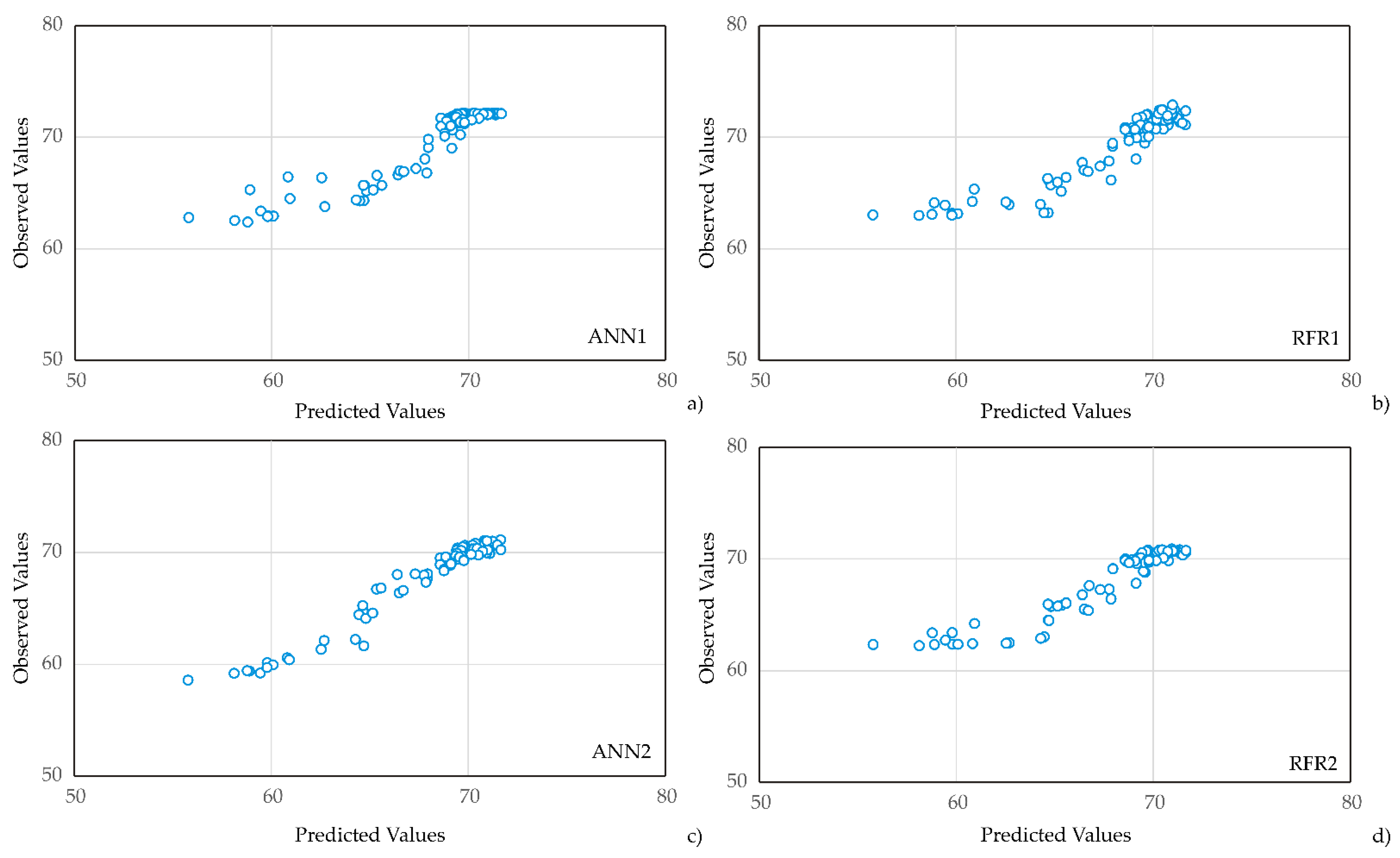
3.1.4. Model Testing

Intersection R6—Futoški put–Bulevar Kneza Miloša-Bulevar patrijarha Pavla—was selected for model testing. The presence of trucks characterizes this intersection, but for the larger part of the day, their numbers do not exceed 10% of total traffic. There are also no nearby buildings that would increase the noise level. Therefore, to compare the values acquired by the model, a control noise recording was performed at intersection R6 during a 24-h interval, on 26 June 2019. Simultaneously, traffic counting was performed in 15-min intervals, as previously shown.

Figure 6 shows that the deviations between the measured values and the values acquired with the model deviate by less than 2 dB, considering the fact that these differences are mostly less than 1 dBA. Statistically speaking, the difference of 2 dBA compared to the minimum and maximum measured noise values (min. 55.78, max. 71.66 dBA) is between:

$$\mathrm{\Delta }dBA=2.8-3.6\%$$

(9)

Every value that amounts to less than 5% of deviation can be considered a minimal deviation, that is, as a good indicator of the model’s precision.

Regardless of the model’s precision, it does have certain limitations. Namely, the model’s basic limitation is that it is bound exclusively to traffic noise, and not to noise pollution, so the occurrence of a secondary noise source may cause the data acquired by the model to significantly deviate from the actual values. During model development, a corrective value for noise caused by traffic and city infrastructure was used based on measurement; however, in situations where an intersection is surrounded by a large number of tall buildings, additional deviation from the defined value of 3–6 dBA may occur [53].

Other limitations refer to the location of noise measurement. Namely, noise that was measured and that is shown by the obtained method relates to the distance of up to 5–7.5 m from an intersection. Measurements at longer distances showed a drop in noise intensity of up to 5 dBA at 50 m from an intersection (comparative measurement). The goodness of fit between experimental measurements and model-calculated outputs for Laeq Gras location (R6), represented as ANN performance, are shown in

Table 4. The “goodness of fit” tests for the developed ANN model.

Model	χ2	RMSE	MBE	MPE	SSE	AARD	R2	Skew	Kurt	Mean	StDev	Var
ANN1	4.736	2.165	−1.729	2.668	163.033	107.967	0.877	−1.342	3.689	−1.729	1.310	1.716
RFR1	3.698	1.913	−1.346	2.273	177.343	112.211	0.872	−1.262	3.898	−1.346	1.366	1.867
ANN2	0.446	0.664	−0.038	0.762	42.234	48.705	0.968	−0.412	2.170	−0.038	0.667	0.445
RFR2	1.918	1.378	−0.426	1.377	166.464	88.218	0.898	−1.929	5.493	−0.426	1.317	1.734

.

The potential of the ANN model to predict calculated outputs for Laeq Gras location is presented by scatter plots (Figure 6). The goodness of fit between experimental measurements and model-calculated outputs for Laeq Gras location (R6), represented as RFR performance, are shown in Table 4. The potential of the RFR model to predict calculated outputs for Laeq Gras location is presented by scatter plots (Figure 6).

Distribution patterns of average Laeq value during the day, related to the investigated locations in Novi Sad, based on the ANN1 model, are shown in Figure 7.

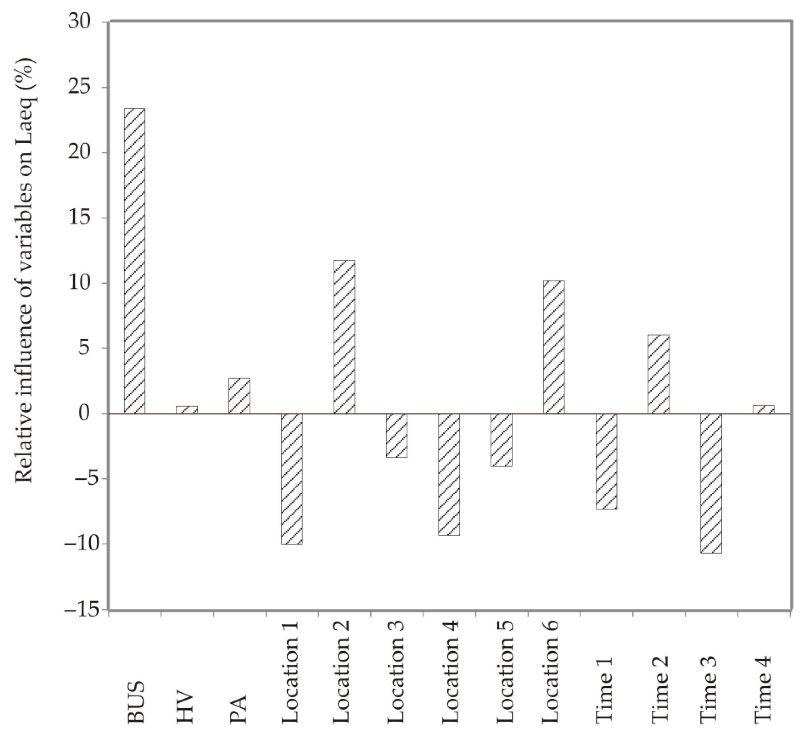
3.1.5. Global Sensitivity Analysis—Yoon’s Interpretation Method

In this section, the influence of input variables, used to build the ANN model on the relative importance of Laeq, is studied. According to Figure 8, BUS was the most influential parameter, with an approximately relative importance of 23.39%, while the influence of nighttime was negative, showing an importance of −10.68%. Futoska and Temerinska locations also showed a positive influence on Laeq, showing a relative importance of 11.75% and 10.18%. Jiménez-Uribe et al. [61] also revealed that the number of vehicles and the noise levels differed significantly according to the time of day and particular location. In addition, the noise levels were associated with the number of cars, buses and heavy vehicles.

4. Conclusions

As one of the main pollutants, in addition to hazardous gases, noise is a severe risk to people’s health, caused mainly by traffic in residential and business zones.

For this research, a total of five typical intersections in Novi Sad, Serbia, were selected, as well as one test intersection, which was used for model testing.

The measurement results show a high degree of correlation between noise intensity and the number of cars, as well as the number of buses and trucks. An increase in noise intensity that occurred during a heavier flow of buses and/or trucks was determined at almost every intersection.

Obtained non-linear models for forecast traffic noise levels gave high anticipation accuracy of the equivalent continuous sound level (Laeq), with R² values of 0.697, 0.703, 0.959 and 0.882, for two artificial neural networks and two random forest models, respectively. The current study suggests that RFR and ANN modelling can be successfully exploited for traffic noise level prediction. The incorporation of more input data can improve the efficacy of all tested models. This study has the potential to direct a new way to promising research related to traffic noise prediction.

The limitations of the obtained models are found in the fact that it is related exclusively to traffic flows, that is, the model does not consider noise pollution which may occur independently. Furthermore, the values of the noise reflecting from nearby objects were not precisely determined.

Further research on the dependency between traffic and noise should be conducted to determine other parameters that might be related to traffic flow and noise intensity.

References

1. World Health Organization; Regional Office for Europe. Environmental Noise Guidelines for the European Region. 2018. Available online: https://www.euro.who.int/en/publications/abstracts/environmental-noise-guidelines-for-the-european-region-2018 (accessed on 20 January 2021).
2. Boryaev, A.; Malygin, I.; Marusin, A. Areas of focus in ensuring the environmental safety of motor transport. Transp. Res. Procedia 2020, 50, 68–76. [Google Scholar] [CrossRef]
3. Wong, C.K.; Lee, Y.Y. The Effects of Signal System and Traffic Flow on the Sound Level. Appl. Sci. 2020, 10, 4454. [Google Scholar] [CrossRef]
4. Van Kempen, E.; Casas, M.; Pershagen, G.; Foraster, M. WHO environmental noise guidelines for the European region: A systematic review on environmental noise and cardiovascular and metabolic effects: A summary. Int. J. Environ. Res. Public Health 2018, 15, 379. [Google Scholar] [CrossRef] [PubMed]
5. Brink, M.; Stahel, W.A.; Basner, M. Determination of awakening probabilities in night time noise effects research. Somnol. Schlafforschung Schlafmed. 2009, 31, 236. [Google Scholar] [CrossRef]
6. Pirrera, S.; De Valck, E.; Cluydts, R. Nocturnal road traffic noise: A review on its assessment and consequences on sleep and health. Environ. Int. 2010, 36, 492–498. [Google Scholar] [CrossRef]
7. Münzel, T.; Schmidt, F.P.; Steven, S.; Herzog, J.; Daiber, A.; Sørensen, M. Environmental noise and the cardiovascular system. J. Am. Coll. Cardiol. 2018, 71, 688–697. [Google Scholar] [CrossRef]
8. Dutilleux, G.; Paviotti, M.; Backman, A.; Gergely, B.; McManus, B.; Bento Coelho, L.; Hinton, J.; Kephalopoulos, S.; Licitra, G.; Rasmussen, S.; et al. Good practice guide on noise exposure and potential health effects. In European Environmental Agency Technical Report, 1st ed.; Babisch, W., van den Berg, M., Eds.; Official Publications of the European Union: Luxembourg, 2010; pp. 1–40. [Google Scholar]
9. Ozdenerol, E.; Huang, Y.; Javadnejad, F.; Antipova, A. The impact of traffic noise on housing values. J. Real Estate Pract. Educ. 2015, 18, 35–53. [Google Scholar] [CrossRef]
10. Szopińska, K.; Krajewska, M.; Kwiecień, J. The Impact of Road Traffic Noise on Housing Prices-Case Study in Poland. Real Estate Manag. Valuat. 2020, 28, 21–36. [Google Scholar] [CrossRef]
11. Theebe, M.A. Planes, trains, and automobiles: The impact of traffic noise on house prices. J. Real Estate Finance Econ. 2004, 28, 209–234. [Google Scholar] [CrossRef]
12. UN Environment Programme. Noise, Blazes and Mismatches; UN Environment Programme: Nairobi, Kenya, 2022. [Google Scholar]
13. Khomenko, S.; Cirach, M.; Barrera-Gómez, J.; Pereira-Barboza, E.; Iungman, T.; Mueller, N.; Foraster, M.; Tonne, C.; Thondoo, M.; Jephcote, C.; et al. Impact of road traffic noise on annoyance and preventable mortality in European cities: A health impact assessment. Environ. Int. 2022, 162, 107160. [Google Scholar] [CrossRef]
14. Schomer, P.D. Criteria for assessment of noise annoyance. Noise Control Eng. J. 2005, 53, 125–137. [Google Scholar] [CrossRef]
15. Hood, R.A. Calculation of Road Traffic Noise. Appl. Acoust. 1987, 21, 139–146. [Google Scholar] [CrossRef]
16. Mishra, R.K.; Mishra, A.R.; Singh, A. Traffic noise analysis using RLS-90 model in urban city. In Proceedings of the INTER-NOISE and NOISE-CON Congress and Conference Proceedings, Madrid, Spain, 16–19 June 2019. [Google Scholar]
17. Noise, T. Nord 2000. New Nordic Prediction Method for Road Traffic Noise; SP Rapport 2001:10; DiVA: Uppsala, Sweden, 2001. [Google Scholar]
18. Tomic, J.Z. Application of Soft Computing Techniques in Traffic Noise Prediction. Ph.D. Thesis, University of Belgrade, Belgrade, Serbia, 2017. [Google Scholar]
19. Jandacka, D.; Decky, M.; Durcanska, D. Traffic Related Pollutants and Noise Emissions in the Vicinity of Different Types of Urban Crossroads. IOP Conf. Ser. Mater. Sci. Eng. 2019, 661, 012152. [Google Scholar] [CrossRef]
20. Van Blockland, G.J.; De Graff, D.F. Measures on Road Traffic Noise in the EU; Interest Group on Traffic Noise Abatement: Springfield, KY, USA, 2012; pp. 1–48. [Google Scholar]
21. Bühlmann, E.; Egger, S. Assessing the noise reduction potential of speed limit 30 km/h. In Proceedings of the INTER-NOISE 2017—46th International Congress on Noise Control Engineering, Hong Kong, China, 27–30 August 2017. [Google Scholar]
22. Institut za Bezbednosti i Sigurnost na Radu Doo. Monitoring buke u Životnoj Sredini (Environmental Noise Monitoring).pdf. 2018. Available online: http://www.ekourbapv.vojvodina.gov.rs/wp-content/uploads/2018/08/monitoring-buke-APV-SU2018-2.pdf (accessed on 1 September 2020).
23. “Urbanizam”, Public Enterprise, Saobraćajna Studija Grada Novog Sada sa Dinamikom Uređenja Saobraćaja (Traffic Study of the City of Novi Sad with the Dynamics of Traffic Organization); Нoстрам: Novi Sad, Serbia, 2009.
24. Dangel, U.; McDonagh, P.; Murphy, L. Traffic-condition Analysis using Publicly-Available Data Sets. 12th Inf. Technol. &Telecommunications Conf. 2013. Available online: http://hdl.handle.net/10344/3353 (accessed on 1 September 2020).
25. Official Journal of the European Communities. Directive 2002/49/EC of the European Parlament and of the Council. 2002. Available online: https://eur-lex.europa.eu/LexUriServ/LexUriServ.do?uri=OJ:L:2002:189:0012:0025:EN:PDF (accessed on 1 September 2020).
26. Official Journal of the European Communities. Recommendation 2003/613/EC concerning the Guidelines on the Revised Interim Computation Methods for Industrial Noise, Aircraft Noise, Road Traffic Noise and Railway Noise, and Related Emission Data. Available online: https://leap.unep.org/countries/eu/national-legislation/commission-recommendation-2003613ec-concerning-guidelines-revised (accessed on 20 January 2021).
27. ISO 1996-1:2016; Acoustics—Description, Measurement and Assessment of Environmental Noise—Part 1: Basic Quantities and Assessment Procedures. International Organization for Standardization: Geneva, Switzerland, 2016. Available online: https://www.iso.org/standard/59765.html (accessed on 1 September 2020).
28. Genaro, N.; Torija, A.; Ramos-Ridao, A.; Requena, I.; Ruiz, D.P.; Zamorano, M. A neural network based model for urban noise prediction. J. Acous. Soc. Am. 2010, 128, 1738–1746. [Google Scholar] [CrossRef] [PubMed]
29. Garg, N.; Mangal, S.K.; Saini, P.K.; Dhiman, P.; Maji, S. Comparison of ANN and Analytical Models in Traffic Noise Modeling and Predictions. Acoust. Aust. 2015, 43, 179–189. [Google Scholar] [CrossRef]
30. Tiwari, G.; Fazio, J.; Gaurav, S. Traffic planning for nonhomogeneous traffic. Sadhana 2007, 32, 309–328. [Google Scholar] [CrossRef]
31. Givargis, S.; Karimi, H. A basic neural traffic noise prediction model for Tehran’s roads. J. Environ. Manag. 2010, 91, 2529–2534. [Google Scholar] [CrossRef]
32. Parabat, K.; Nagarnaik, P.B. Assessment and ANN modeling of noise levels at major road intersections in an Indian intermediate city. J. Res. Sci. Comput. Eng. 2007, 4, 39–49. Available online: http://www.ejournals.ph/form/cite.php?id=2168 (accessed on 10 May 2022). [CrossRef]
33. Torija, A.J.; Rúiz, D.P.; Ramos-Ridao, A.F. Use of backpropagation neural networks to predict both level and temporal spectral composition of sound pressure in urban sound environments. Build. Environ. 2012, 52, 45–56. [Google Scholar] [CrossRef]
34. Mansourkhaki, A.; Berangi, M.; Haghiri, M.; Haghani, M. A neural network noise prediction model for Tehran urban roads. J. Environ. Eng. Landsc. 2018, 26, 88–97. [Google Scholar] [CrossRef]
35. Liu, Y.; Oiamo, T.; Rainham, D.; Chen, H.; Hatzopoulou, M.; Brook, J.R.; Davies, H.; Goudreau, S.; Smargiassi, A. Integrating random forests and propagation models for high-resolution noise mapping. Environ. Res. 2021, 195, 110905. [Google Scholar] [CrossRef] [PubMed]
36. Staab, J.; Schady, A.; Weigand, M.; Lakes, T.; Taubenböck, H. Predicting traffic noise using land-use regression—A scalable approach. J. Expo. Sci. Environ. Epidemiol. 2022, 32, 232–243. [Google Scholar] [CrossRef] [PubMed]
37. Adulaimi, A.A.A.; Pradhan, B.; Chakraborty, S.; Alamri, A. Traffic Noise Modelling Using Land Use Regression Model Based on Machine Learning, Statistical Regression and GIS. Energies 2021, 14, 5095. [Google Scholar] [CrossRef]
38. The Ministry of Environmental Protection, Government of Serbia. Rulebook on Noise Measurement Methods, Content and Scope of the Noise Measurement Report. Official Gazette of the Republic of Serbia, No. 72/10. Available online: https://rspdf.info/%D0%B4%D0%BE%D0%BA%D1%83%D0%BC%D0%B5%D0%BD%D1%82/2e2ddc6/pravilnik-o-metodama-meren%D1%98a-buke-sadr%C5%BEini-i-obimu--putevi-srbije (accessed on 1 September 2020).
39. The Ministry of Environmental Protection, Government of Serbia. Regulation on Noise Indicators, Limit Values, Methods for Evaluation of Noise Indicators, Harassment and Harmful Effects of Environmental Noise. 2010. Available online: https://www.putevi-srbije.rs/images/pdf/regulativa/uredba_o_indikatorima_buke_GV_metodama_za_ocenjivanje_indikatora_buke.pdf (accessed on 1 September 2020).
40. Saad Ahmad Abo-Qudais, A.A. Effect of distance from road intersection on developed traffic noise levels. Can. J. Civ. Eng. 2011, 31, 533–538. [Google Scholar] [CrossRef]
41. European Parliament, Council of the European Union. Regulation (EU) No 540/2014. 2014. Available online: https://eur-lex.europa.eu/eli/reg/2014/540/oj (accessed on 1 September 2020).
42. Aguilera, I.; Foraster, M.; Basagaña, X.; Corradi, E.; Deltell, A.; Morelli, X.; Phuleria, H.C.; Ragettli, M.S.; Rivera, M.; Thomasson, A.; et al. Application of land use regression modelling to assess the spatial distribution of road traffic noise in three European cities. J. Expo. Sci. Environ. Epidemiol. 2015, 25, 97–105. [Google Scholar] [CrossRef]
43. Ryan, P.H.; LeMasters, G.K. A review of land-use regression models for characterizing intraurban air pollution exposure. Inhal. Toxicol. 2007, 19, 127–133. [Google Scholar] [CrossRef]
44. Kollo, T.; von Rosen, D. Advanced Multivariate Statistics with Matrices. In Mathematics and Its Applications, 1st ed.; Hazewinkel, M., Ed.; Springer: Dordrecht, The Netherlands, 2005; Volume 579, pp. 1–485. [Google Scholar]
45. Pezo, L.; Ćurčić, B.L.; Filipović, V.S.; Nićetin, M.R.; Koprivica, G.B.; Mišljenović, N.M.; Lević, L.B. Artificial neural network model of pork meat cubes osmotic dehydration. Hem. Ind. 2013, 67, 465–475. [Google Scholar] [CrossRef]
46. Hosseini, A.S.; Hajikarimi, P.; Gandomi, M.; Nejad, F.M.; Gandomi, A.H. Optimized machine learning approaches for the prediction of viscoelastic behavior of modified asphalt binders. Constr. Build. Mater. 2021, 299, 124264. [Google Scholar] [CrossRef]
47. Shukla, V.; Khandekar, P.; Khaparde, A. Noise estimation in 2D MRI using DWT coefficients and optimized neural network. Biomed. Signal Process. Control 2022, 71, 103225. [Google Scholar] [CrossRef]
48. Seshia, S.A.; Sadigh, D.; Sastry, S.S. Toward verified artificial intelligence. Commun. ACM 2022, 65, 46–55. [Google Scholar] [CrossRef]
49. Yoon, Y.; Swales, G.; Margavio, T.M. Comparison of Discriminant Analysis versus Artificial Neural Networks. J. Oper. Res. Soc. 2017, 44, 51–60. [Google Scholar] [CrossRef]
50. Breiman, L. Random forests. Mach. Learn. 2001, 45, 5–32. [Google Scholar] [CrossRef]
51. Liu, Y.; Goudreau, S.; Oiamo, T.; Rainham, D.; Hatzopoulou, M.; Chen, H.; Davies, H.; Tremblay, M.; Johnson, J.; Bockstael, A.; et al. Comparison of land use regression and random forests models on estimating noise levels in five Canadian cities. Environ. Pollut. 2020, 256, 113367. [Google Scholar] [CrossRef]
52. Rajković, D.; Marjanović Jeromela, A.; Pezo, L.; Lončar, B.; Zanetti, F.; Monti, A.; Kondić Špika, A. Yield and Quality Prediction of Winter Rapeseed—Artificial Neural Network and Random Forest Models. Agronomy 2022, 12, 58. [Google Scholar] [CrossRef]
53. Montgomery, D.C. Design and Analysis of Experiments, 2nd ed.; John Wiley and Sons: Hoboken, NJ, USA, 1984; pp. 1–556. [Google Scholar]
54. Debnath, A.; Singh, P.K.; Banerjee, S. Vehicular traffic noise modelling of urban area—A contouring and artificial neural network based approach. Environ. Sci. Pollut. Res. 2022, 29, 39948–39972. [Google Scholar] [CrossRef]
55. Kumar, P.; Nigam, S.P.; Kumar, N. Vehicular traffic noise modeling using artificial neural network approach. Transp. Res. C Emerg. Technol. 2014, 40, 111–122. [Google Scholar] [CrossRef]
56. Nourani, V.; Gökçekuş, H.; Umar, I.K.; Najafi, H. An emotional artificial neural network for prediction of vehicular traffic noise. Sci. Total Environ. 2020, 707, 136134. [Google Scholar] [CrossRef]
57. Cammarata, G.; Cavalier, S.; Fichera, A. A neural network architecture for noise prediction. Neural Netw. 1995, 8, 963–973. [Google Scholar] [CrossRef]
58. Hamoda, M.F. Modeling of construction noise for environmental impact assessment. J. Construct. Dev. Ctries. 2008, 13, 79–89. [Google Scholar]
59. Erbay, Z.; Icier, F. Optimization of hot air drying of olive leaves using response surface methodology. J. Food Eng. 2009, 91, 533–541. [Google Scholar] [CrossRef]
60. Turanyi, T.; Tomlin, A.S. Analysis of Kinetics Reaction Mechanisms, 1st ed.; Springer: Berlin/Heidelberg, Germany, 2014; pp. 1–363. [Google Scholar]
61. Jiménez-Uribe, D.A.; Daniels, D.; Fleming, Z.L.; Vélez-Pereira, A.M. Road Traffic Noise on the Santa Marta City Tourist Route. Appl. Sci. 2021, 11, 7196. [Google Scholar] [CrossRef]
Figure 1. The intersections selected for the research: R1—Boulevard Oslobođenja–Novosadskog sajma street, R2—Boulevard Kralja Petra I–Rumenačka street, R3—Boulevard Cara Lazara–Boulevard Cara Dušana, R4—Boulevard Cara Lazara–Boulevard oslobođenja, R5—Partizanska street–Temerinska street (https://www.google.com/maps/search/novi+sad+street+view/@45.2671726,19.8416325,18z?hl=en, accessed on 19 June 2019).
Sustainability 14 12443 g001
Figure 2. Meteorological parameters during the period of measurement (https://www.meteoblue.com/sr/vreme/historyclimate/weatherarchive/novi-sad_%d0%a1%d1%80%d0%b1%d0%b8%d1%98%d0%b0_3194360, accessed on 1 June 2019).
Sustainability 14 12443 g002
Figure 3. Noise measurement positions at intersection: IVa position—5 m from intersection and IVb position—50 m from intersection.
Sustainability 14 12443 g003
Figure 4. Results of measurement at f six intersection: (a) number of passenger cars in a 15-min interval, (b) Laeq and number of heavy vehicles in a 15-min interval.
Sustainability 14 12443 g004
Figure 5. Comparison between experimentally obtained and model-predicted values of noise level based on the traffic volume at intersections for (a) ANN1 model, (b) RFR1 model, (c) ANN2 model, (d) RFR2 model.
Sustainability 14 12443 g005
Figure 6. Comparison between experimentally obtained and model-predicted values of calculated outputs for Laeq Gras location for (a) ANN1 model, (b) RFR1 model, (c) ANN2 model, (d) RFR2 model.
Sustainability 14 12443 g006
Figure 7. Spatial distribution of average Laeq value during the day, related to the investigated locations in Novi Sad, based on the ANN1 model.
Sustainability 14 12443 g007
Figure 8. The relative importance of the variables on Laeq, determined using Yoon’s interpretation method.
Sustainability 14 12443 g008