Article

Analysing the Recent Dynamics of Agricultural Sustainability in Portugal Using a Compromise Programming Approach

by
António Xavier
1,*,
Maria de Belém Costa Freitas
2,
Rui Fragoso
3 and
Maria do Socorro Rosário
4
1
CEFAGE (Center for Advanced Studies in Management and Economics), University of Évora, Largo dos Colegiais, 7000-803 Évora, Portugal
2
Sciences and Technology Faculty, MED—Mediterranean Institute for Agriculture, Environment and Development, University of Algarve, Gambelas Campus, 8005-139 Faro, Portugal
3
CEFAGE-UE (Center for Advanced Studies in Management and Economics), Management Department, Universidade de Évora, N° 2, Apt. 95, 7002-554 Evora, Portugal
4
Direção de Serviços de Estatística, GPP (Gabinete de Planeamento e Políticas), Praça do Comércio, 1149-010 Lisbon, Portugal
*
Author to whom correspondence should be addressed.
Sustainability 2022, 14(19), 12512; https://doi.org/10.3390/su141912512
Submission received: 2 August 2022 / Revised: 19 September 2022 / Accepted: 26 September 2022 / Published: 30 September 2022
(This article belongs to the Section Sustainable Agriculture)

Abstract

:
Society recognises the importance of agriculture to supply goods, which are essential for human survival and well-being. Sustainable agriculture is an important goal since resources need to be preserved for future generations. The recent agricultural policy orientations towards environmental concerns have also had consequences for Portuguese agriculture. The information provided by the 2019 Agricultural Census offers an opportunity to analyse the recent dynamics and establish rankings of municipalities related to agricultural sustainability. Sustainability in agriculture can be studied using different types of indicators, but its quantification and aggregation into an index is still difficult. This paper proposes an approach based on compromise programming to analyse sustainability considering the dynamics between the 2009 and 2019 Agricultural Census. This approach has three main steps: in the first one, the indicators are selected and a HJ-Biplot and Cluster analysis are carried out to identify groups of municipalities and general dynamics; in the second step, the weights of indicators are defined, and a novel compromise programming model is implemented to define the rankings of sustainability for each year; finally, in the third step, the spatial dynamics of the sustainability rankings are analysed and classified into the clusters of municipalities previously created. The analysis was implemented using data from the 308 Portuguese municipalities for 12 individual indicators encompassing the several dimensions of sustainability. The results were promising since the approach allowed for the identification of the main dynamics and tendencies regarding sustainability.

1. Introduction

Agriculture supplies goods that are essential for human survival and well-being. In that scope, sustainable agriculture is an important goal since resources need to be preserved for future generations. According to the Brundtland Report, sustainability may be defined as ‘the development that meets the needs of the present without compromising the ability of future generations to meet their own needs.’ It is a complex concept, which integrates economic, social, and environmental dimensions [1].
The recent agricultural policy orientations towards environmental concerns have also had consequences for Portuguese agriculture [2,3]. To analyse agricultural sustainability, the information provided by the 2019 Agricultural Census offers an opportunity to study the recent dynamics and establish rankings of municipalities related to agricultural sustainability.
In that scope, composite indicators are very useful in spite of the aggregation of simple indicators in a single composite index still being difficult. There are several approaches and the OECD [4] presents several aggregation methods: additive aggregation, geometric aggregation, and the non-compensatory multi-criteria approach (MCA). Gómez-Limon and Sanchez-Fernandez [5], focusing particularly on agriculture, also present an assessment of several composite indicator approaches. Multicriteria decision analysis (MCDA) techniques may be of great importance for creating composite indicators and allowing ranking analysis [6,7].
Among MCDA techniques, we highlight two that allow for the creation of composite indicators and ranking analyses: extended goal programming (EGP) and compromise programming (CP).
Regarding EGP, several studies analysed sustainability [1,8,9,10,11,12]. These studies have focused on the sustainability of forest management [8], sustainability rankings of European wood manufacturing industries [9], optimal harvest scheduling in Eucalyptus plantations under a sustainability perspective [10], sustainability and the causes responsible for the level of sustainability [11], sustainability ranking of forest plantations, triple bottom line solutions of sustainability [12], and the analysis of agricultural sustainability at the municipal level [1].
From these mentioned studies, we highlighted [1], which developed a methodology for evaluating agricultural sustainability considering national goals and utilising EGP. These authours also proposed a general approach utilising entropy to perfect the ranking in cases of similar index values. Nevertheless, they focused on the 2009 National Agricultural Census using EGP and considered other goals that are used in this analysis.
For compromise programming there are less studies [3,13]. The main subjects analysed were the sustainability of water use in Portugal [3] and the paper industry in different EU countries [13]. Costa Freitas et al. [3] continued the previous study [1] and presented a novel compromise programming approach by using entropy, which allowed perfecting of the results and solving the problem of similar indexes corresponding to different situations. This approach offers great potential to define rankings and needs to be implemented to define agricultural sustainability in a dynamic way.
For the analysis of rankings of sustainability, multivariate techniques also may be used. One of them is the HJ-Biplot [14], which have a variety of studies [15,16,16,17,18,19] and may be combined with cluster analyses [15,16]. Xavier and Costa Freitas [16] showed the great potential of this approach to analyse agricultural dynamics and identify trends.
Therefore, the objective of this paper is to analyse the recent dynamics of agricultural sustainability in Portuguese municipalities, considering the last two agricultural censuses (2009 and 2019). To achieve this objective, a novel approach is proposed, which uses an HJ-Biplot, cluster analysis, and compromise programming to create a composite indicator and define sustainability rankings, whose geographical distribution is analysed.
This article provides several contributions to the literature. First, it presents a novel compromise programming approach for a ranking analysis of agricultural sustainability, which has several advantages: it allows for the definition of sustainability rankings for a large number of decision units and the solving of situations of equal ranking position. Secondly, the use of an HJ-Biplot analysis allows for the definition of homogeneous groups in municipalities and the analysis of the relations among variables that are considered for the building of the composite index. Finally, an analysis of the geographical distribution of the results allows for an operational application of the results. Therefore, the article gives insights about agricultural sustainability rankings, spatial patterns, and dynamics, which might allow for a better policy design and implementation.
The remainder of the article is organised as follows: in Section 2, the methodological approach is presented; in Section 3, the empirical implementation is analysed; in Section 4, the results presented are discussed; finally, Section 5 presents the main conclusions.

2. Materials and Methods

2.1. The Methodological Approach

The proposed approach is inspired by the works of [1,3,13] and follows several works, which implemented an HJ-Biplot and cluster analysis [15,16,19,20,21]. Figure 1 summarizes the methodological steps of the approach.
This approach is developed into three main steps, as follows:
1° step—Selection of agricultural indicators and implementation of an HJ-Biplot and Cluster analysis to create typologies and, hence, provide a better analysis of the rankings.
2° step—The preferential criteria weights are derived from pairwise comparisons by using EGP [1,3,22,23] and compromise programming to calculate the composite indicator and define the rankings of agricultural sustainability. This step ends up applying an entropy approach to perfect the rankings [3].
3° step—A geographic information system (GIS) is used to analyse the rankings and its dynamics between the two censuses (2009 and 2019). This analysis of the groups of the municipalities resulting from the cluster analysis allows for a better understanding of the underlying typologies and their main explicative indicators.

2.2. The HJ-Biplot and Cluster Analysis

A biplot is a graphical representation of multivariate data. The concept of a biplot means that in the graph that represents the elements of a data matrix, there are two types of markers: markers (vectors) representing individuals and markers (vectors) representing variables [24]. The axes are not perpendicular and allow for the projection of an N-dimensional representation with a minimum loss of information that adds an interpretative meaning.
According to [24], any matrix of rank two can be displayed graphically as a biplot, which consists of a vector for each row and a vector for each column, chosen such that any element of the matrix is exactly the inner product of the vectors corresponding to its row and its column. If a matrix is of a higher rank, one may display it as a biplot of a rank two matrix, which approximates the original matrix. The rank of a matrix is the number if row or column vectors are needed to generate the rows or columns of a matrix through linear combinations. This algebraic concept is equivalent to the dimensionality of a matrix. A rank two matrix is a matrix that results from multiplying a matrix with 2 columns by a matrix with 2 rows.
The biplot provides a data analysis tool that allows for the visual representation of large data matrices [24]. The initial matrix can be written according to the singular value decomposition (for more details see [16]). According to [24], there are different types of biplots: JK or RMP is called a row metric preserving biplot; GH or CMP is called a column metric preserving biplot and this display preserves distances between the columns, leading to a high quality for the variables; SQRT (symmetric biplot) is a compromise situation [16].
It was demonstrated that the HJ-Biplot was able to produce better results than the previous classic biplot methods [14] since this method achieves an optimum representation quality for both rows and columns, because they are represented in the same system [14,17,18].
A representation HJ-Biplot for a data matrix X containing the units is defined as a graphical representation by multivariate markers j1, j2, … jn for lines and h1, h2, …, hn for the columns of X, selected so that both markers may overlap in the same reference system with high quality representation. The lines are represented by dots and the columns by vectors [14]. Thus, the HJ-Biplot is based on singular value decomposition (SVD) of the data matrix, and any matrix may be factored in as the product of three matrices, such that [15,16]:
X n x p = U n x r Ʌ r x r V r x p   with   U U = V V = I r
where U n x r is the matrix of eigenvectors of XX’; V r x p is the matrix of eigenvectors of X’X; Ʌ r x r is a diagonal matrix of λ 1 λ 2 λ 3 λ r corresponding to the r eigenvalues of XX’ or X’X.
The elements of X n x p are given by:
x i j = k = 1 r λ k u k v j k i = 1 , 2 , , n j = 1 , 2 , p .  
For details of the HJ-Biplot model results, see, for instance, [15,16,17,18]. The interpretation of the results [15,16,25] of a HJ-Biplot representation is as follows:
-
Gabriel [24] shows that the cosine of the angle between the vectors representing the variables in a biplot is the correlation coefficients between the respective variables. This means that if two attributes are positively correlated, vectors that represent the variables form acute angles, and if two attributes are inversely correlated, the vectors that represent the variables form obtuse angles. If an attribute does not have any relationship with another attribute, the markers that represent the biplot graphic form a right angle and the correlation between the attributes is null.
-
The distance between row points is interpreted as similarity, and if a row point is close to a column point (variable), this is interpreted as preponderance [17].
-
The closer the direction of a variable is to a representative point of an individual and the greater spacing of the individual in relation to the centre, the higher the prevalence or importance of this variable in explaining the results obtained by an individual.
-
Attributes with higher variance are represented by longer vectors.
-
The smaller the angle between the vectors defined by the centre of the biplot and markers of an individual and of a variable, the greater the affinity between this indivial and this variable, in the sense described.
A cluster analysis may then be applied to the resulting HJ-Biplot coordinates to create a homogeneous group of decision units [16].

2.3. Sustainability Indicators’ Weights

To define the weights assigned to each indicator, several studies used group decision methods. One of the most used is the analytical hierarchical process (AHP), which uses pairwise comparisons. This is a good approach to define the relative importance of several criteria [22,26]. These pairwise comparisons can be aggregated by the geometric mean method or the weighted arithmetic mean method. Other solutions to deal with pairwise comparisons use an Extended Goal Programming approach developed by [22] and implemented by [1,3,23,27].
This approach has several advantages: (1) It allows for the handling of situations without satisfactory conditions regarding reciprocity and consistency; (2) it has a low computational burden; (3) it considers the analysis of the majority and minority consensus [1,3]. For the complete formulation, please see [1,3,23].

2.4. Ranking Analysis Definition

The first step in implementing the ranking analysis is the normalisation of each indicator Ric regarding each criterion i and unit c since they are measured in different units:
R ¯ i c = 1 R i * R i c R i * R * i = R i c R * i R i * R * i i 1 , 2 , , I   a n d   c 1 , 2 , C
where R i * is the best value of the ith indicator and R i * is the worst value achieved by the ith indicator. Thus, the matrix of R ¯ i c elements is a i × c matrix of normalized outcomes.
After the parameters Ric have been normalised, a binary compromise programming approach may be implemented, which allows for an iterative ranking construction, considering the trade-off among metrics L1 and L∞ [13]. In this case, the model is run n times, corresponding to the number of c geographical units considered. Alternatively, an aggregation of the model is proposed, according to [1,3], allowing the simultaneous solving for all c units, as follows:
M i n C I = c = 1 C C I c
C I c = 1 λ D c + λ i = 1 I α i c 1 R ¯ i c c 1 , 2 , , C λ 0 , 1
α i c ( 1 R ¯ i c ) D c   i 1 , 2 , , I   and   c 1 , 2 , C
where CIc represents the composite indicator of sustainability, which defines the ranking position of territorial unit c; αic are the weights of the i criteria in territorial unit c; and Dc is the maximum deviation for the i criteria in territorial unit c.
Equations (4) and (5) allow the minimisation of the aggregate objective function that minimises the unwanted deviation variables (highest aggregated sustainability) or the maximum deviation. For λ = 1, the model provides the solution with the maximum aggregate achievement and for λ = 0, it provides the solution with the most balanced achievement. For intermediate values of λ, compromise solutions can be achieved. Equation (6) calculates the maximum deviation D. Final ordering may be done using simple Microsoft Excel functions according to [1].
In certain situations, the previous compromise programming model can give a solution where there is more than one decision unit with the same value of CI in the ranking being ordered arbitrarily. References [1,3] proposed an entropy approach to deal with these issues in which the result is always a unique solution. Due to its advantages, this procedure was also implemented in this paper.
To implement this method, an alternative set of probabilities pric referring to the weight of deviation regarding the ideal (1 − R ¯ i c ) was created, such as:
p r i c = α i c 1 R ¯ i c i = 1 I α i c 1 R ¯ i c   a n d   i = 1 I p r i c = 1
According to the concept of normalised entropy, Dc can be replaced by the information index IDc:
I D c = 1 i = 1 I p r i c l n p r i c ln I
Then, the results of the previous compromise programming model can be used to compute the following expression of the composite indicator CIc, which allows unique solutions as follows [3]:
C I c = 1 λ I D c + λ i = 1 I α i c 1 R ¯ i c   c 1 , 2 , , C  

2.5. Empirical Implementation

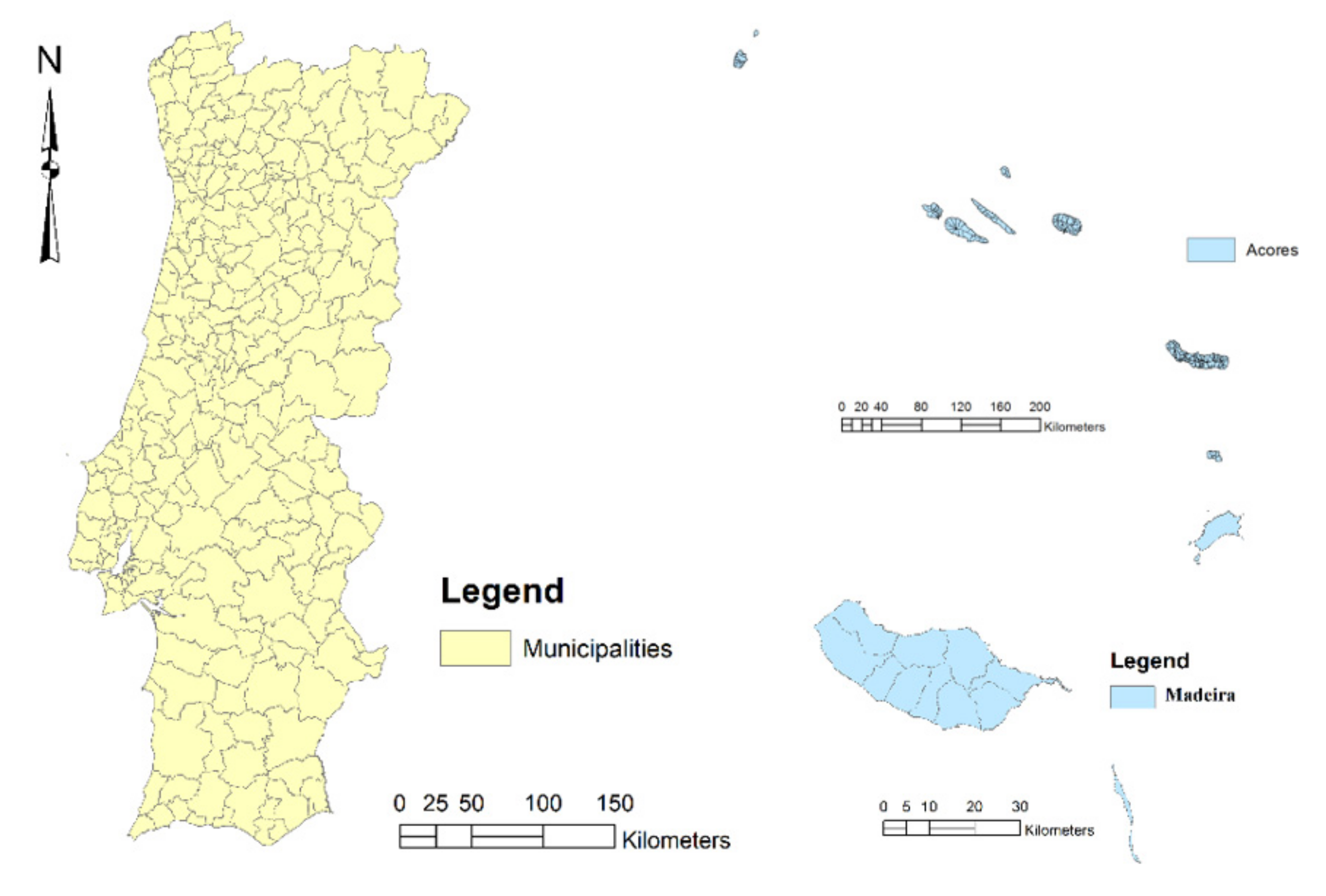
Figure 2 depicts the study area, which comprises the 308 municipalities of Portugal, including the insular territories (Azores and Madeira). The HJ-Biplot and the ranking analysis was implemented in these areas, but the spatial analysis of the results focused only on Portugal Mainland.
To implement this study, a screening of the data sources was done. The main data are the indicators collected by the National Statistics Institute (INE), namely from the National Agricultural Censuses of 2009 and 2019. The selected indicators for implementing the approach are presented in Table 1. We follow the agricultural sustainability indicators proposed by [1], adapting 10 indicators for this study among a set of 12. Ref. [1] selected the indicators following the recommendations of a panel of experts and the available information in the 2009 agricultural census. Note that [28] identified 17 possible indicators regarding the economic, social, and environmental dimensions, which, after expert analysis, were reduced to 12, that is, 4 in each sustainability dimension as in [1].
Our study focused on variables that are common in both censuses (2009 and 2019), and, hence, two indicators had to be different from those used in [1]. The percentage of farms with organic farming (AGRBIO) and the percentage of agricultural land in which manure was used (ESTR) replaced the following indicators, for which the 2019 census does not provide information: “Proportion of farms that have watertight storage facilities of effluents”; “Proportion of farms that burn the vegetal residuals without having another use for them.”
The indexes used were normalised according to their nature: less is better or more is better. Therefore, an increase in the normalised index will always mean a better result.
For the preferential criteria weights, we adapted the ones proposed by [1]. This study used an EGP model to derive a consensus from a set of experts, which includes university professors, officials from the Regional Office of Agriculture, technicians from the Planning and Policy Office of the Agricultural Ministry and researchers. These authours used the majority consensus to define the simple indicators’ weights. Regarding the two new indicators mentioned before, we used the same weights provided by [1] for the environmental indicators.
For the compromise programming model, the municipalities of Lisbon, Porto, and São João da Madeira were not considered in the ranking since they are atypical situations related to the fact that the legal registration of farms is there, but they are located in other municipalities.
In the definition of the groups of municipalities, we used the Biplot coordinates to apply a hierarchical cluster analysis method. The Euclidean distances were used as a dissimilarity index and for the linkage method, we considered the Ward’s method.
The application of the HJ-Biplot and cluster analysis were made using the Multbiplot software developed by [29]. To implement the proposed compromise programming model, a General Algebraic Modelling System (GAMS) code was developed. The final results were analysed geographically using ArcGIS 10.4.

3. Results

3.1. HJ-Biplot and Cluster Analysis

The results of the HJ-Biplot are presented as follows. In HJ-Biplot analysis, two axes with 47.97% of the accumulated inertia were retained. The relative contributions of the factor to the element are presented in Table 2. They allow for the determination of part of the variability of each variable that is explained by the factor. The axis where it is best represented is highlighted in bold for each variable.
The first axis is highly correlated with total standard output per farm (VPPEXP), proportion of farms with other revenue sources than agriculture (PATNGR), share of permanent hired labour (MNFAM), gender inequality (IGENEDIR), farmers’ education and training (EDAGR), and agricultural land with manure fertilisation (ESTR). Therefore, it presents the factors regarding economic and social sustainability without a focus on agricultural land. The second axis is correlated with standard output per hectare (VPP/SAU), aging of farmers (PR65), agricultural system intensity (ICULTHPES), livestock unit per utilised agricultural land (CNSAU) and farms with organic farming (AGRBIO). It represents agricultural land sustainability. Figure 3 presents the HJ-Biplot bidimensional representation.
Upon the analysis of Figure 3, we may identify the relationship among variables. Creation of agricultural employment (MNFAM) and total standard output per farm (VPPEXP) seem to be highly correlated. The same is applied to agricultural land with manure fertilisation (ESTR) and standard output per hectare of utilised agricultural land (VPP/SAU), but also agricultural system intensity (ICULTHPES) and livestock units per utilised agricultural land (CN/SAU).
We may also identify inverse correlations among several variables. Here we highlight that agricultural land with manure fertilisation (ESTR) is inversely correlated with livestock units per utilised agricultural land (CN/SAU), agricultural system intensity (ICULTHPES), proportion of farms with other revenue sources than agriculture (PATNGR) and farms with organic farming (AGRBIO). Gender inequality (IGENEDIR) is inversely correlated with share of permanent hired labour (MNFAM) and total standard output per farm (VPPEXP).
The following groups of municipalities were also identified according to how they tend to be more oriented to a certain set of sustainability indicators:
Group 1—Municipalities oriented to aging of farmers (PR65) and standard output per hectare (VPP/SAU), which are more associated with social and economic sustainability.
Group 2—Muncipalities with mixed sustainability, that is, municipalities that have some orientation to farmers’ education and training (EDAGR), share of permanent hired labour (MNFAM), and standard Output per farm (VPPEXP).
Group 3—Municipalities clearly oriented to farmers’ education and training (EDAGR), share of permanent hired labour (MNFAM), and total standard output per farm (VPPEXP).
Group 4—Municipalities oriented to agricultural land with manure fertilisation (ESTR) and agricultural area evolution (TABAND).
Group 5—Muncipalities with mixed orientations namely oriented to gender inequality (IGENEDIR) and agricultural system intensity (ICULTHPES).
The spatial dynamics of the clusters of municipalities is presented in Figure 4. In 2009, group 5 is mostly dominant in the centre and north of the Portugal mainland, but also in part of the Algarve Region. Group 2 is limited to part of the centre, littoral north, and some municipalities in the south and Group 3 mainly integrates municipalities of the Alentejo Region. The other groups seem to have a lower territorial expression: group 1 is mainly in the littoral centre and north and group 4 is in the centre and north of Portugal.
Regarding dynamics, we must highlight that group 3 and 5 seem to gain territorial expression from 2009 to 2019, while group 1, 2, and 4 clearly lost territorial expression in the Portugal mainland.

3.2. Rankings of Sustainability

The proposed compromise programming model allowed for the obtaining of a complete set of indexes and rankings for the years 2009 and 2019, which were then improved using the entropy approach presented before. As mentioned, the weights assigned the α_ic vector for each sustainability indicator were the ones used by [1], which reflect the majority consensus.
Table 3 and Table 4 present the 10 best placed municipalities. As stated before, λ = 1 situation maximises the aggregated sustainability and λ = 0, the most balanced sustainability, and intermediate solutions may be obtained. In 2009, Barrancos presented the best results for all scenarios, except for λ = 0, where the best placed municipality was Alcochete. The second place spot is occupied by Benavente for λ = 1 to λ = 0.2. Third place is occupied by Vila do Conde from λ = 1 to λ = 0.5; then by Alcochete from λ = 0.3 to λ = 0.2 and by Alpiarça from λ = 1 to λ = 0. In 2019, Alcochete presented the best results for all scenarios, except for λ = 0, where it was replaced by Cartaxo. It is then followed by Monforte and Alcácer do Sal for λ = 1 to λ = 0.2, which was only replaced in λ = 0 by Lagos and Caldas da Rainha. Considering the two sets of years, we must highlight that Barrancos had a decrease in agricultural sustainability, while Alcochete seems to have improved its aggregated sustainability.

3.3. Spatial Patterns and Dynamics

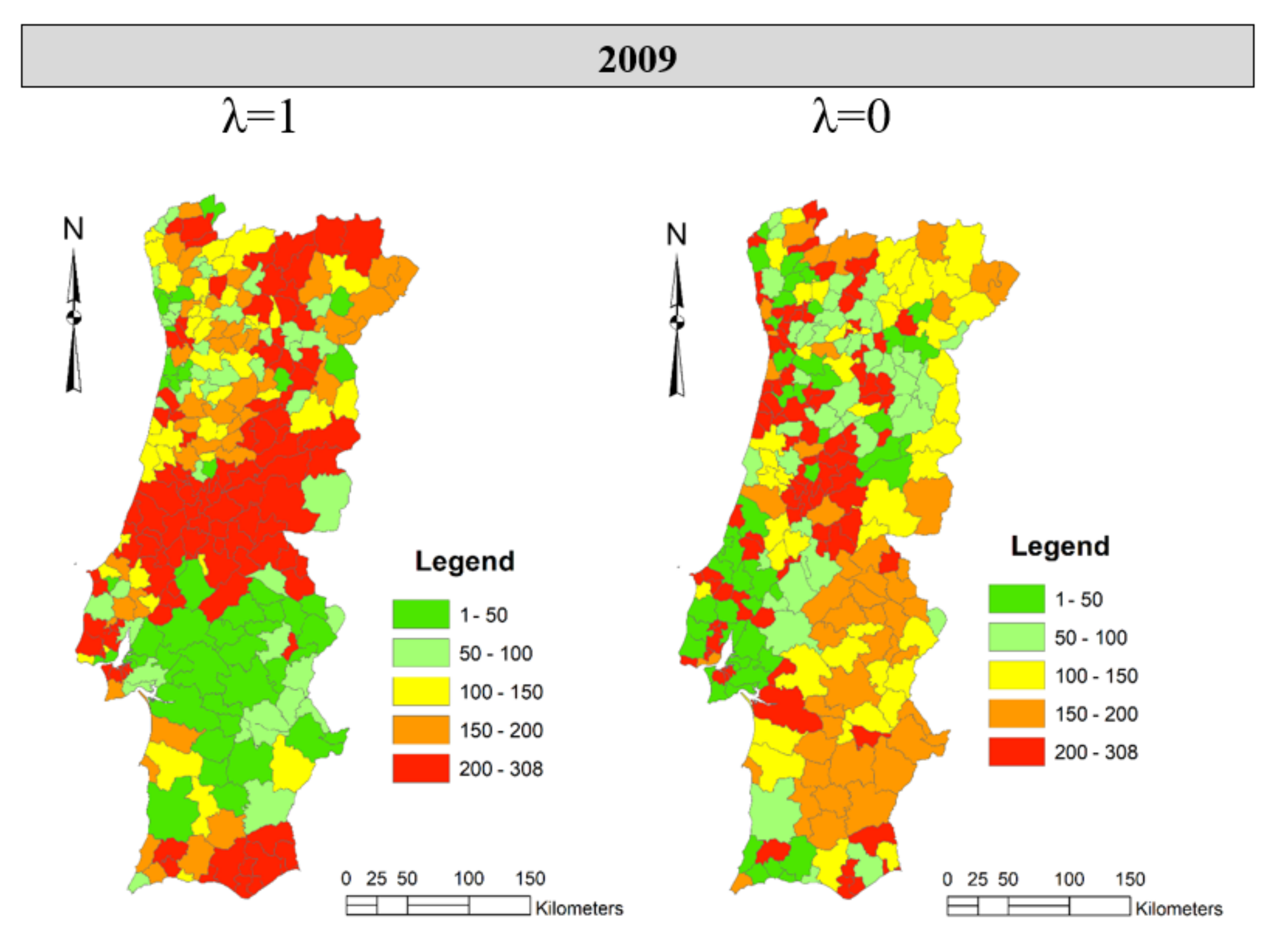
The results from the compromise programming model were inserted in a geographical information system (GIS) to analyse the patterns and dynamics. Figure 5 and Figure 6 present some examples of maps for λ = 1, “the best aggregated sustainability”, and λ = 0, “the most balanced sustainability”, for 2009 and 2019.
In 2009 for λ = 1 (Figure 5), the municipalities within the first 50 places tend to be mostly in the Alentejo Region. The municipalities with lower ranking positions are situated in the centre and northern areas, but also in part of the Algarve Region. For λ = 0, the best-positioned 50 municipalities have a different pattern. They seem to be more located in the region of Lisbon and Ribatejo, while there are some dispersed in the Algarve Region, centre, and north. Regarding the municipalities with positions lower than 200th, they are mostly concentrated in the central region.
In 2019 for λ = 1 (Figure 6), the municipalities within the first 50 places tend to be mostly at the Alentejo Region, while the municipalities with lower ranking positions are located in the centre and northern areas, but also in part of the Algarve Region, therefore, following the same tendencies as 2009. For λ = 0, the best-positioned 50 municipalities seem to be more located in the regions of Lisbon and Ribatejo, centre north, and part of the Algarve. Regarding the municipalities with positions lower than 200th, they are mostly concentrated in the inner regions of Alentejo and the centre.
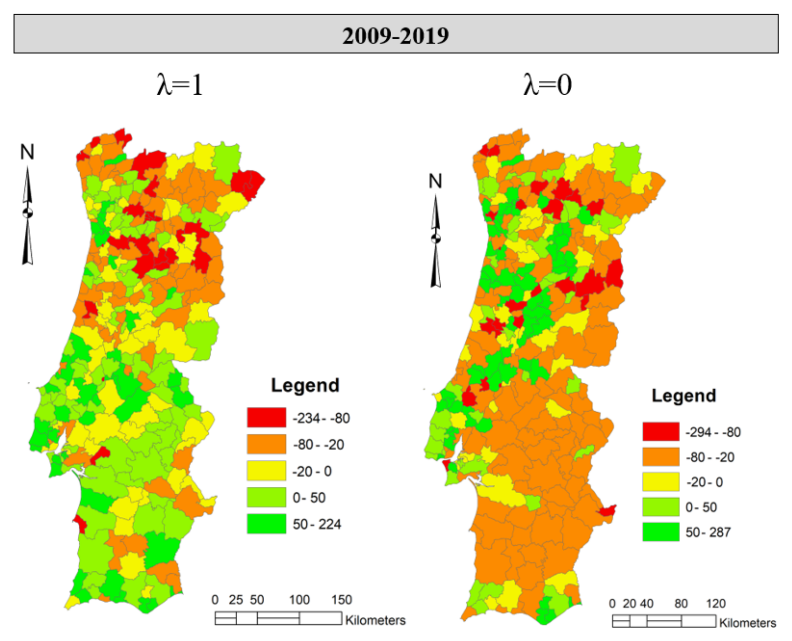
The combination of the two previous maps enabled the identification of the municipalities’ position and general situation each year. Therefore, a map of the variations in sustainability ranking positions was built to depict their dynamics (Figure 7).
For λ = 1, the municipalities with positive dynamics seem to be located in south Portugal, namely at the Alentejo, Algarve, Lisbon, and Ribatejo areas. The municipalities with negative dynamics tend to be located at the centre and northern areas. For λ = 0, the dynamics are quite different. The municipalities with positive dynamics tend to be located, in part, in the centre of the Portugal, Ribatejo, and Lisbon areas.
Finally, Table 5 presents the distribution of the ranking places among groups of municipalities for 2019. For λ = 1, we conclude that group 3 tends to present the best ranking positions, while group 5 presents the worst. For λ = 0, groups 2 and 3 tend to present the best ranking positions, but also the worst, as well as group 5.

4. Discussion

This paper proposed an approach for the analysis of agricultural sustainability in Portuguese municipalities using data from the last two agricultural censuses. The set of variables used mainly followed [1] and are limited to the available information in the agricultural census. The weights used were also adapted from [1] and reflect a majority consensus among experts.
This paper used the HJ-Biplot coordinates to implement a cluster analysis, which is useful for analysing sustainability dynamics and identifying the most relevant sustainability indicators and the relations among them. This analysis may also be implemented considering the variations of the indexes for the classification of the municipalities according to their dynamics.
The main explaining factors of the sustainability indicators were not analysed. Ref. [3] provided an approach where a multiple regression analysis was used to achieve this objective. This can be an interesting research stream, but it implies a careful bibliographic review, an analysis of all existing information, which may include several different databases and the joint analysis with experts to do the selection of the critical explaining factors.
Regarding the spatial dynamics, when considering the ranking that values the most aggregated sustainability (i.e., λ = 1), we identified a clear contrast among the south and north Portugal, where the south tends to present better sustainability results than the north. This is surely related to the general agricultural orientation of the farms and the intensity of the agricultural systems. The practices carried out and the relation with the environment may be studied further to provide a more detailed analysis. On the other hand, for λ = 0, the best-positioned municipalities seem to be more located in the region of Lisbon and Ribatejo, centre north, and part of the Algarve. Regarding the municipalities with positions lower than 200, they are mostly concentrated in the inner Alentejo Region and centre.

5. Conclusions

The analysis of agricultural sustainability is of great importance and the effects of policy analysis must be considered at this level. This is especially important when considering the last agricultural census data (2009 and 2019) and the consequences of the Common Agricultural Policy reforms and orientations.
This paper presented a novel approach for the analysis of agricultural sustainability at the municipality level. This approach uses a compromise programming approach and an HJ-Biplot approach, and has several advantages, since it not only allows for the creation of a complete ranking of sustainability for the Portuguese municipalities, but also the analysis of this ranking using an HJ-Biplot analysis and spatial analysis to assess the pattern’s evolution.
The results provided a complete insight into the sustainability of Portuguese municipalities, where several differences and contrasts were identified, namely between the north and south of the Portugal Mainland. In a ranking that promotes an aggregated sustainability, the municipalities in the south seem to have better positions in the rankings, namely due to the farms’ orientation and the existing agricultural system. However, when considering the ranking that promotes the most balanced sustainability, the best results seem to be in the region of Lisbon and Ribatejo, centre north, and part of the Algarve. Regarding the municipalities with the worst positions, they are mostly concentrated in the inner regions of Alentejo and the centre. An analysis of the ranking places distribution within each cluster was also carried out for 2019. This helps identify the indicators that may be most relevant to better understand the results.
Despite this paper contributing to the body of knowledge, we can define some future research streams. One of the first research streams is to develop a complementary model to identify other external factors that may influence the municipalities’ sustainability. A multiple regression model may help to identify the main factors that are relevant for sustainability in the Portuguese municipalities, such as in the study of [3]. The second research stream is to apply our dynamic analysis using extended goal programming [1] for the 2019 agricultural census data. The third research stream consists of projecting future scenarios of sustainability using the current data.

Author Contributions

Conceptualisation, A.X. and M.d.B.C.F.; methodology, A.X., M.d.B.C.F., and R.F; software, A.X.; validation, A.X., M.d.B.C.F., R.F., and M.d.S.R.; formal analysis, A.X., M.d.B.C.F., and R.F; investigation, A.X., M.d.B.C.F., and R.F.; resources, A.X. and M.d.B.C.F.; data curation, A.X., M.d.B.C.F., and R.F.; writing—original draft preparation, A.X., M.d.B.C.F., and R.F.; writing—review and editing, A.X., M.d.B.C.F., R.F., and M.d.S.R.; visualisation, A.X., M.d.B.C.F., and M.d.S.R.; supervision, A.X., M.d.B.C.F., R.F., and M.d.S.R.; funding acquisition, R.F. All authors have read and agreed to the published version of the manuscript.

Funding

The authors are pleased to acknowledge: (i) the financial support from Fundação para a Ciência e Tecnologia under the Project UIDB/04007/2020; (ii) The financial support from National Funds through FCT—Foundation for Science and Technology under the Project UIDB/05183/2020.

Institutional Review Board Statement

Not applicable.

Informed Consent Statement

Not applicable.

Data Availability Statement

The data used in this study is publicly available in the 2019 National Agricultural Census.

Conflicts of Interest

The authors declare no conflict of interest. The funders had no role in the design of the study; in the collection, analyses, or interpretation of data; in the writing of the manuscript; or in the decision to publish the results.

References

  1. Xavier, A.; Freitas, M.D.B.C.; Fragoso, R.; do Socorro Rosário, M. A regional composite indicator for analysing agricultural sustainability in Portugal: A goal programming approach. Ecol. Indic. 2018, 89, 84–100. [Google Scholar] [CrossRef]
  2. Fragoso, R.; Marques, C.; Lucas, M.R.; Martins, M.B.; Jorge, R. The economic effects of Common Agricultural Policy on Mediterranean Montado/Dehesa Ecosystem. J. Policy Model. 2011, 33, 311–327. [Google Scholar] [CrossRef]
  3. Costa Freitas, M.D.B.; Xavier, A.; Fragoso, R.; Antunes, C. A composite indicator to measure sustainable water use in Portugal: A compromise programming approach. J. Environ. Manag. 2022, 311, 114791. [Google Scholar] [CrossRef] [PubMed]
  4. OECD, Organization for Economic Co-operation and Development—JRC, Joint Research Centre. Handbook on Constructing Composite Indicators. Methodology and User Guide; OECD: Paris, France, 2008. [Google Scholar]
  5. Gómez-Limón, J.; Sanchez-Fernandez, G. Empirical evaluation of agricultural sustainability using composite indicators. Ecol. Econ. 2010, 69, 1062–1075. [Google Scholar] [CrossRef]
  6. Diaz-Balteiro, L.; Romero, C. Making forestry decisions with multiple criteria: A review and an assessment. For. Ecol. Manag. 2008, 255, 3222–3241. [Google Scholar] [CrossRef]
  7. Diaz-Balteiro, L.; González-Pachón, J.; Romero, C. Measuring systems sustainability with multi-criteria methods: A critical review. Eur. J. Oper. Res. 2017, 258, 607–616. [Google Scholar] [CrossRef]
  8. Diaz-Balteiro, L.; Romero, C. Sustainability of forest management plans: A discrete goal programming approach. J. Environ. Manag. 2004, 71, 351–359. [Google Scholar] [CrossRef]
  9. Voces, R.; Diaz-Balteiro, L.; Romero, C. Characterization and explanation of the sustainability of the European wood manufacturing industries: A quantitative approach. Expert Syst. Appl. 2012, 39, 6618–6627. [Google Scholar] [CrossRef]
  10. Giménez, J.C.; Bertomeu, M.; Diaz-Balteiro, L.; Romero, C. Optimal harvest scheduling in Eucalyptus plantations under a sustainability perspective. For. Ecol. Manag. 2013, 291, 367–376. [Google Scholar] [CrossRef]
  11. Diaz-Balteiro, L.; Alfranca, O.; Bertomeu, M.; Ezquerro, M.; Giménez, J.C.; González-Pachón, J.; Romero, C. Using quantitative techniques to evaluate and explain the sustainability of forest plantations. Can. J. For. Res. 2016, 46, 1157–1166. [Google Scholar] [CrossRef] [Green Version]
  12. Diaz-Balteiro, L.; Alfranca, O.; González-Pachón, J.; Romero, C. Ranking of industrial forest plantations in terms of sustainability: A multicriteria approach. J. Environ. Manag. 2016, 180, 123–132. [Google Scholar] [CrossRef] [PubMed]
  13. Diaz-Balteiro, L.; Voces González, R.; Romero, C. Making sustainability rankings using compromise programming. An application to European paper industry. Silva Fenn. 2011, 45, 761–773. [Google Scholar] [CrossRef]
  14. Galindo, M. Una alternativa de representacion simultanea: HJ-Biplot. Questio 1986, 10, 13–23. [Google Scholar]
  15. Castela, E.; Galindo, P. Ecological inference for the characterization of electoral Turnout: The Portuguese case. Spatial and organizational dynamics. Quant. Methods Appl. Soc. Sci. Discuss. Pap. 2010, 3, 6–25. [Google Scholar]
  16. Xavier, A.; Costa Freitas, M.B. Recent dynamics and trends of Portuguese agriculture-a Biplot analysis. New Mediterr. Mediterr. J. Econ. Agric. Environ. 2014, 13, 63–71. [Google Scholar]
  17. Garcia-Talegon, J.; Vicente, M.; Molina-Ballesteros, E.; Vicente-Tavera, S. Determination of the origin and evolution of building stones as a function of their chemical composition using the inertia criterion based on an HJ-Biplot. Chem. Geol. 1999, 153, 37–51. [Google Scholar] [CrossRef]
  18. Cabrera, J.; Martínez, M.; Mateos, E.; Tavera, S. Study of the evolution of air pollution in Salamanca (Spain) along a five-year period (1994–1998) using HJ-Biplot simultaneous representation analysis. Environ. Model. Softw. 2006, 21, 61–68. [Google Scholar] [CrossRef]
  19. Marreiros, A.; Castela, G.; Rebelo, E.; Villardón, M. The pathological-numeric codification of public hospitals in Portugal: Implementation of mechanisms to support the assessment process of hospital clinical records and their relationship with funding. Spat. Organ. Dyn. Quant. Methods Appl. Soc. Sci. Discuss. Pap. 2010, 3, 26–38. [Google Scholar]
  20. Martínez-Ruiz, C.; Fernández-Santos, B.; Putwain, P.; Fernández-Gómez, M. Natural and man-induced revegetation on mining wastes: Changes in the floristic composition during early succession. Ecol. Eng. 2007, 30, 286–294. [Google Scholar] [CrossRef]
  21. Dorado, A.; Vicente, S.; Blazquez, A.; Martin, J. Analysis HJ-Biplot de la evolucion de la productividad agraria de la comunidad de Castilla y Leon a lo largo del quinquenio 1991–1995. Investig. Agrar. Prod. Protección Veg. 1999, 14, 515–530. [Google Scholar]
  22. González-Pachón, J.; Romero, C. Inferring consensus weights from pairwise comparison matrices without suitable properties. Ann. Oper. Res. 2007, 154, 123–132. [Google Scholar] [CrossRef]
  23. Diaz-Balteiro, L.; González-Pachón, J.; Romero, C. Forest management with multiple criteria and multiple stakeholders: An application to two public forests in Spain. Scand. J. For. Res. 2009, 24, 87–93. [Google Scholar] [CrossRef]
  24. Gabriel, K.R. The Biplot graphic display of matrices with application to principal component analysis. Biometrika 1971, 58, 453–467. [Google Scholar] [CrossRef]
  25. Silva, N. Uma Contribuição Multidimensional para a Melhoria do Processo de Apoio à Decisão. Master’s Thesis, Algarve University, Faro, Portugal, 2010. [Google Scholar]
  26. Xavier, A.; Freitas, M.B.C.; Antunes, C.R. The water surfaces’ ecosystem services and the opinion of different stakeholders: An approach based on goal programming. Int. J. Manag. Decis. Mak. 2016, 15, 184–204. [Google Scholar] [CrossRef]
  27. Nordström, E.; Romero, C.; Eriksson, L.; Öhman, L. Aggregation of preferences in participatory forest planning with multiple criteria: An application to the urban forest in Lycksele, Sweden. Can. J. For. Res. 2009, 39, 1979–1992. [Google Scholar] [CrossRef]
  28. Xavier, A.; Freitas, M.B.; Socorro Rosário, M.; Fragoso, R. Analyzing the importance of sustainability indicators: An approach using goal programming. In Proceedings of the VI Congresso de Estudos Rurais—Entre Heranças e Emancipações: Desafios do Rural, Lisbon, Portugal, 16–18 July 2015. [Google Scholar]
  29. Vicente Villardón, J.L. MULTBIPLOT: A Package for Multivariate Analysis Using Biplots; Departamento de Estadística. Universidad de Salamanca: Salamanca, Spain, 2014; Available online: http://biplot.dep.usal.es/multbiplot/ (accessed on 10 March 2022).
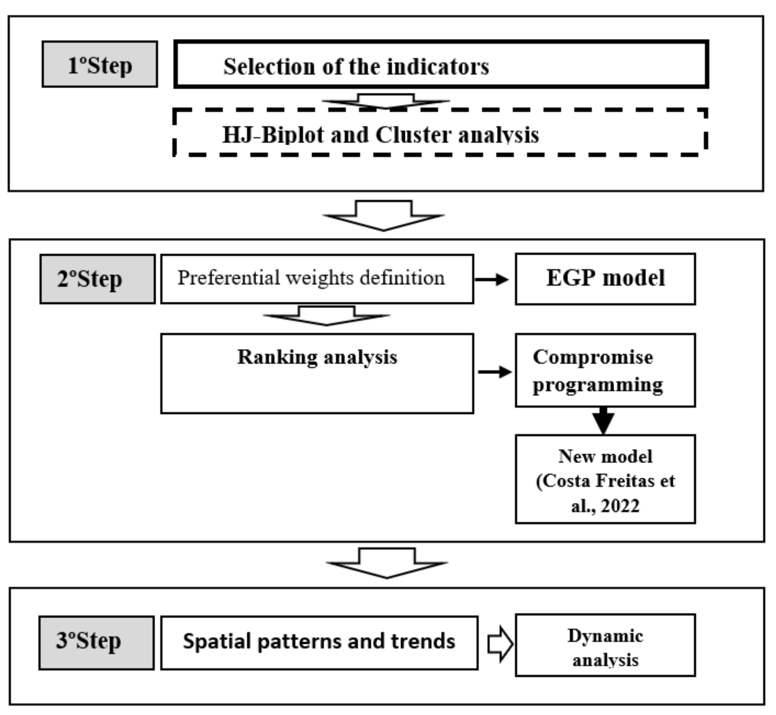
Figure 1. The methodological approach.
Sustainability 14 12512 g001
Figure 2. The study area.
Sustainability 14 12512 g002
Figure 3. The bidimensional HJ−Biplot representation. (source: model results).
Sustainability 14 12512 g003
Figure 4. The spatial distribution of the groups of municipalities. (source: model results).
Sustainability 14 12512 g004
Figure 5. The spatial distribution of the sustainability rankings in 2009. (source: model results).
Sustainability 14 12512 g005
Figure 6. The spatial distribution of the sustainability rankings in 2019. (source: model results).
Sustainability 14 12512 g006
Figure 7. Spatial dynamics of the sustainability rankings in 2009–2019. (source: model results).
Sustainability 14 12512 g007
Table 1. The selected agricultural sustainability indicators.
DimensionCodificationGeneral IndicatorDetailed DescriptionType
EconomicVPPEXPTotal Standard Output per farmTotal Standard output per farm (in Euros)More is better
VPP/SAU.Standard Output per hectareTotal Standard output value per hectare of utilized agricultural areaMore is better
TABANDAgricultural area evolutionIndicator of agricultural growth/abandonment expressed by the growth of the utilized agricultural area UAAMore is better
PATNGRFarms with other revenue sources)Proportion of farms with other revenue sources than agricultureMore is better
SocialMNFAMCreation of agricultural employmentShare of permanent labour that is hiredMore is better
PR65Aging of farmersProportion of farms’ managers with an age equal or higher than 65 years oldLess is better
EDAGRFarmers’ education and trainingProportion of singular producers with the 3º cycle (9º grade) or moreMore is better
IGENEDIRGender inequalityIndex of gender inequability ‘managersLess is better
EnvironmentalICULTHPESAgricultural system intensityImportance of the horticultural crops to the whole agricultural utilized land areaLess is better
CNSAULivestock unit per utilized agricultural landLivestock unit per hectare of utilized agricultural landLess is better
AGRBIOFarms with organic farmingPercentage of farms with organic farmingMore is better
ESTRAgricultural land with manure fertilization.Percentage of agricultural land in which manure was used.More is better
Table 2. The relative contributions of the factor to the element.
ColumnAxis 1Axis 2
VPP/SAU143341
VPPEXP335198
TABAND2314
PATNGR10199
MNFAM55572
IGENEDIR711137
EDAGR4129
PR651213
ICULTHPES0395
CNSAU22317
AGRBIO89117
ESTR406300
(source: model results).
Table 3. Ranking of sustainability for the ten best placed municipalities in 2009. (source: model results).
Ranking10.90.70.50.30.20
1BarrancosBarrancosBarrancosBarrancosBarrancosBarrancosAlcochete
2BenaventeBenaventeBenaventeBenaventeBenaventeBenaventeCartaxo
3Vila do CondeVila do CondeVila do CondeVila do CondeAlcocheteAlcocheteAlpiarça
4Alter do ChãoAlter do ChãoAlter do ChãoAlter do ChãoVila do CondeAlter do ChãoNazaré
5AvisAvisAvisAlcocheteAlter do ChãoVila do CondeRio Maior
6ArraiolosArraiolosArraiolosAvisAvisAvisAlmada
7Ferreira do AlentejoFerreira do AlentejoAlcocheteArraiolosArraiolosArraiolosLousã
8AlcocheteAlcocheteFerreira do AlentejoFerreira do AlentejoFerreira do AlentejoFerreira do AlentejoCaldas da Rainha
9Montemor-o-NovoMontemor-o-NovoMontemor-o-NovoMontemor-o-NovoMontemor-o-NovoMontemor-o-NovoAmares
10AljustrelAljustrelAljustrelAljustrelAljustrelAljustrelSetúbal
Table 4. Ranking of sustainability for the ten best placed municipalities in 2019. (source: model results).
Ranking10.90.70.50.30.20
1AlcocheteAlcocheteAlcocheteAlcocheteAlcocheteAlcocheteCartaxo
2MonforteMonforteMonforteMonforteMonforteMonforteLagos
3Alcácer do SalAlcácer do SalAlcácer do SalAlcácer do SalAlcácer do SalAlcácer do SalCaldas da Rainha
4ArraiolosArraiolosArraiolosArraiolosArraiolosArraiolosAlcochete
5Alter do ChãoAlter do ChãoAlter do ChãoAlter do ChãoAlter do ChãoAlter do ChãoAljezur
6AvisAvisAvisAvisVila do CondeVila do CondeAlpiarça
7Vila do CondeVila do CondeVila do CondeVila do CondeAvisAvisArmamar
8Montemor-o-NovoMontemor-o-NovoMontemor-o-NovoMontemor-o-NovoMontemor-o-NovoMontemor-o-NovoAmares
9CascaisCascaisCascaisCascaisCascaisCascaisBombarral
10Ferreira do AlentejoFerreira do AlentejoFerreira do AlentejoFerreira do AlentejoFerreira do AlentejoFerreira do AlentejoSintra
Table 5. Distribution of the ranking positions among groups of municipalities.
λ = 1
Group1–50.50–100.100–150.150–200.200–308.
Group 165224
Group 241320818
Group 335221051
Group 437564
Group 523132981
λ = 0
Group1–50.50–100.100–150.150–200.200–308.
Group 193025
Group 21777525
Group 312781136
Group 454844
Group 5729262838
(source: model results).
Publisher’s Note: MDPI stays neutral with regard to jurisdictional claims in published maps and institutional affiliations.