Groundwater Drought Analysis under Data Scarcity: The Case of the Salento Aquifer (Italy)

Abstract

Salento is a regional coastal karst aquifer located in Southern Italy with a highly complex geological, geomorphological, and hydrogeological structure. High and unruly exploitation of groundwater from licensed and unlicensed wells for irrigation and drinking purposes affects groundwater, with consequent degradation of its qualitative and quantitative status. The increased frequency of meteorological droughts and rising temperatures may only worsen the already compromised situation. The absence of complete and enduring monitoring of groundwater levels prevents the application of some methodologies, which require long time series. The analysis of climate indexes to describe the groundwater level variation is a possible approach under data scarcity. However, this approach may not be obvious for complex aquifers (in terms of scale, intrinsic properties, and boundary conditions) where the response of the groundwater to precipitation is not necessarily linear. Thus, the proposed research deals with the assessment of the response of the Salento aquifer to precipitation variability based on correlations between the Standardized Precipitation Index (SPI) and Standardized Precipitation and Evapotranspiration Index (SPEI) and groundwater levels for nine monitoring wells from July 2007 to December 2011. The study aims at evaluating the ability of the above indicators to explain the behavior of groundwater on complex aquifers. Moreover, it has the general aim to verify their more general reliable application. Results of three different correlation factors outline direct and statistically significant correlations between the time series. They describe the Salento aquifer as a slow filter, with a notable inertial behavior in response to meteorological events. The SPI 18-months demonstrates to be a viable candidate to predict the groundwater response to precipitation variability for the Salento aquifer.

1. Introduction

A groundwater drought might be defined as a lack of groundwater recharge or a lack of groundwater expressed in terms of storage or groundwater heads in a certain area and over a particular period [1]. Under natural conditions, groundwater droughts are recurrent phenomena that are due to precipitation deficiency under natural conditions and excessive exploitations. Although all droughts originate from a lack of rainfall, groundwater droughts take longer to manifest than meteorological droughts [1], depending on the scale of flow systems.

Currently, climate change represents a global topic of relevant interest and attention by both the scientific community and political decision-makers. The role of the climate trend (temperature increase and precipitation variations in space and time) on groundwater level is a crucial aspect for water resources planning and management. This aspect is essential considering the importance of groundwater further emphasized during meteorological drought due to the depletion of surface water resources [2].

Groundwater response to climate change is poorly investigated and the relationship between climate variables and groundwater level is more complex than that with surface water [3]. To assess the possible consequences of climate change for the future accessibility of groundwater resources, it is essential to understand the relationships between climate changes and drought occurrence and severity. This aspect is particularly significant for arid and semi-arid regions, such as the Mediterranean [4].

Van Loon and Van Lanen [5] remarked on the untrivial difference between drought and water scarcity. The term drought is correct when water is genuinely scarce; instead, the term water scarcity is relative to a condition caused by water use. The latter will increase in the future, considering population growth and a higher standard of living.

Despite groundwater being of critical importance for freshwater supply in many regions worldwide, in some areas, little management attention is paid to groundwater compared with more easily accessible surface water supplies, including stream flows and storage reservoirs. “Free for All” groundwater policies allow for higher exploitation of the water resource than natural recharge rates, and in some areas, groundwater levels more closely reflect pumping regimes than natural cycles [6]. In this setting, assessing how the human response to drought impacts groundwater resources is crucial to managing the effects of future climate variability [7,8].

Groundwater drought analysis in terms of duration, severity, and frequency provides important information for water resources management and planning.

Technical literature proposes several indexes to analyse groundwater drought. Bhuiyan [9] proposed the Standardized Water-Level Index (SWI) to monitor anomalies in groundwater level (GWL) as a correspondent of aquifer stress. Bloomfield and Marchant [10] correlated the Standardized Groundwater Index (SGI) and the Standardized Precipitation Index (SPI) to characterize the severity of groundwater drought events. Li and Rodell [11] calculated the Groundwater Drought Index (GWI) on the basis of groundwater storage simulated by the Catchment Land Surface Model [12] and compared the results to those computed based on the observed data.

However, all these groundwater drought indicators require long time-series data of GWLs that are sometimes unavailable.

We cannot perform the analysis of the evolution of water scarcity without a long GWL time series. Data referring to a short time interval are not able to define if the analysed period is crucial in terms of groundwater drought or if it is simply a bottom peak of a normal GWL evolution.

On the other hand, climatic data and especially precipitation are more easily available and could be a way to estimate the response of an aquifer in conditions of scarcity of data. Precipitation can be regarded as a leading indicator of GWLs, e.g., [13,14,15] by applying time series analysis [16,17], multiple linear regression models [18], data learning techniques (ANNs), Fuzzy Linear regression analysis [19], and satellite data analysis [20,21,22]. These factors are relevant for quantifying and monitoring droughts, as the temporal scales over which precipitation deficits accumulate distinguish different drought types. These differences make it easier to quantify the delays between meteorological and groundwater droughts. In this context, the Standardized Precipitation Index (SPI) developed by McKee et al. [23] has been widely used to investigate the impact of meteorological droughts on water resources and hydrological systems [24,25,26,27,28,29]. Several studies explored the usefulness of the SPI for assessing the groundwater response to precipitation variability [10,30,31,32,33]. The precipitation–groundwater relationship is considered to be a linear dynamic system [34]. The results of time series statistical analysis might allow for verifying the precipitation–groundwater linear dynamic behavior.

This paper describes the correlation between two drought indexes, SPI and SPEI, and GWLs for three years for the Salento aquifer, a coastal karst aquifer in Southern Italy (Puglia region), comparing three different statistical methodologies.

As far as the authors are aware, no other examples in the technical literature report the ability of SPI to describe the behavior of groundwater on aquifers particularly complex. If we can easily schematize a homogeneous and isotropic aquifer of small size as a linear reservoir, we cannot do the same for the Salento aquifer because of its size. Being a karst aquifer of regional dimension has many consequences, such as the spatial variability of rainfall, geological, and geological-structural aspects and intensity of drawdowns that vary from area to area, and the complexity of recharge processes driven by anisotropy, only to mention a few features. These aspects, therefore, make the case of Salento challenging as a test bed for analysis methods. If the methods used in the proposed research are effective in this complex context, this may demonstrate the generality of their applicability.

2. Materials and Methods

2.1. Study Area

The study area is located in the south-eastern part of Puglia (Salento Peninsula, Southern Italy), covering 2760 km². Its borders approximately coincide with those of the Lecce province. The Peninsula is bordered with the Ionian Sea to the west and the Adriatic Sea to the east (Figure 1).

The Salento Peninsula is part of the Apulia carbonate platform, characterized by a well-bedded succession of Jurassic-Cretaceous carbonate rocks with a thickness ranging from about 3 to 5 km. The geological basement, outcropping in large areas, shows sequences of massive and fractured/ karstified layers and banks of limestone and dolomitic limestone of Cretaceous age. The covers comprise sand, silty, or sandy clay, and calcarenite of Miocene to Pleistocene age [35]. Horst and graben structures, separated by a combination of gentle folds, E-W dextral and sinistral strike-slip faults, and NW-SE sub-vertical normal faults, typify the basement. Poor ephemeral stream networks drain the karst surface: they are mostly dry and cause flash floods discharging significant flows when heavy and intense precipitation occurs. In particular, the network drains the outflow of exoreic basins along the coast and converges inland into several endorheic basins, covering over 40% of the total study area [36].

The carbonate basement represents the main coastal aquifer for Salento Peninsula. Precipitation is about 600–700 mm/year and concentrates in the autumn-winter period (October–March). Several drought events from moderate to mild were identified in Salento Peninsula by Alfio et al. [37] in the period 1949–2011; a particularly severe drought was detected in 2006–2008. Hydraulic heads are very low, from highest values around 3 m above mean sea level (AMSL) in the southeastern part of the aquifer to less than 1 m AMSL at the coasts; their distribution suggests that groundwater may move according to a regional flow system. The mean hydraulic gradient is in the order of a few tenths per thousand.

Available data from deep wells distributed in the Peninsula show that freshwater floats on saltwater of marine origin (lower hydraulic limit) with freshwater maximum thicknesses around 120 m at the wells with the highest water levels. During the geological history, under the combined effect of complex tectonics and glacio-eustatic oscillations [38], the heterogeneous carbonate formation underwent vadose, water table, and transition-zone karstification, which made evolving its secondary porosity. Such processes shaped the basement surface, forming karst plains, endorheic basins, dolines, sinkholes, and the basement subsurface, making evolving secondary porosity of main faults and associated fracture zones, and shaping sub-horizontal levels. The set of discontinuities and karst forms constitutes an interconnected network characterized by a high anisotropy of the hydraulic conductivity. Groundwater mainly circulates in phreatic conditions. However, main faults appear to control groundwater flow by exhibiting conduit, conduit–barrier, or barrier behavior from place to place, thus causing compartmentalization of the aquifer at the regional scale [39]. In these large compartments, the heterogeneity of the carbonate sequences, often coupled with the displacements of the basement, leads groundwater to circulate to places in confined conditions.

The recharge conditions of the Salento aquifer are very complex and diversified according to the geological, tectonic, and morphological aspects. The surface area affected by endorheic basins, dolines, and associated swallow holes is the most prone for focused recharge, which also occurs where post-Cretaceous covers of low primary permeability crop out. There, discontinuous hydrographic networks of an endorheic nature favor recharge to the karst aquifer through the discontinuities defined by neo-tectonics, and through swallow holes that, although present on the covers, reflect the karstification of the underlying basement. The major discontinuities, often also crossing the covers, intersect the endorheic area, and play a different hydrogeological role according to the permeability along the damage zones, sometimes causing the compartmentalization of the aquifer.

The hydrological balance of the Salento aquifer is difficult to determine because of large uncertainties in evaluating both groundwater abstractions and coastal discharge.

2.2. Methods

This section reports the methodologies adopted to describe the behavior of the Salento aquifer in terms of groundwater variability from July 2007 to December 2011, using available monthly data. The analysis is based on the hypothesis of a potential correlation between SPI or SPEI with GWL. The correlation between climatic indices and GWLs may seem obvious, and potentially it is so if we schematize aquifers as simple linear reservoirs where precipitation is the input and GWL is the output. However, there are aquifers where the input and output largely vary over time and space.

The case study is complex as it is a regional coastal karst aquifer. Because of its spatial scale, it shows temporal and spatial variability of precipitations, which make variable the groundwater recharge. Moreover, the system is disturbed by consistent drawdowns for drinking and irrigation use. If climate indices prove to be effective in this case study in describing GWL variations and the response system to dry and wet periods, it would be relevant to state with certainty that these indexes alone can help simulate the response of the aquifer.

This study uses different correlation methods accompanied by a comparison of the results. A first analysis by the Kolmogorov–Smirnov test allowed to verify the normal distribution of SPI, SPEI, and GWL [40,41]. Then, the best suitable approach for the case study relied on the esteem of Pearson’s, Kendall’s, and Spearman’s correlation coefficients. Pearson product-moment correlation, Spearman’s rank-order correlation, and Kendall’s tau correlation are the most used measures of monotone association, with the latter two usually suggested for non-normally distributed data. These three correlation coefficients can be depicted as the differently weighted mean values of the same concordance factors.

Chon [42] investigated the intrinsic ability of Pearson’s, Spearman’s, and Kendall’s correlation coefficients to affect the statistical power of tests for monotone association in continuous data. The superiority of Pearson’s over Spearman’s and Kendall’s correlations stems from the fact that Pearson correlation better reflects the degree of concordance and discordance of pairs of observations for some types of distributions. The disadvantage of the Pearson product-moment correlation seems to be mainly due to its known sensitivity to outliers. For large samples in which the presence of outliers may be greater, the above limits are particularly noticeable.

2.2.1. The Standardized Precipitation Index (SPI)

The Standardized Precipitation Index (SPI) is a precipitation-based index proposed by McKee et al. [23] as measure of the severity and duration of meteorological drought. SPI quantifies precipitation deficit or surplus normalized through long-term precipitation records [43]. Accumulation periods of monthly precipitation time series vary from 1 to 48 months; thus, interpretations of SPI depend on the used time scale [44].

McKee et al. [23] defined four drought categories for the SPI (

Table 1. Dry period categories according to the SPI proposed by McKee et al. [23].

SPI Values	Drought Category
0 to −1.00	Mild drought
−1.00 to −1.50	Moderate drought
−1.50 to −2.00	Severe drought
≤−2.00	Extreme drought

). The 1- to 6-months SPI indicates short-term conditions: it reflects seasonal variations of precipitation and soil moisture, defining agricultural drought. The 9- to 12-months SPI shows long-term conditions in precipitation patterns, highlighting hydrological and even groundwater drought. Finally, the 48-months accounts for socio-economic impacts [45]. The World Meteorological Organization [46] considers the SPI as the most suitable approach for quantifying the degree of wetness or dryness conditions thanks to its several strengths. It requires only precipitation as unique input data, and its comparison with other drought indicators is feasible. However, we can recognize several potential disadvantages e.g., (i) the requirement for a long (at least 30 years) and consistent time series [47], (ii) concerning regional analysis, the inability of the index to identify areas that may be more drought inclined than others, and misleadingly large positive or negative SPI values at short time scales to regions with low precipitation [48].

In this paper, SPI calculation, based on monthly precipitation data over an accumulation period from 6- to 48-months, allowed estimation of hydrological impacts and exploring the drought variation at inter-annual time scales [49].

2.2.2. The Standardized Precipitation-Evapotranspiration Index (SPEI)

Some of the limitations of the SPI suggested testing the effectiveness of the SPEI as well. The Standardized Precipitation-Evapotranspiration Index (SPEI) was proposed by Vicente-Serrano et al. [50] as a measure of wetness and dryness conditions combining precipitation and evapotranspiration data. It is based on the same mathematical structure of the SPI, using accumulated climatic water balance instead of precipitation. The SPEI input data is the difference between precipitation and potential evapotranspiration (PET). The PET is the amount of evaporation and transpiration that would occur if a sufficient water source were available.

SPEI (which includes the effect of evapotranspiration) should have a better capability in simulating the behavior of the aquifer and the variability of the GWL than SPI. This makes even more sense in areas such as the Mediterranean, where temperatures are somewhat high in many months of the year. The use of SPI could overestimate the recharge of the aquifer.

Considering the available data, even if with the known limits of accuracy [51], the Thornthwaite method [52] was adopted for the estimation of the monthly PET (mm):

$$\mathrm{PET}=16\mathrm{K}{\left(\frac{10\mathrm{T}}{\mathrm{I}}\right)}^{\mathrm{m}}$$

(1)

where T is the monthly-mean temperature (°C), I is a heat index calculated as the sum of 12 monthly index values of i, m is a coefficient depending on I, and K is a correction coefficient computed as a function of the latitude and month,

$$\mathrm{i}={\left(\frac{\mathrm{T}}{5}\right)}^{1.514}$$

(2)

$$\mathrm{m}=6.75\times {10}^{-7}{\mathrm{I}}^3-7.71\times {10}^{-5}{\mathrm{I}}^2+1.79\times {10}^{-2}\mathrm{I}+0.492$$

(3)

$$\mathrm{K}=\left(\frac{\mathrm{N}}{12}\right)\left(\frac{\mathrm{NDM}}{30}\right)$$

(4)

in which NDM is the number of days of the month and N is the maximum number of sun hours:

$$\mathrm{N}=\left(\frac{24}{\mathsf{\pi }}\right){\mathsf{\varpi }}_{\mathrm{s}}$$

(5)

${\mathsf{\varpi }}_{\mathrm{s}}$ is the hourly angle of sun rising depending on the latitude δ (radians) and the solar declination φ (radians):

$${\mathsf{\varpi }}_{\mathrm{s}}=\arccos \left(-\tan \mathsf{\phi }\tan \mathsf{\delta }\right)$$

(6)

$$\mathsf{\delta }=0.4093\mathrm{sen}\left(\frac{2\mathsf{\pi }\mathrm{J}}{365}-1.405\right)$$

(7)

where J is the average Julian day of the month.

For the determination of dry periods, we referred to the same categories proposed by McKee et al. [23] and reported in Table 1.

2.2.3. Pearson’s Product-Moment Correlation Coefficient

The Pearson’s correlation coefficient [53] is a parametric method for measuring the linear dependence between two series. It ranges between −1 (inverse relationship i.e., when one variable increases, the other decreases) and +1 (direct relationship i.e., both variables move in the same direction). A value of zero indicates the absence of correlation.

Correlation analysis was carried out between SPI and GWL and SPEI and GWL to determine whether the two indexes are positively correlated, namely where an increasing/reduction of SPI and SPEI corresponds to a growth/decrease of GWL, respectively.

2.2.4. Kendall’s Tau Correlation Coefficient

The Kendall’s correlation coefficient [54] is a nonparametric indicator for evaluating the strength and direction of association between two variables measured on at least an ordinal scale. It is the nonparametric alternative to the Pearson’s product-moment correlation and Spearman’s rank-order correlation coefficient (especially in the case of small sample size with many tied ranks). This coefficient requires examining two assumptions before its use: (i) the variables should be measured in an ordinal or continuous scale, and (ii) it is suitable that the two variables follow a monotonic relationship.

For the presence of ties, the Tau-b statistic is calculated [55]. It ranges from −1 (negative association) to +1 (positive association) with a value of zero indicating the absence of association. The Kendall’s Tau-b coefficient is defined as:

$${\mathsf{\tau }}_{\mathrm{B}}=\frac{{\mathrm{n}}_{\mathrm{c}}-{\mathrm{n}}_{\mathrm{d}}}{\sqrt{\left({\mathrm{n}}_0-{\mathrm{n}}_1\right)\left({\mathrm{n}}_0-{\mathrm{n}}_2\right)}}$$

(8)

$${\mathrm{n}}_0=\mathrm{n}\left(\mathrm{n}-1\right)/2$$

(9)

$${\mathrm{n}}_1={{\displaystyle \sum }}_{\mathrm{i}}{\mathrm{t}}_{\mathrm{i}}\left({\mathrm{t}}_{\mathrm{i}}-1\right)/2$$

(10)

$${\mathrm{n}}_2={{\displaystyle \sum }}_{\mathrm{i}}{\mathrm{u}}_{\mathrm{j}}\left({\mathrm{u}}_{\mathrm{j}}-1\right)/2$$

(11)

in which n_c and n_d are, respectively, the number of concordant and discordant pairs, t_i is the number of tied values in the ith group of ties for the first quantity, and u_j is the number of tied values in the jth group of ties for the second quantity.

2.2.5. Spearman’s Rank-Order Correlation Coefficient

Spearman’s rank-order correlation coefficient [56] is a nonparametric indicator of the statistical dependence between the rankings of two variables. It allows for defining if the relationship between the two variables can be represented by a monotonic function. The mathematical structure of Spearman’s correlation coefficient is defined as the Pearson’s correlation coefficient substituting the values of the two variables with their ranks [57]. Thus, Pearson’s correlation coefficient evaluates the linear relationships; while Spearman’s correlation coefficient assesses monotonic relationships (whether linear or not). Moreover, for Spearman’s correlation coefficient, the sign of the estimated indicator defines the direction of association between the independent and the dependent variables: a positive coefficient indicates that both the two variables increase; while a negative value indicates that the dependent variable increases when the independent one decreases. A Spearman’s coefficient of zero denotes that no tendency exists between the two variables. As for the above correlation indicators, its magnitude ranges from −1 to +1.

2.3. Dataset

The analysis of the effects of precipitation variability on groundwater resources for the Salento aquifer was based on the use of the SPI and SPEI evaluated from 6- to 48-monthly accumulation times.

Drought index methodologies recommend that the time series of the hydrological input variables are not less than 30 years. However, in the absence of long series, SPI can also be calculated on as little as 20 years’ worth of data [58].

The Civil Protection of the Puglia Government has provided monthly data on the rainfall of the Salento aquifer. The available series presented different lengths and occurrences of data gaps. In the preliminary phase, thirteen stations were therefore selected (Novoli, Lecce, Copertino, Nardò, Otranto, Galatina, Maglie, Minervino di Lecce, Gallipoli, Vignacastrisi, Taviano, Ruffano, and Presicce) from 1951 to 2020. Figure 1 shows the considered rain gauges, and

Table 2. Main features of the selected rain gauge stations. Height refers to the elevation of the meteorological stations.

Rain Gauge	Latitude 1	Longitude 1	Height [m AMSL]	Monitoring Period
Novoli	40.37	18.05	51	1951–2020
Lecce	40.35	18.17	51	1951–2020
Copertino	40.27	18.05	34	1951–2020
Nardò	40.17	18.03	54	1951–2020
Otranto	40.15	18.48	27	1951–2020
Galatina	40.13	18.16	73	1951–2020
Maglie	40.10	18.28	102	1951–2020
Minervino	40.08	18.42	103	1951–2020
Gallipoli	40.05	17.99	31	1951–2020
Vignacastrisi	40.00	18.40	99	1951–2020
Taviano	39.97	18.08	65	1951–2020
Ruffano	39.97	18.26	134	1951–2020
Presicce	39.88	18.27	105	1951–2020

¹ Coordinates in decimal degrees (WGS84).

summarizes their main features.

The Civil Protection of the Puglia Government supplied fragmented records for the average temperature. To fill this gap, we considered for the analysis of drought indexes the monthly mean temperature data set of NOAA (https://psl.noaa.gov/data/gridded/data.ghcncams.html, accessed on 10 July 2021) of one station located in Salento Peninsula. The Climate Prediction Center, National Centers for Environmental Prediction, recently developed a station observation-based global land that measures monthly mean surface air temperature at 0.5 × 0.5 latitude-longitude resolution from 1948 to the present [59]. Dataset consists of the combination of two large individual data sets of station observations derived from the Global Historical Climatology Network version 2 and the Climate Anomaly Monitoring System (GHCN + CAMS). The quality of the temperature data is not the same as the rainfall data; however, considering the average altitude and the distance from the coast of the study area, the quality of the SPEI is not affected.

SPI and SPEI from 6- to 48-months were preliminarily calculated for the selected rain gauge stations of Salento using the monthly precipitations and monthly average air temperatures from 1951 to 2020 to deal with a general climatic description of the study area and to obtain data for comparison in the time window considered for the GWL analyses. For the sake of brevity, Figure 2 and Figure 3 show SPI and SPEI only for the Lecce station, respectively. As well as for the other stations, they show weak differences between SPI and SPEI. Generally, the drought severity reflected by the SPI is more significant than that shown by the SPEI [60]. Both SPI and SPEI for Lecce show an extreme drought event from 2016 to 2020, while for the other rain gauge stations they show in the same period dry events from moderate to severe.

The Geographical Information System of the Puglia Region (http://www.sit.puglia.it/portal/portale_cis/Corpi%20Idrici%20Sotterranei/Dati%20del%20Monitoraggio, accessed on 10 July 2021) provided groundwater level data. Groundwater dataset belongs to the Progetto Tiziano, a groundwater monitoring project run by the regional government to assess the qualitative and quantitative status of the Salento groundwater from 2007 to 2011. The selected monitoring wells equipped with automatic surveys are in static condition and the groundwater comes from continuous data registered every hour. Figure 1 shows the locations of the monitoring wells.

Table 3. Main features of the selected monitoring wells. Elevation refers to the height of ground surface measured in meters (AMSL); Well-Head Thickness is the distance from the head of the well to the ground surface, Well depth represents the depth calculated from the head of the well, and Available monitoring period refers to GWLs considered time series.

Well	Latitude 1	Longitude 1	Elevation [m AMSL]	Well-Head Thickness [m]	Well Depth [m]	Available Monitoring Period
LE_19/II S	40.293	18.299	34.557	0.605	227.0	June 2007–December 2011
LE_12/IIIS	40.295	18.065	42.065	0.646	62.5	June 2007–December 2011
LE_NC4	40.245	17.978	48.195	0.976	170.0	June 2007–December 2011
LE_LS21LE	40.026	18.217	154.621	0.503	230.0	October 2007–December 2011
LE_PS24LE	39.968	18.306	106.059	0.575	250.0	June 2007–December 2011
LE_PS17LE	40.149	18.229	76.685	0.566	250.0	June 2007–December 2011
LE_4/II S	40.420	18.165	22.681	0.810	100.0	June 2007–December 2011
LE_1/LR	40.241	18.166	51.412	0.508	210.0	June 2007–December 2011
LE_2/BS	40.085	18.280	86.984	0.463	113.0	June 2007–December 2011

¹ Coordinates in decimal degrees (WGS84).

summarizes their technical characteristics. The stratigraphic information for the monitoring wells is scarce, especially regarding the phreatic or confined groundwater condition. A total of two wells are clearly in phreatic condition (LE_1/LR and LE_LS21LE), for two other wells there are no data (LE_12/IIIS and LE_NC4), while the remaining wells are in a locally confined condition at variable elevations below sea level.

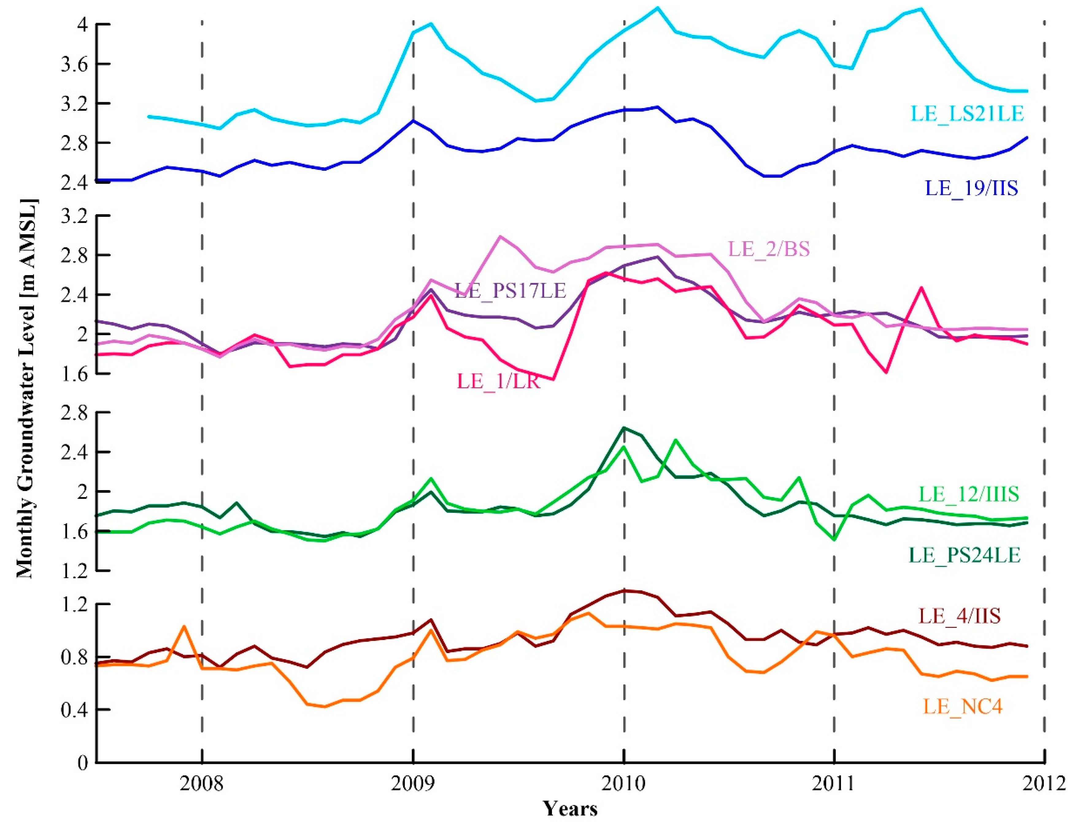
SPI and SPEI were compared with average monthly groundwater level of the selected nine monitoring wells from July 2007 to December 2011 (Figure 4). At first, each well was coupled with the nearest rainfall station; for this reason, we selected 5 rain gauge stations as candidate (i.e., Copertino, Galatina, Lecce, Maglie, and Ruffano). The validity of this approach was object to a subsequent validation by the spatial distribution of correlation coefficients between GWLs and SPI and SPEI time series.

3. Results

A preliminary statistical analysis of SPI, SPEI, and GWL datasets was made to determine if the time series were normally distributed. Results of Kolmogorov–Smirnov test showed that SPI and SPEI time series and all GWL records are normally distributed, with some exceptions (

Table 4. p-values of the Kolmogorov–Smirnov test for the selected reference periods of the SPI time series. Bold values highlight p-value below 0.05.

Rain Gauge	SPI-6	SPI-9	SPI-12	SPI-18	SPI-24	SPI-48
Copertino	0.63	0.51	0.23	0.023	0.43	0.05
Galatina	0.95	0.69	0.24	0.22	0.29	0.48
Lecce	0.52	0.14	0.005	0.041	0.32	0.24
Maglie	0.36	0.41	0.24	0.13	0.02	0.62
Ruffano	0.53	0.16	0.047	0.21	0.31	0.91

,

Table 5. p-values of the Kolmogorov–Smirnov test for the selected reference periods of SPEI time series. Bold values highlight p-value below 0.05.

Rain Gauge	SPEI-6	SPEI-9	SPEI-12	SPEI-18	SPEI-24	SPEI-48
Copertino	0.20	0.35	0.22	0.08	0.49	0.004
Galatina	0.81	0.65	0.14	0.1	0.39	0.45
Lecce	0.37	0.12	0.012	0.033	0.29	0.015
Maglie	0.75	0.57	0.08	0.1	0.037	0.19
Ruffano	0.77	0.29	0.033	0.08	0.67	0.54

and

Table 6. p-values of the Kolmogorov–Smirnov test for the GWL time series.

Well	GWL
LE_19/II S	0.56
LE_12/IIIS	0.75
LE_NC4	0.70
LE_LS21LE	0.56
LE_PS24LE	0.38
LE_PS17LE	0.74
LE_4/II S	0.74
LE_1/LR	0.47
LE_2/BS	0.22

).

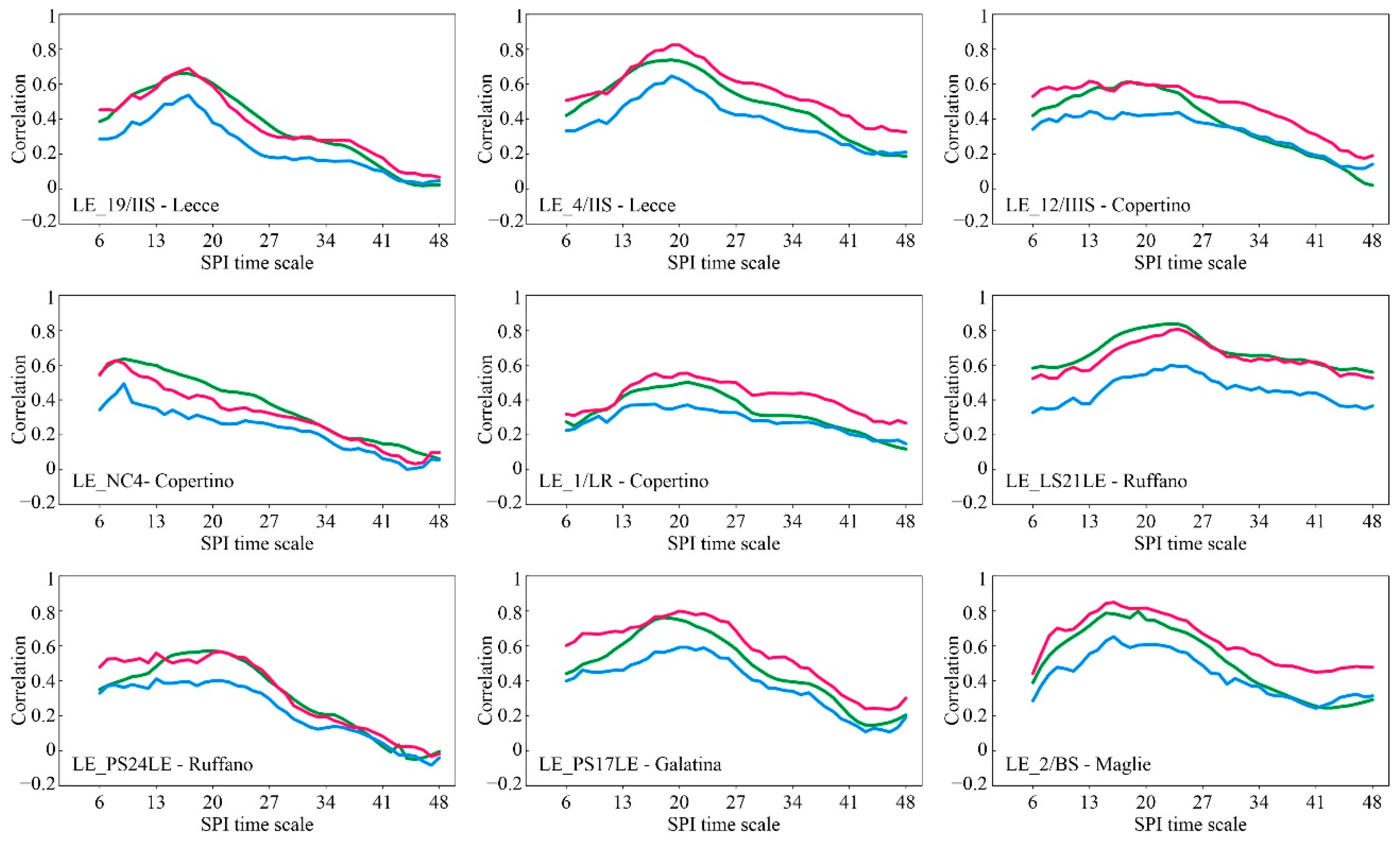
SPI and SPEI were compared with the monthly GWL from July 2007 to December 2011 according to three different methods. Results of the three different correlation coefficients were then compared. Figure 5 and Figure 6 show Pearson’s, Kendall’s, and Spearman’s correlation coefficients between SPI and SPEI from 6- to 48-months and GWLs, respectively. Results show that the curves of all correlation coefficients follow the same pattern for both SPI and SPEI. Each curve increases as it reaches the correlation peak and then slowly decreases to values, which are not statistically significant. Pearson’s and Spearman’s coefficients are similar, whereas those of Kendall’s are always lesser. The maximum correlation calculated at any time scale for the nine monitoring wells was greater than 0.60 for both Pearson’s and Spearman’s methods. Some wells (e.g., LE_LS21LE, LE_4/IIS, and LE_2/BS) reach the peak of correlation of about 0.85 for both SPI and SPEI. Moreover, different responses were detected with respect to the time scales of SPI and SPEI. All wells showed the highest correlation between 16 to 23 months with the exception of well LE_NC4 that presented the peak of correlation at 9 months. These different responses are recognized by all the three adopted methodologies. Furthermore, no significant differences were determined in the correlation between GWLs and SPEI compared to those obtained with SPI. In fact, the same range of maximum correlation and time responses can be identified for SPEI.

Because of the long response between GWLs and climatic indexes obtained in most cases, to visually compare GWLs with SPI time series, the representative time scale of 18 months was selected, except for LE_NC4 where the more representative time scale is 9-months. Thus, Figure 7 shows the selected monthly GWLs with the corresponding time scale from July 2007 to December 2011. It is noticeable that in all cases, the analysed period is characterized by a window of mild to moderate drought from the end of 2008, followed by a wet period, generally ending in early 2012. Groundwater level declines roughly correspond, in most of the cases, with drought events, whereas a rise in GWLs often exhibits fluctuations, which do not fit the SPI time series. The scatter plots between GWLs and the corresponding SPI for the more correlated time scale (18 months for all monitoring wells except 9-months for LE-NC4) of Figure 8 show quite low R-squared: the data are more dispersed in correspondence with the positive values of SPI.

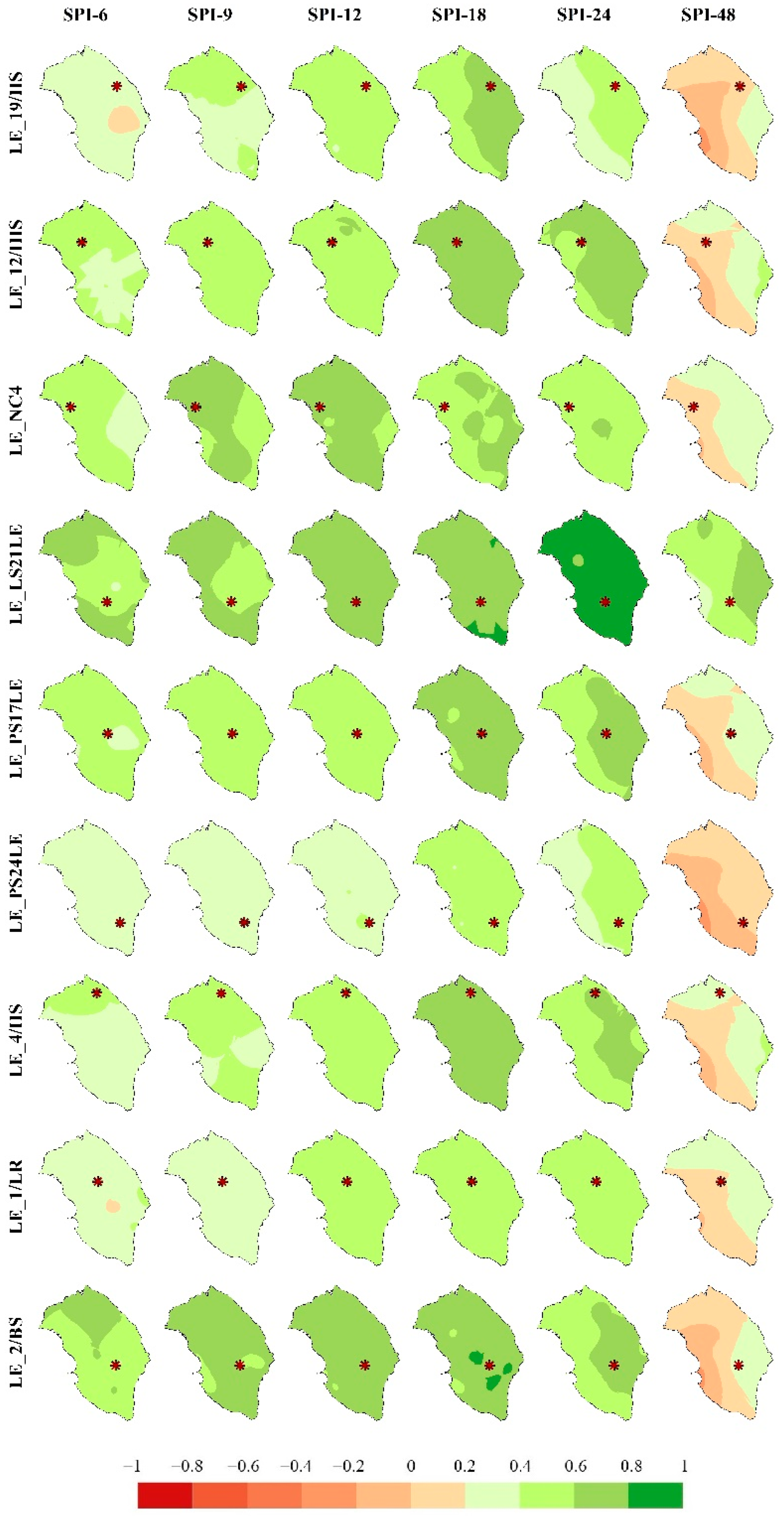
Figure 9 shows the spatial distribution of correlations between the GWL series for each well and the SPI series computed at 6, 9, 12, 24, and 48 months for all rain gauges using ordinary kriging. This analysis revealed that, in general, all GWLs display a positive correlation with most of the meteorological stations in Salento. Moreover, the recharge processes of the Salento aquifer depend on precipitation over broader areas so long as all the considered wells, except LE_NC4, showed a high or moderate correlation with the SPI 18-months, not within specific limited areas.

Frequently negative correlations with the SPI-48-month series occurred, indicating the strong independence of GWLs from too-long an accumulation time.

Only well LE_NC4 showed a high correlation with SPI 9- and 12-months, revealing a different behavior. The authors justified this considering this well is close to the Murgia regional aquifer (at the NW border of the Salento aquifer), which is characterized by high hydraulic heads. Maybe this well is affected by the proximity of this large aquifer, thus justifying its behavior compared to the other wells.

4. Discussion

The SPI and SPEI typically show a wide oscillation for a longer time scale, reflecting different types of droughts depending on the used time scale [61]. The longer the accumulation period for SPI and SPEI, the more prolonged in time and less frequent the drought events. In fact, dry events that occur at short intervals in SPI and SPEI-6 months tend to combine into a single prolonged event when moving to a higher accumulation period. SPI and SPEI time series in all rain gauge stations confirm the results of Alfio et al. [37] regarding the extreme drought which occurred at the end of the 1990s and moderate to severe droughts with few extreme droughts in the 2000s. The dry patterns shown by the SPI and SPEI are seriously alarming if we focus on the last few years of the processed series. These current droughts could distress groundwater levels, affecting both the quantitative and qualitative status of groundwater. The complex and heterogeneous structure of the Salento aquifer combined with the scarcity of the available time series of hydrological parameters makes the understanding of its hydrogeological behavior very challenging. Thus, a comparison of three different methodologies was made to determine the correlation between climatic indexes based on precipitation and temperature and GWLs. Pearson’s correlation defines the potential linear relationship between input and output, while Kendall’s and Spearman’s coefficients look for the possible existence of an association, which is not necessarily linear.

Results highlight a statistically significant positive correlation between SPI/SPEI and GWLs, with different time scales for each monitoring well and for the three methods, although with different rates. Pearson’s and Spearman’s correlation coefficients are better than those obtained by Kendall’s and similar to each other. This does not mean, however, that Kendall’s coefficients are less precise, but only that the relationship is evaluated from a different point of view. In fact, the three methods highlight similar correlation patterns from 6- to 48-monthly time scales. In general, the maximum correlation for each monitoring wells is detected for a long-time scale. Consequently, a potential linear relation between climatic indexes for a long accumulation scale and GWLs could be discussed for the Salento aquifer in the way that, despite the complexity, the aquifer linearly reacts to precipitation and temperature variability in the long term. This long-time response corroborates the results of another authors’ research not already published on the hydrodynamic behavior of the coastal karst aquifer of Salento, which behaves as a low-pass filter [62,63], with significant inertia in terms of transmissivity and storage capacity.

All the results confirmed the positive relationship between SPI and SPEI with GWLs. The results indicate the Pearson’s and Spearman correlation factors as the best methods to identify the relationship between precipitation and GWLs. In most cases, a long-time scale for SPI represents the more appropriate candidate in describing the effect of meteorological droughts on groundwater and its temporal variations.

Other notable aspects that come out from the results, besides the correlation between SPI and SPEI and GWLs, are the slow response of the system (on average 18 months for all wells except LE-NC4) and the different response of the system to dry and recharge periods. The data show that while, in most cases, the decreasing trends in GWL are consistent with the trends in SPI and SPEI about dry periods, the increasing trends do not fit in the same way.

This aspect is relevant if we consider that, concerning the management, what is most important is the prediction of groundwater droughts. The capability to predict the aquifer response to a period of meteorological drought allows for identifying priorities in terms of the water resource use.

For the same accumulation time, the values of Pearson’s correlation coefficients are slightly higher than those of SPEI. This aspect is not trivial considering that the Pearson’s method means a faster computation speed and a lower number of input parameters than the SPEI method. Moreover, the results confirm the existence of a linear correlation between precipitation and GWLs that is the underlying hypothesis for the Pearson’s method. Bloomfield and Marchant [18] early demonstrated this correlation by analyzing SGI rather than groundwater level records.

5. Conclusions

The research investigated the correlation between SPI and SPEI climatic indexes and GWLs of nine monitoring wells to look over the behavior of the Salento regional karst coastal aquifer during meteorological droughts. The aim was to explore the possibility of using indexes of meteorological drought to interpret groundwater level fluctuations in a complex aquifer with scarce data, where the inherent properties and boundary conditions can cause a greater level of complexity than expected groundwater level response during recovery and decline with significant rainfall and drought, respectively.

Pearson’s, Kendall’s and Spearman’s correlation methods were applied between SPI and SPEI and GWLs in a time window from July 2007 to December 2011. On the whole, results highlight a statistically significant direct correlation between hydrological and hydrogeological time series. Pearson’s correlation coefficient confirms a robust role in defining the relationship, which is of a linear type considering the assumptions of the method. As the higher correlations were detected for long-time scales, it can be assumed that the SPI-18 months are the best potential input parameters for this kind of analysis because the correlations of SPEI-18 were slightly lower. Therefore, the high correlation obtained with a high accumulation period explains the slow response of the aquifer to precipitation events, demonstrating the inertial behavior of the Salento aquifer. The reason for such inertial behavior could be linked to the recharge process. The recharge may occur through preferential pathways connecting the groundwater intercepted by each monitoring well with recharge areas even far away, which is rather normal in karst aquifers with high anisotropy of hydraulic conductivity. This is even more likely for those wells where groundwater is found locally confined.

The research results suggest that a similar approach may be applied to aquifers in complex environmental settings with scarce data. Unquestionably, similar methodologies are worthy of interest for those areas characterized by severe stress conditions due to long drought periods and under excessive groundwater exploitations.