Exploratory Spatial Data Analysis of Traffic Forecasting: A Case Study

Abstract

Transportation planning has historically relied on statistical models to analyze travel patterns across space and time. Recently, an urgency has developed in the United States to address outdated policies and approaches to infrastructure planning, design, and construction. Policymakers at the federal, state, and local levels are expressing greater interest in promoting and funding sustainable transportation infrastructure systems to reduce the damaging effects of pollutive emissions. Consequently, there is a growing trend of local agencies transitioning away from the traditional level-of-service measures to vehicle miles of travel (VMT) measures. However, planners are finding it difficult to leverage their investments in their regional travel demand network models and datasets in the transition. This paper evaluates the applicability of VMT forecasting and impact assessment using the current travel demand model for Dane County, Wisconsin. The main finding is that exploratory spatial data analysis of the derived data uncovered statistically significant spatial relationships and interactions that planners cannot sufficiently visualize using other methods. Planners can apply these techniques to identify places where focused VMT remediation measures for sustainable networks and environments can be most cost-effective.

1. Introduction

Many cities are experiencing congested roadways in areas that are largely built-out and lack room to expand. Hence, transportation agencies are seeking novel approaches to enhance mobility without expanding roadway capacities. Trucks in the European Union account for only 5% of vehicles, but they are responsible for 22% of the road transport carbon dioxide emissions, which analysts expect will grow [1]. Large freight users, such as distribution centers and intermodal transfer stations located outside metropolitan core areas, also contribute to increasing VMT levels. The growth of e-commerce, same-day deliveries, and the increasing focus on urban livability have increased the complexity and cost of urban logistics [2].

The continuous increase in truck miles of travel underscore the critical need for sustainable infrastructure management. Interviews with experts in city logistics suggest that demand management and public–private collaborations can be solutions [3]. A survey found that public sector initiatives to improve freight activity in metropolitan areas included infrastructure management, parking, and loading areas management, vehicle-related strategies, and traffic management [4]. Other initiatives included financial approaches, logistical management, and land use management [5].

Agencies such as the Wisconsin Department of Transportation (WisDOT) and many others issue guidelines for assessing land development impacts on adjacent state and federal highways. To assess mobility and land use impacts, most state agencies have adopted methodologies from the Highway Capacity Manual (HCM) to guide their facility designs. Those methodologies use highway level-of-service (LOS), which is a function of traffic volume and roadway capacities based on their existing geometry and condition [6]. For instance, guidance from the WisDOT’s Facilities Development Manual to transportation planners and engineers is to achieve the best practical LOS for intersections after considering local land use, economic, social, and environmental characteristics. Major state and federal facilities are expected to provide at least LOS D operating conditions at peak times for intersection movements [7].

As ubiquitous as the LOS evaluation metric of the HCM has become in contemporary highway planning and engineering, there is a growing movement to reset the nation’s transportation policies to assure sustainability and equitability for all users, and not only for vehicle owners. One predominant aspect of this movement has been to supplant LOS with a vehicle miles of travel (VMT) metric to shift the assessment of impacts from automobile mobility to more holistic quality-of-life measures. Agencies often refer to automobile trip reduction programs as transportation demand management (TDM), which seek to control growing levels of traffic congestion within cities. Evolving TDM programs encourage cost-effective alternatives to driving so that a sustainable transportation system becomes more viable as cities grow.

Comprehensive TDM programs have had limited success because they usually rely on both mandatory and voluntary compliance efforts to be successful. Public agencies have developed TDM programs based on their understanding of how people make their transportation decisions, but a predominate goal of TDM programs is to make better use of the existing infrastructure by replacing peak period single-occupant vehicle travel with transit, carpooling, walking, biking, and teleworking modes.

On a statewide level, California passed Senate Bill 743 in 2013 to mandate transportation system impact analyses, subject to the California Environmental Quality Act, transition from traditional LOS measures to VMT measures [8]. The purpose of this paper is to assess the effectiveness of several new VMT impact estimation methods as applied in San Jose, California by modifying a travel demand model developed for Dane County, Wisconsin. The main research questions are as follows:

• Can transportation agencies easily modify their existing LOS-based traffic demand models to reliably forecast VMT densities?
• How effective is exploratory spatial data analysis (ESDA) in revealing significant spatial relationships and visualizations that can inform cost-effective VMT remediation efforts?

Traditional statistical analysis identifies the expected, whereas ESDA helps to discover the unexpected. The literature review in the next section revealed that there are gaps in the use of ESDA to guide transportation planning based on VMT projections. Underlying methods of ESDA include spatial dependency tests to discover structures, trends, and underlying processes based on the data. A contribution of this research is to show how map clipping, data merging, base mapping, brushing, and linking tools provided additional insights by coupling data tables with maps to visualize year 2050 daily VMT within the Dane County, Wisconsin area.

The organization of the remainder of this paper is as follows: Section 2 conducts a literature review to provide background and discuss related works. Section 3 describes the ESDA methodologies utilized. Section 4 presents the data collected and the tools used to conduct the ESDA. Section 5 discusses the results. Section 6 concludes the study and summarizes new understandings gained.

2. Literature Review

Brundtland (1987) suggests that increases in human population have the power to radically alter our planetary system [9]. Consequently, our planet is undergoing major unintended changes in its atmosphere, soil, water, plants, and animals. Ramani (2018) found that key transportation agencies and actors in the United States have planning initiatives that target sustainability-related considerations such as livability, quality of life, and economic opportunity, but a cohesive and unified approach is lacking [10].

Recognizing the importance of environmental, health, and economic sustainability, the United States National Academy of Sciences commissioned a guidebook (NCHRP Report 708) to help state agencies identify and apply sustainability-related transportation performance measures [11]. The guidebook defined some fundamental principles of sustainability as meeting human needs for the present and future while preserving the environment, fostering community health, promoting economic prosperity, and ensuring equity among population groups. In a review of urban transportation planning, Sultana (2019) found that sustainability strategies tend to fall into the paradigms of changing mode and trip patterns to consume less resources and generate less waste, and making changes in the built environment to encourage more sustainable travel choices [12].

VMT measures how much people travel in vehicles. Low VMT areas mean people will not have to drive by car as much or as far to get what they need. Conversely, high-VMT areas mean people must drive further to get what they need and probably have fewer mobility options beside driving their cars. In transportation planning, moving from LOS to VMT performance measures requires a substantial commitment of time and resources. The literature generally recognized three transitional phases in the process: (1) preparation, (2) VMT modeling, and (3) implementation. Case studies have documented these phases of early VMT measure adaptors in the California cities of Los Angeles, Oakland, Pasadena, San Jose, and San Luis Obispo [13]. A survey found that California planners viewed VMT as a more appropriate measure for assessing environmental impacts than was LOS [14]. However, 44% of the survey respondents reported that they continue using LOS to measure development impact fees. Ferrell (2019) also noted that, while progress has been made in measuring the near-term direct VMT impacts from large-scale transportation projects since the passage of California SB 743, measuring the longer-term, indirect effects of development projects using VMT on surrounding areas remains a challenge [15].

In 2000, the U.S. Environmental Protection Agency (EPA) initiated a pilot program to evaluate a new Smart Growth INDEX (SGI) tool [16]. The SGI tool allowed users to benchmark existing environmental and community conditions and to evaluate the impacts of multiple development and transportation scenarios. The tool used a composite measure of household residents plus employees (HHEMP) to represent zonal density. The rationale was that both residents and employees generate distinct types of trips, even if they are the same persons.

A community’s desire to enact VMT reduction ordinances depends on how poor transportation service levels are affecting them and the degree to which the public supports government intervention [17]. VMT reduction initiatives have been either (1) efforts to reduce vehicle-related emissions [18] or (2) efforts to generate additional revenues needed to repair deteriorating pavements and bridges [19,20]. Transportation analysts widely agree that lowering VMT reduces greenhouse gasses, alleviates congestion, and reduces pollutants that are harmful to healthy communities, plants, and animal habitats [21,22]. VMT reduction tools applied at the local level can include road and parking pricing, mixed-use zoning, investments in alternative modes, and household travel planning programs. Each requires significant public investment, and their effectiveness is not verifiable until many years after implementation. However, there is some evidence that local actions can affect VMT sustainability by changing these policy-sensitive factors [23]. Case studies have also suggested that urban centers can support regional goals [24].

A few state governments such as California have passed legislation to reduce VMT. California targeted a 15% reduction in VMT within its communities by 2050 [25]. In accordance with new statewide policies, municipalities began developing new estimation methods and tools to comply with the statewide VMT reduction goals. Senate Bill 734 updated the way California agencies measured transportation impacts on land development projects, making certain they are built in a manner that gives Californians more options to drive less [8].

The city of San Jose was a frontrunner in developing and implementing processes to evaluate land development projects, which tied their VMT generation to population, jobs, and proximity to affordable housing [15]. City council action officially replaced LOS calculations with VMT as a measure of new development impacts. The city subsequently published new transportation impact guidelines for developers [26]. San Jose’s daily VMT per capita is 12 miles, and in accord with the new state law, their goal was to reduce the citywide average VMT by 15%. Community and transportation planners developed novel VMT forecasting tools based on empirical research, including a VMT calculator for development projects, normalized VMT reduction strategies by area type, and a spreadsheet-based impact workbook. Through their analyses, San Jose planners found that the large-scale transportation analysis zones (TAZs) of the regional model were too coarse to work with at their desired VMT target reduction scale. Hence, they also developed an algorithm that smoothed the VMT data of a model TAZ to the parcel level by weighting each parcel’s VMT by those of its surrounding parcels.

In summary, the literature reveals a hesitancy of agencies to transition from LOS to VMT as the key metric in facility planning because of their existing investments in LOS-based forecasting tools, rich datasets, and personnel trained on expensive software that are tuned to their needs. ESDA methods are still relatively new in transportation systems analysis, so agencies have not been applying them. This work seeks to fill those gaps by exploring how agencies can forecast VMT by using their existing datasets and tools and use ESDA to reveal statistically significant relations and patterns that can guide focused remediation efforts for environmental sustainability.

3. Methods

Case studies can challenge existing theories and practices. Unlike experiments, contextual conditions in case studies are not delineated or controlled, but instead become part of the investigation [27]. Following the case study approach, this research is descriptive rather than experimental, and the analysis is both quantitative and qualitative.

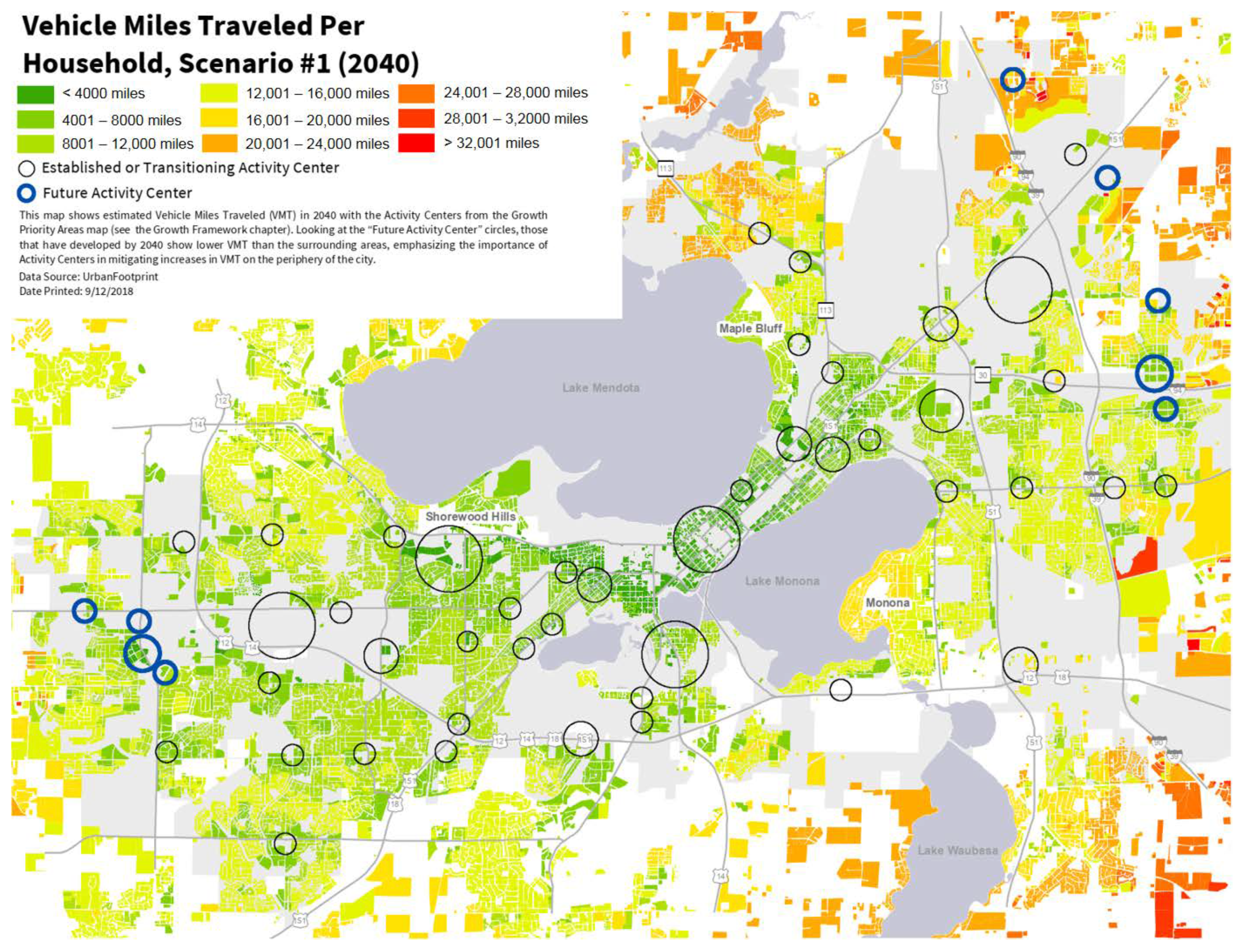
Madison is the largest city in Dane County and recently completed an update of its comprehensive plan. The city applied a growth scenario modeling tool called UrbanFootprint to estimate the impacts of land use and transportation decisions on future livability [28]. Figure 1 shows an example of Madison’s scenario #1 forecasted 2040 VMT-per-household using the UrbanFootprint program. Scenario #1 represented the baseline condition, with new city development having an edge growth focus. Based on the city’s comprehensive plan update, a greater reduction in VMT per capita and VMT per employee for the plan horizon year can be achieved by adding a new Bus Rapid Transit system, increasing express bus service, adding more traditional route bus service, and locating housing, jobs, and destinations nearer to each other and to regional transit hubs.

The colors on Figure 1 range from “cool” green to “hot” red to color-code the relative density of VMT per household for the locations shown. The city’s downtown area, which lies on a land isthmus between Lakes Mendota and Monona, has relatively high levels of transit service, dense employment centers, and significant mixed-use development. Consequently, the VMT-per-household in this area is relatively low. Conversely, the VMT-per-household increases toward the city’s outer limits where there are fewer options to reduce vehicular trips.

This research utilized the Dane County travel demand model to estimate horizon year VMT, since the authors were familiar with the unique datasets and the operational characteristics of the model. The VMT forecast used TAZ level data from the regional travel demand model. The workflow required two software platforms: CUBE Voyager^®, a transportation planning software by Bentley Systems, and GeoDA™, a publicly available tool used to conduct ESDA. CUBE provides a complete transportation GIS component, so it can deal directly with geodatabases and shapefiles [29]. GeoDA has tools to conduct a wide variety of spatial data analyses on lattice data that consists of points and polygons [30]. GeoDA links data across maps, tables, charts, and graphs to enable correspondence visualization. The linking feature enables several views of the same data within different analytical windows. Brushing is the program’s ability to immediately update all the views by dynamically selecting data with a movable shape within any analytical window. Figure 2 illustrates and summarizes the methodological workflow.

The Greater Madison Area Metropolitan Planning Organization (MPO) and WisDOT originally created the 2050 horizon year forecasts for population, households, employment used in the Dane County Regional Travel Demand model. Hence, the Dane County model has a base year and a forecast year of 2017 and 2050, respectively. The horizon year choice of 2050 reflected U.S. federal law (23 CFR § 450.312) that each planning organization regularly approve a transportation plan that forecasts demand for transportation facilities and services at least 20 years into the future [31]. The Madison MPO is currently producing an update titled “Connect Greater Madison: Regional Transportation Plan 2050 Update” [32]. The 2050 horizon year is also consistent with the VMT reduction goal timeframes for the City of San Jose [33].

The Dane County Travel Demand Model provided four data sets needed to estimate future year VMT:

• Geographical shapefile of the TAZ as polygons;
• Node-link highway network with attributes of travel speeds and capacities;
• Socioeconomic attributes of each TAZs; and
• Interzonal travel distance and trip tables.

The geodatabase shapefile used for the ESDA spatially joins the base and future year socio-economic variables to polygons, defined as TAZs. Dane County TAZs vary in size from small individual blocks to large census tracts. Smaller and larger TAZs are typically located within the isthmus and the rural areas, respectively. The travel demand model includes 1109 internal TAZs, as shown in Figure 3.

The workflow extracted the entire Dane County road network from the geodatabase and created “skims” of interzonal connections. Skims provide information about travel times, costs, and other travel impedances between zones based on the networks connecting them. A symmetrical matrix indexed by origin and destination zones stored the network skims. The same origin–destination matrix format stored trip tables. Each cell of the trip table matrix contained the trip volume of the corresponding origin-destination zone pair in the network. The diagonal of the trip matrix contained intrazonal trip volumes, which are the trips within a zone that do not enter the model’s highway network. The remaining steps were to:

• Multiply the trips in each cell by the corresponding distance to produce the VMT from each origin zone to each destination zone.
• Produce a corresponding zonal matrix of VMT.
• Sum the VMT from each origin zone to all destination zones to derive the VMT produced by each zone.
• Export the aggregated data to a comma-separated-value (CSV) file.
• Import the CSV into GeoDA for ESDA.

Figure 4 shows a screenshot of the CUBE Voyager code written to combine the individual time-period trip tables, add the distance skims to the matrix, combine trips from autos and trucks (excluding bus, walking, and bicycling trips), and multiply the vehicle trip table by the distance skim table for all origin–destination pairs. The “MW [9]” matrix is the sum of all daily truck and automobile trips across the eight time periods (three AM, three PM, one mid-day, and one nighttime), and the “MW [10]” matrix is the average distance for four trip types. The types of trips considered were home-based work (HBW) home-based shopping (HBSHOP), home-based office (HBO), and non-home-based (NHB) trips. The “MW [11]” matrix is the product of the daily trip volume and the average trip length, which is essentially the VMT.

The workflow normalized the VMT with zonal population, households, and employment data for comparison with other Wisconsin VMT databases and with the results from other locations such as San Jose. This analysis also adopted the composite measure (HHEMP) used in the EDA’s SGI tool as a measure of VMT density. This analysis used several ESDA methods for data visualization, including correlograms, heat-maps with natural breaks, scatter plots with regression, percentile maps, conditional maps, and k-means clustering.

Spatial correlograms graphically displayed covariances and correlations for pairs of observations as a function of the distance between them. Heat maps with natural breaks helped to visualize groups of maximum homogeneity or internal similarity. Scatter plots helped to assess the linear relationship between two variables. Percentile maps classified VMT data into a limited number of fixed ranges that highlighted the outliers. Conditional maps showed the spatial distributions of variables by isolating observations that fall into categories of the conditional variables. K-means clustering maps partitioned the VMT data into k groups, with k determined beforehand.

4. Results

Table 1. 2019 and 2050 VMT Comparisons.

2019 Base (WisDOT and US Census)			2050 Base (Dane Co. Model)
Measure	Dane County	VMT/Measure	Measure	Dane County	VMT/Measure
VMT	14,391,678	-	VMT	15,937,954	-
Population	546,695	26.32	Population	637,653	24.99
Households	222,929	64.56	Households	293,187	54.36
Employees	295,354	48.73	Employees	397,208	40.12

compares the Dane County demographic estimates and daily VMT for the most recent year available (2019) to those forecasted for the horizon year 2050. For comparability, the VMT per unit measure used the population, household, and employment data from the U.S. Census Bureau. The model forecasted that the Dane County daily VMT will increase by 1,546,276 miles by 2050 (10.74%), which is equivalent to an average annual growth rate of approximately 0.35 percent. However, the forecasted VMT per capita is projected to decrease by 5.05% over the same period, from 26.32 to 24.99.

The maximum number of zone pairs in the Dane County data is (1109² − 1109)/2 = 614,386. The bottom portion of Figure 5 shows the distribution of the number of zone pairs that fall within each spatial lag bin. The top of Figure 5 is a correlogram that shows the corresponding correlation coefficient for the VMT of those zone pairs. The intersection between the correlogram and the dashed zero axis determines the range of spatial autocorrelation, which ends around the midpoint of the fifth distance bin of 12,000 to 15,000 feet or approximately 2.5 miles. The number of zone pairs also peak at those lag distances. This result indicates that VMT trends are correlated within the urban core.

Heat maps highlight how the values of an attribute distribute spatially by showing darker and lighter colors as higher and lower values, respectively. Figure 6 color codes the model’s horizon year VMT-per-capita for Dane County TAZs using 10 natural breaks. Sixty-one of the 1109 zones (black colored) have undefined values because they are homogenous areas consisting of mostly public parks, conservancy lands, or commercial development without housing units. The heat map is consistent with those of the city’s UrbanFootprint analysis that showed VMT-per-capita is generally lowest in central Madison and increases radially outward.

Figure 7 shows a heat map of VMT by the EPA composite measure of households plus employment (HHEMP). The change in VMT density from the central city is more pronounced than for the VMT-per-capita measure.

Scatter plots can produce a visualization of the relationship between two attributes. Figure 8 plots the VMT against the composite EPA index HHEMP, both forecasted for 2050. The interpretation of the coefficient of variation (R-squared) is the percentage of HHEMP variance that explains the VMT variance. The p-value for the regression line is zero, which is less than the 0.05 significance level. Therefore, there is adequate statistical evidence to reject the null hypothesis that there is no correlation between VMT and HHEMP. In other words, that the HHEMP in 2050 (50HHEMP) is a statistically significant predictor of VMT.

The red circle in Figure 8 indicates major activity center outliers, which the linked map identifies as the East Towne Mall, West Towne Mall, Epic Medical Records Corporation, University of Wisconsin Hospitals, and the American Center (including American Family Insurance Headquarters and UW Health Clinics).

The map in Figure 9 plots the 2018 VMT-per-capita for San Jose [26]. Green areas on the map indicate parts of the city where the VMT metric meets the target threshold of 15% below the current citywide average. The yellow areas depict locations within the current city average. The orange areas are locations where the city would consider measures to reduce VMT to achieve the target density. The outer red areas are locations where the city expects that significant VMT reductions are not achievable.

Figure 10 provides a comparable map for Dane County. The 2050 average VMT per capita is 25 miles. The Dane County analysis zones are much larger than those of San Jose because the latter approximated smaller zones by estimating VMT at the land parcel scale by weighted regression with neighboring zones. The Dane County data in Figure 10 indicates that 663 zones (63.3%) are at or below the county average, and 385 zones (36.7%) are above the desired 2050 VMT per capita average.

Table 2. Summary of San Jose and Dane County VMT Target Reductions.

	San Jose Average (2018)	San Jose Target Threshold (−15%)	Dane Co. Average (2050)	Dane Co. Target Threshold (−15%)
VMT per Capita	11.91	10.12	24.99	21.24
VMT per Employee	14.37	12.21	40.13	34.10

shows the 2018 average VMT per capita for San Jose and the target value for VMT reductions. The table also shows similar data for Dane County, as derived from the regional transportation model for the year 2050. Figure 10 used the San Jose percentile thresholds but relative to the mean value forecasted for Dane County average. Therefore, values below 20.4 would be more than 15 percent below the target, and values within the range of 20.4 to 24.0 would be within 15 percent of the target. The county-wide average was within the 24.0 to 26.0 band. The VMT per capita range of 26.6 to 29.9 was 15 percent above the target, and the values above 29.9 was 15 percent above the County average.

Table 3. Dane County VMT per Capita Custom Map Breaks.

Zone Color	VMT Per Capita Threshold	No. of Zones (with Population)	Percent of Zones (with Population)	Comment
Light green	<20.4	422	40.3%	Predominately dense urban development with good access to high levels of public transportation.
Dark green	20.4–24.0	171	16.3%	Predominately on the urban fringe of the Madison area, generally outside the Beltline Highway and Interstate Highway 39/90/94.
Yellow	24.0–26.0	70	6.7%	Predominately suburban communities surrounding Madison.
Orange	26.0–29.9	135	12.9%	Predominately peripheral areas rural in nature typically aligned with major transportation routes.
Pink	>29.9	250	23.8%

provides further description the color coding used in Figure 10, the respective VMT ranges, and the VMT threshold criteria for Dane County.

Figure 11 shows a conditional plot of the horizon year VMT per capita for Dane County by quantiles of VMT and population. The color code is by percentile, where blue zones indicate those that fall in the 50% or lower percentile and the orange zones fall in the 50% or higher percentile. The lowest quartile VMT per capita are zones within the downtown Madison area.

The Moran’s I scatterplots and maps of Figure 12 depict Dane County zones with local indications of spatial association (LISA) where those relationships are statistically significant [34]. For each location, LISA indicates the degree of attribute similarity with neighboring zones. The criteria for neighboring zones are Rook, Queen, and distance. Rook criteria define neighboring zones as those that share a border, whereas Queen criteria adds corners to the criteria. Distance criteria are zones that fall within a predetermined radial distance threshold. There are five possible outcomes [35]:

• Locations with high VMT values and neighbors with high HHEMP values (high–high).
• Locations with low VMT values and neighbors with low HHEMP values (low–low).
• Locations with high VMT values and neighbors with low HHEMP values (high–low).
• Locations with low VMT values and neighbors with high HHEMP values (low–high).
• Locations with no significant local autocorrelation.

Table 4. Bivariate LISA (999 perm) with VMT and 50HHEMP and Moran’s I.

Cluster Mapped Zones	Rook Weighting	Queen’s Weighting	Distance Weighting
Not Significant	691	653	430
High–High	85	97	216
Low–Low	267	285	240
Low–High	52	52	201
High–Low	12	20	22
Moran’s I Stat.	0.196	0.193	0.126

summarizes the results of the three spatial weighting criteria applied. Generally, the significance of the Moran’s I results are lowest with rook weighting and highest with distance weighting at significance thresholds of p = 0.01 and p = 0.001. The high–high and low–low cluster associations also increase when moving from Rook to Queen criteria.

The global Moran’s I statistic indicates the presence of clustering in the overall pattern but cannot provide the location of the clusters. In Figure 12, the local Moran’s I cluster maps took the information from the Moran’s I significance maps and categorized spatial clusters that corresponded to the four quadrants of the Moran’s I scatterplot, but only for those areas below the p-value significance threshold. High–high and low–low clusters indicate zones with neighbors that have similarly qualified values relative to the means of the VMT and HHEMP attributes. High–low and low–high clusters indicate spatial outliers, which are zones with attribute values different from their neighbors.

Figure 12 indicates that there are several high–high clusters in Madison’s southcentral area, its upper northeast area, and in the urban core around the southwest area. It is notable that these zonal clusters occur along major transportation corridors in the city. In contrast, the distance weighted clustering results in more than twice the number of high-high clustered as compared with the Rook or Queen criteria, but they are much more dispersed around the city. There was a much higher number of low–high clusters when using the distance criteria for neighbors.

Figure 13 shows the results of k-means spatial clustering that separates the 1109 zones into eight groups based on the VMT/HHEMP density for 2050. The results show that the clusters grouped suburban communities together (colored in pink). The clustering method also grouped zones that are near the Madison Beltline and East Washington Avenue (colored in red).

5. Discussion

Cities experiencing increased congestion in built-out areas that lack room to expand presents crucial challenges to the transportation planners and engineers of today. Many segments of the population such as those with low income and the transportation disadvantaged who are seeking increased accessibility are demanding alternates to automobile travel to reach the critical goods and services needed for nearly all functions of modern life [12]. One promising answer has been to reduce the demand for new capacity by lowering VMT.

VMT and LOS are quite separate ways to measure how land development impacts traffic. VMT measures how much automobile and truck travel a development would create, whereas LOS measures the level of roadway congestion. LOS is proportional to the delay experienced by a motorist at an intersection relative to free-flowing traffic conditions. VMT measurements account for the positive effects of a quality transit service, walkable neighborhoods, and mixed-use development. Conversely, LOS improvements often lead to the widening of roadway corridors or intersection expansions, which encourages “induced traffic” due to the increased LOS [36].

The Dane County regional travel demand model produced VMT estimates for 2050 that were consistent with VMT estimates completed by the Wisconsin Department of Transportation. The Dane County VMT per capita was more than twice that of San Jose, thus reflecting a significant difference in the zonal network traffic and population characteristics of the two areas. However, the VMT density patterns of the two cities were similar. The low and average VMT per capita clustered near the city center and increased radially outward. A correlogram analysis revealed that the VMT trend for Dane County zones correlated up to a separation distance of 2.5 miles. Conditional mapping indicated that the lowest quartile VMT per capita were zones within the downtown Madison area. These results are consistent with the amount of mixed land use development and elevated levels of transit available in downtown Madison.

Scatterplot analysis of the data revealed a strong spatial correlation between the composite measure of households plus employment and VMT with outliers identified as the following five major activity centers: East Towne Mall, West Towne Mall, Epic Systems Corporation, University of Wisconsin Hospitals, and the American Center (American Family Insurance Headquarters, UW Health Clinics). There is limited space for roadway capacity expansion in or near major activity centers, which highlights why VMT mitigation measures would be more feasible and likely cost less than LOS improvement initiatives.

Mapping of significant spatial associations between VMT and HHEMP in the Madison area indicated that clusters formed in and around major activity regional centers and along principal arterial corridors. K-means cluster mapping grouped suburban communities and zones near the Madison Beltline and East Washington Avenue together. These patterns indicate that future VMT remediation strategies will need to focus on clusters that are forming away from the city centers while maintaining approaches that keep the VMT density in and near city centers within the desired limits. In particular, the analysis found that more than two-thirds of the Dane County zones were at or below the desired 2050 average VMT per capita.

A limitation of this approach is that, without significant modification, the TAZs of existing travel demand models are too geographically expansive for direct assessment of VMT reduction programs. However, it is possible to use smaller census blocks and create a weighted regression model that can estimate VMT based on population or population density, similar to what the City of San Jose did. This approach is justifiable based on the significant amount of VMT clustering into larger areas as observed in both the San Jose and Madison datasets.

6. Conclusions

Historically, United States infrastructure performance policies have prioritized an automobile-oriented system with little national interest shown in making fundamental changes in the way agencies evaluate traffic systems and make improvements. In recognition that transportation systems must continue to serve current generations without jeopardizing the welfare of future generations, governments have begun to seek an alternative to mobility management. Hence, there has been a gradual but consistent shift away from the level-of-service (LOS) metric of highway performance towards a vehicle miles of travel (VMT) metric. The motivation is to change the focus from supporting more highway traffic to planning for sustainable transportation systems and livable communities. However, the literature search revealed that such a change will be difficult and challenging for most transportation agencies because of existing investments in tools, datasets, and expertise. This work demonstrated that agencies can leverage their investments in the sociodemographic, traffic, and road network data currently used for travel demand modeling to effectively forecast VMT patterns. Subsequent exploratory spatial data analysis (ESDA) of the VMT and its various density derived measures can reveal patterns to inform agencies where to focus traffic remediation efforts and to maintain current practices that can help achieve sustainable transportation systems.

This work examined future VMT spatial trends in Dane County, Wisconsin using data from the existing travel demand model. Spatially analyzing VMT by TAZ for a transportation demand model horizon year is useful, but only practical when compared to baseline data of a similar nature. Additional work in this area should include reducing the analysis spatial scope from the entire Dane County area to only the greater Madison area to improve the spatial correlation. The smaller zones will enable the evaluation of various VMT reduction policies over time. Future work will smooth the TAZ data for the greater Madison area to land parcel sizes and compare those results with the city’s VMT analyzes using the UrbanFootprint tool.

References

- Filippova, R.; Buchoud, N. A Handbook on Sustainable Urban Mobility and Spatial Planning: Promoting Active Mobility; United Nations Economic Commission for Europe: New York, NY, USA, 2020; p. 234. [Google Scholar]
- Comi, A.; Savchenko, L. Last-mile delivering: Analysis of environment-friendly transport. Sustain. Cities Soc. 2021, 74, 103213. [Google Scholar] [CrossRef]
- Russo, F.; Comi, A. Investigating the effects of city logistics measures on the economy of the city. Sustainability 2020, 12, 1439. [Google Scholar] [CrossRef] [Green Version]
- Holguín-Veras, J.; Leal, J.A.; Sánchez-Diaz, I.; Browne, M.; Wojtowicz, J. State of the art and practice of urban freight management. Transp. Res. Part A Policy Pract. 2020, 137, 360–382. [Google Scholar] [CrossRef]
- Holguín-Veras, J.; Leal, J.A.; Sanchez-Diaz, I.; Browne, M.; Wojtowicz, J. State of the art and practice of urban freight management Part II: Financial approaches, logistics, and demand management. Transp. Res. Part A Policy Pract. 2020, 137, 383–410. [Google Scholar] [CrossRef]
- WisDOT. Traffic Impact Analysis Guidelines; Wisconsin Department of Transportation (WisDOT): Madison, WI, USA, 2021.
- WisDOT. Facilities Development Manual; Wisconsin Department of Transportation (WisDOT): Madison, WI, USA, 2020.
- Governor’s Office of Planning and Research. Technical Advisory on Evaluating Transportation Impacts in CEQA; Governor’s Office of Planning and Research: Sacramento, CA, USA, 2018. [Google Scholar]
- Brundtland, G.H. Our common future—Call for action. Environ. Conserv. 1987, 14, 291–294. [Google Scholar] [CrossRef]
- Ramani, T.; Zietsman, J.; Pryn, M.R. Towards sustainable transport planning in the United States. Eur. J. Transp. Infrastruct. Res. 2018, 18. [Google Scholar] [CrossRef]
- Zietsman, J.; Ramani, T.; Potter, J.; Reeder, V.; DeFlorio, J. NCHRP Report 708: A Guidebook for Sustainability Performance Measurement for Transportation Agencies; National Academies Press: Washington, DC, USA, 2011. [Google Scholar]
- Sultana, S.; Salon, D.; Kuby, M. Transportation sustainability in the urban context: A comprehensive review. Urban Geogr. 2019, 40, 279–308. [Google Scholar] [CrossRef]
- ChangeLab Solutions. How Measuring Vehicle Miles Traveled Can Promote Health Equity; ChangeLab Solutions: Oakland, CA, USA, 2019. [Google Scholar]
- Volker, J.M.B.; Kaylor, J.; Lee, A. A New Metric in Town: A Survey of Local Planners on California’s Switch from LOS to VMT. Transp. Find. 2019, 10817. [Google Scholar] [CrossRef]
- Ferrell, C.E. Measuring Incremental SB743 Progress: Accounting for Project Contributions Towards Reducing VMT Under California’s Senate Bill 743; Mineta Transportation Institute: San Jose, CA, USA, 2019. [Google Scholar]
- EPA. Smart Growth INDEX(r) 2.0: A Sketch Tool for Community Planning; Environmental Protection Agency (EPA): Washington, DC, USA, 2014.
- Sanford, E.; Ferguson, E. Overview of Trip Reduction Ordinances in the United States: The Vote is Still Out on their Effectiveness (Abridgment). Transp. Res. Rec. 1991, 1321, 135–137. [Google Scholar]
- Lee, S.; Lee, B. Comparing the impacts of local land use and urban spatial structure on household VMT and GHG emissions. J. Transp. Geogr. 2020, 84, 102694. [Google Scholar] [CrossRef]
- Hanley, P.F.; Kuhl, J.G. National Evaluation of Mileage-Based Charges for Drivers: Initial Results. Transp. Res. Rec. 2011, 2221, 10–18. [Google Scholar] [CrossRef]
- Litman, T. Are Vehicle Travel Reduction Targets Justified? Evaluating Mobility Management Policy Objectives Such As Targets To Reduce VMT And Increase Use Of Alternative Modes; Victoria Transport Policy Institute: Victoria, BC, Canada, 2021. [Google Scholar]
- Dulal, H.B.; Brodnig, G.; Onoriose, C.G. Climate change mitigation in the transport sector through urban planning: A review. Habitat Int. 2011, 35, 494–500. [Google Scholar] [CrossRef]
- Lee, A.E.; Handy, S.L. Leaving level-of-service behind: The implications of a shift to VMT impact metrics. Res. Transp. Bus. Manag. 2018, 29, 14–25. [Google Scholar] [CrossRef]
- Salon, D.; Boarnet, M.G.; Handy, S.; Spears, S.; Tal, G. How do local actions affect VMT? A critical review of the empirical evidence. Transp. Res. Part D—Transp. Environ. 2012, 17, 495–508. [Google Scholar] [CrossRef]
- Lewis, R.; Margerum, R.D. Do urban centers support regional goals? An assessment of regional planning in Denver. Land Use Policy 2020, 99, 104980. [Google Scholar] [CrossRef]
- CARB. California’s 2017 Climate Change Scoping Plan; California Air Resources Board (CARB): Sacramento, CA, USA, 2017.
- City of San Jose. Transportation Analysis Handbook; City of San Jose: San Jose, CA, USA, 2020. [Google Scholar]
- Ridder, H.G. The theory contribution of case study research designs. Bus. Res. 2017, 10, 281–305. [Google Scholar] [CrossRef] [Green Version]
- City of Madison Wisconsin. UrbanFootprint Analysis. Madison Comprehensive Plan Appendix C; City of Madison Wisconsin: Madison Wisconsin, WI, USA, 2017. [Google Scholar]
- Vorraa, T. Transport Modelling Supported By GIS—An Overview Of GIS Features Now Within Cube. WIT Trans. Built Environ. 2009, 107, 235–243. [Google Scholar]
- Anselin, L.; Syabri, I.; Kho, Y. GeoDa: An Introduction to Spatial Data Analysis. Geogr. Anal. 2006, 38, 5–22. [Google Scholar] [CrossRef]
- FHWA. Metropolitan Transportation Planning: Responsibilities, Cooperation, and Coordination; United States Federal Highway Administration (FHWA): El Paso, TX, USA, 1999. Available online: https://www.fhwa.dot.gov/legsregs/directives/fapg/Cfr450c.htm (accessed on 8 January 2022).
- GMMPO. Connect Greater Madison: Regional Transportation Plan 2050; Greater Madison Metropolitan Planning Organization (GMMPO): Madison, WI, USA, 2022. Available online: https://greatermadisonmpo.konveio.com/ (accessed on 8 January 2022).
- City of San Jose. Mobility: Vehicle Miles Traveled; City of San Jose: San Jose, CA, USA, 2018. Available online: https://www.sanjoseca.gov/your-government/departments-offices/environmental-services/climate-smart-san-jos/climate-smart-data-dashboard/mobility-vehicle-miles-traveled (accessed on 8 January 2022).
- Anselin, L. Local Indicators of Spatial Association—LISA. Geogr. Anal. 2010, 27, 93–115. [Google Scholar] [CrossRef]
- Oliveau, S.; Guilmoto, C. Spatial Correlation and Demography: Explorating India’s Demographic Patterns. 2005. Corpus ID: 2063057. Available online: https://www.semanticscholar.org/paper/Spatial-correlation-and-demography-%3A-explorating-Oliveau-Guilmoto/a469547ce66cfea19c69e17637d7ffacf7447fd0 (accessed on 8 January 2022).
- Volker, J.M.; Lee, A.E.; Handy, S. Induced Vehicle Travel in the Environmental Review Process. Transp. Res. Rec. 2020, 2674, 468–479. [Google Scholar] [CrossRef]