Analysis of Landscape Composition and Configuration Based on LULC Change Modeling

Abstract

Land cover changes threaten biodiversity by impacting the natural habitats and require careful and continuous assessment. The standard approach for assessing these changes is land cover modeling. The present study investigated the spatio-temporal changes in Land Use Land Cover (LULC) in the Gorgan River Basin (GRB) during the 1990–2020 period and predicted the changes by 2040. First, a change analysis employing satellite imagery from 1990 to 2020 was carried out. Then, the Multi-Layer Perceptron (MLP) technique was used to predict the transition potential. The accuracy rate, training RMS, and testing RMS of the artificial neural network, MLP, and the transition potential modeling were computed in order to evaluate the results. Utilizing projections for 2020, the prediction of land cover change was made. By contrasting the anticipated land cover map of 2020 with the actual land cover map of 2020, the accuracy of the model was evaluated. The LULC conditions in the future were predicted under two scenarios of the current change trend (scenario 1) and the ecological capability of the land (scenario 2) by 2040. Seven landscape metrics were considered, including Number of Patches, Patch Density, the Largest Patch Index, Edge Density, Landscape Shape Index, Patch Area, and Area-Weighted Mean Shape Index. Based on the Cramer coefficient, the most critical factors affecting LULC change were elevation, distance from forest, and experimental probability of change. For the 1990–2020 period, the LULC change was shown to be influenced by deforestation, reduced rangeland, and expansion of agricultural and residential areas. Based on scenario 1, the area of forest, agriculture, and rangeland would face −0.8, 0.5, and 0.1% changes in the total area, respectively. In scenario 2, the area of forest, agriculture, and rangeland would change by 0.1, −1.3, and 1.3% of the total area, respectively. Landscape metrics results indicated the destructive trend of the landscape during the 1990–2020 period. For improving the natural condition of the GRB, it is suggested to prioritize different areas in need of regeneration due to inappropriate LULC changes and take preventive and protective measures where changes in LULC were predicted in the future, taking into account land management conditions (scenario 2).

1. Introduction

Over the past decades, the effect of human activities on the planet has increased dramatically, resulting in a change in the landscape [1]. The change is associated with critical ecological consequences such as land use and vegetation changes, soil erosion, desertification, etc. The change usually has an obvious human source, but some morphological variables such as slope, direction, geologic formation, and elevation also contribute to the nature and extent of the change [2]. Land Use Land Cover (LULC) and its changes are essential variables that significantly impact the environment and its processes [3]. The change in the type of LULC not proportional to its capacity has increased the attrition process [4]. Understanding forest dynamics, sustainability conservation, and management evaluation methods depends on patterns, rates, and trend scenarios of land cover change [5]. Models of land cover change are tools that can be used to better understand the functioning of the land use system, analyze the causes and effects of landscape patterns, and support land cover management. In order to understand rates and geographical patterns of change and to estimate the effects of changes in land cover, these models’ applications harness a complex collection of economic-social and biophysical variables.

LULC heterogeneity quantification to study the relationship between spatial patterns and the occurrence of various natural processes is one of the critical approaches to landscape variations investigation [6,7,8]. The landscape metrics are considered proper tools for measuring the behavior of LULC as well as quantifying its effect on basin-scale processes and functions. These tools are also used for measuring and quantifying the spatial pattern of landscape changes [9]. The change detection process is another approach for investigating landscape changes and can be used for analyzing interactions between biophysical and human factors in socio-ecological systems [10]. These two approaches quantify the effects of land management on LULC changes and are helpful for modeling and describing management strategies in time and space at the basin scale [11]. The landscape metrics also investigate different dimensions of LULC changes such as composition, configuration, and connectivity at three levels: patch, class, and landscape [12].

Due to multiple landscape metrics, the most appropriate metrics should be selected according to the study aims as well as the result of the correlation between metrics. While the change detection processes investigate the landscape changes in each class of LULC over a period of time, in some cases, it is not easy to relate the change of landscape metrics to ecological process changes. Difficulties in investigating the LULC changes with a specific landscape metric force considering a set of driving factors [13,14,15]. One of the primary concerns of the researchers and land managers is the lack of insight regarding the changes and the effects of the landscape composition and configuration within the ecosystem on ecological processes [16,17]. Predicting the landscape pattern changes by considering ongoing change processes is vital to gaining insights into the status and behavior of LULC in the future and its effects on ecological processes. One way to deal with this is to develop a roadmap that can guide decision-makers and policymakers to efficient planning. For this, the impact of land use transition on the eco-environmental aspects needs to be considered [18].

Several studies have been conducted to investigate the behavior of the landscape and its effects on different processes. The authors of [19] investigated the landscape metrics in Haieh River Basin in China during the 1990–2000 period, demonstrating the need to quantify the pattern of the landscape. They concluded that the complex changes in the configuration and composition of the landscape during the study period are due to the importance of quantifying landscape patterns. The authors of [20] used landscape metrics to analyze urban land use patterns in different modes of urban development in Spain. According to their findings, landscape metrics can be used to monitor changes in urban development patterns and evaluate urban development policies. The study results of [21] on the landscape metrics in Uguraike, Japan, showed a reduction in the landscape diversity and dissection of water courses. The authors of [9] illustrated the temporal and spatial changes in agricultural land patterns using the landscape metrics, including scattering and proximity index in China. They emphasized the effectiveness of the method for investigating the development of agricultural lands at the basin scale. Modeling the effects of LULC change using the landscape metrics and hydrological features in the Calumpang Basin, Philippines, revealed that increasing the patch density and considering the largest patch index for forest and agriculture classes, respectively, resulted in reduced surface runoff and increased sediment production [22].

Land cover change models, in addition to landscape indices and change processes, can be helpful tools for comprehending a dynamic future landscape. To simulate how landscape aspects change over time and space and to investigate potential future possibilities, GIS models and RS data can be employed. The present study aimed to detect and analyze the changes in the landscape of the Gorgan River Basin (GRB) in northern Iran during the 1990–2020 period and predict the LULC map using the Land Change Modeler (LCM) based on two scenarios of continuation of the current change trend and based on the ecological capability of the land up to 2040. Despite the fact that extensive research on the interactions between LULC and landscape metrics has been carried out in several studies [23,24], to the authors’ knowledge, consideration of the temporal changes in land space processes, landscape metrics, and LULC have not been combined. To link landscape ecology with sustainable landscape development and planning, land space change processes were used. Therefore, this study comprehensively analyzes the landscape changes in a spatial framework considering the GRB’s landscape change processes and metrics.

2. Materials and Methods

2.1. Study Area

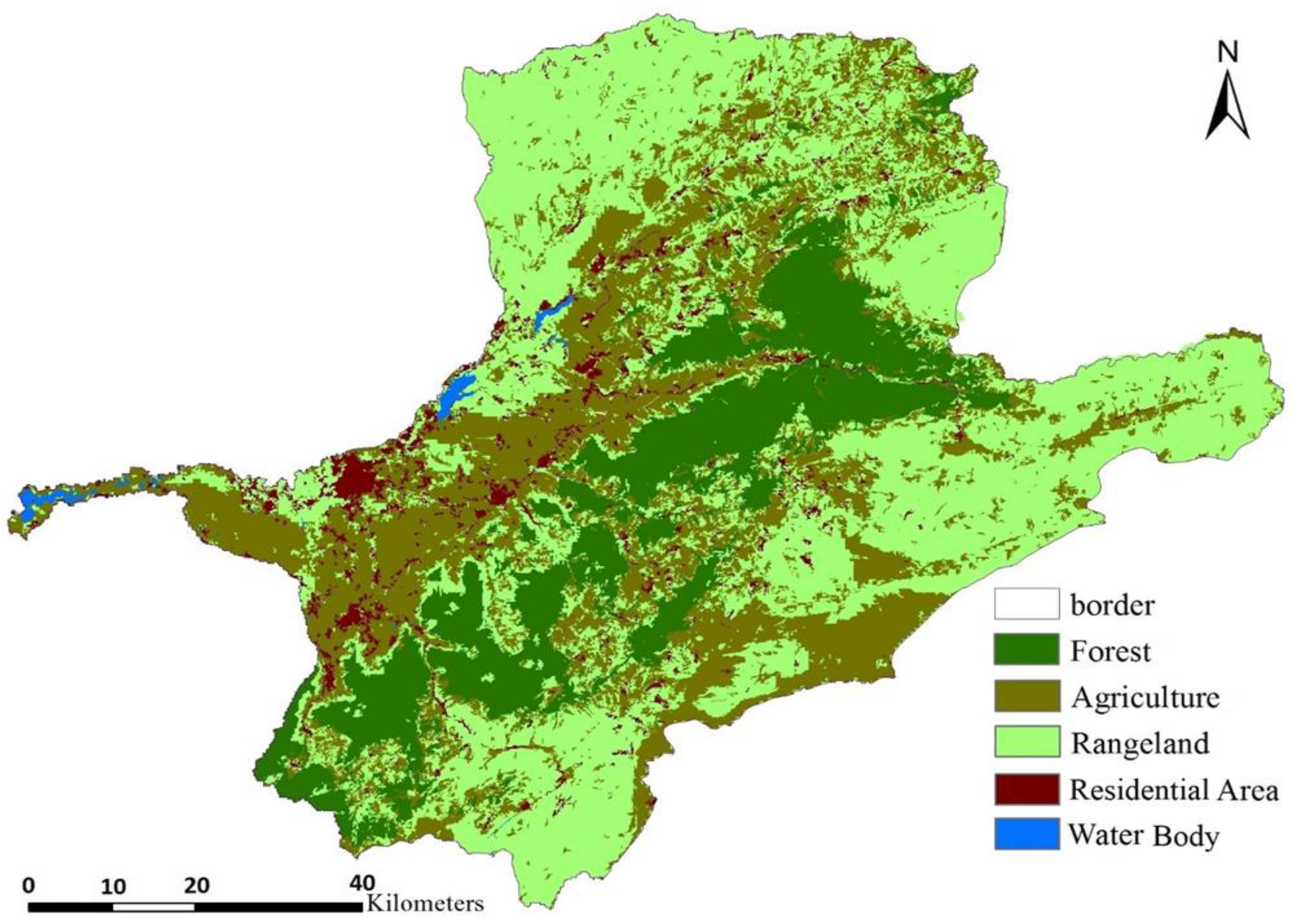
The GRB is located in northern Iran between 54° 42′ to 56° 28′ E longitude and 36° 43′ to 37° 49′ N latitude, with an area of 7138 km (Figure 1). The basin’s highest point is in the southwest Khoshyilagh region at an elevation of 2898 m above mean sea level (m amsl), and the lowest point is where the Voshmgir Dam is located, about 10 m amsl. The average elevation of the GRB is 890 m amsl with an average slope of 18% [25]. The longest river in the basin is known as the Gorgan River, which is 333 km long. The annual rainfall of the basin varies from 195.2 to 946.3 mm, with an average value of 620 mm. The minimum temperature is 11 °C and the maximum is 18.1 °C, measured in the Gorgan Dam climatology station.

2.2. Data Collection and Preparation

Four Landsat satellite images taken in 1990 and 2000 (TM Landsat-5), 2010 (ETM + Landsat-7), and 2020 (OLI Landsat-8) with 30 m resolution were acquired from the United States Geological Survey (USGS, https://earthexplorer.usgs.gov/ (June 1989, June 2000, June 2010, June 2019)). The images were projected onto the World Geodetic System (WGS) 1984, Universal Transverse Mercator (UTM), Zone 40 N coordinate system, and corrected geometrically with a first-order polynomial method using the nearest-neighbor algorithm [26]. The Root Mean Square Error (RMSE) of the images was less than one pixel. Contrast stretching and color composites were performed to enhance the interpretability of the images.

A 30 m Digital Elevation Model (DEM) was downloaded from the USGS site. The network road map (1:2000) was obtained from the Iranian Urban Development Organization. The main river map (1:2000) prepared by the Agricultural Organization of Iran was also acquired. The above-mentioned collected data were then used to create a Land Use Land Cover (LULC) map of the study area.

2.3. Land Use Land Cover (LULC) Classification

To properly identify and validate the phenomena that appeared on the images of TM, ETM+, and OLI sensors using true and false color combinations, field works were carried out, and educational samples for at least 50 sites in each class were collected randomly. For ground validation, the locations of the samples were spotted using a global positioning system (GPS) with high accuracy, and the land cover type at those locations was determined. Five classes were identified: forest, agricultural, rangeland, residential areas, and water body. The object-oriented classification algorithm, nearest neighbor [27], was used to classify satellite images using eCognition software and to generate LULC maps. The accuracy of the classified maps was evaluated by comparing the captured terrestrial reality points (30% of the actual data) with the classified map, kappa coefficient, and overall accuracy.

2.4. Land Use Land Cover (LULC) Calibration and Validation

We applied the Land Change Modeler (LCM) built-in module to model LULC change with a combination of different criteria. The input data required for Land Change Modeler (LCM) includes at least two land cover maps at different time periods. The amount of conversion, the spatial distribution of transitions, and gains and losses between land cover categories were calculated and analyzed for the periods 1990–2000, 2000–2010, and 1990–2010 by LCM for ecological sustainability [28]. According to the Kappa Index of Agreement (KIA) [29], the period of 1990–2010 was adopted in order to evaluate the model simulation. To transfer potential, the relationship between stimulus variables and user changes based on the Cramer coefficient was evaluated. Cramer’s $v$ is computed by taking the square root of the chi-squared statistic divided by the sample size and the length of the minimum dimension (Equation (1)). The LULC map of 2020 was predicted using LULC maps of 1990 and 2010 and was assessed based on a comparison with the 2020 terrestrial reality map. In the next step, the LULC map was predicted for future conditions (2040) using LULC maps of 1990 and 2010. The choice of 2040 was based on the need for approximately the same calibration, validation, and prediction periods [30], as well as the occurrence of LULC significant changes in the future. Therefore, the periods 1990–2010, 2010–2020, and 2020–2040 were selected as calibration, validation, and prediction of GRB’s LULC maps, respectively.

$$v=\sqrt{\frac{{\chi }^2}{N\left(K-1\right)}}$$

(1)

where χ² is derived from Pearson’s chi-squared test, N is the grand total of observation, and K is the number of rows or the number of columns, whichever is less.

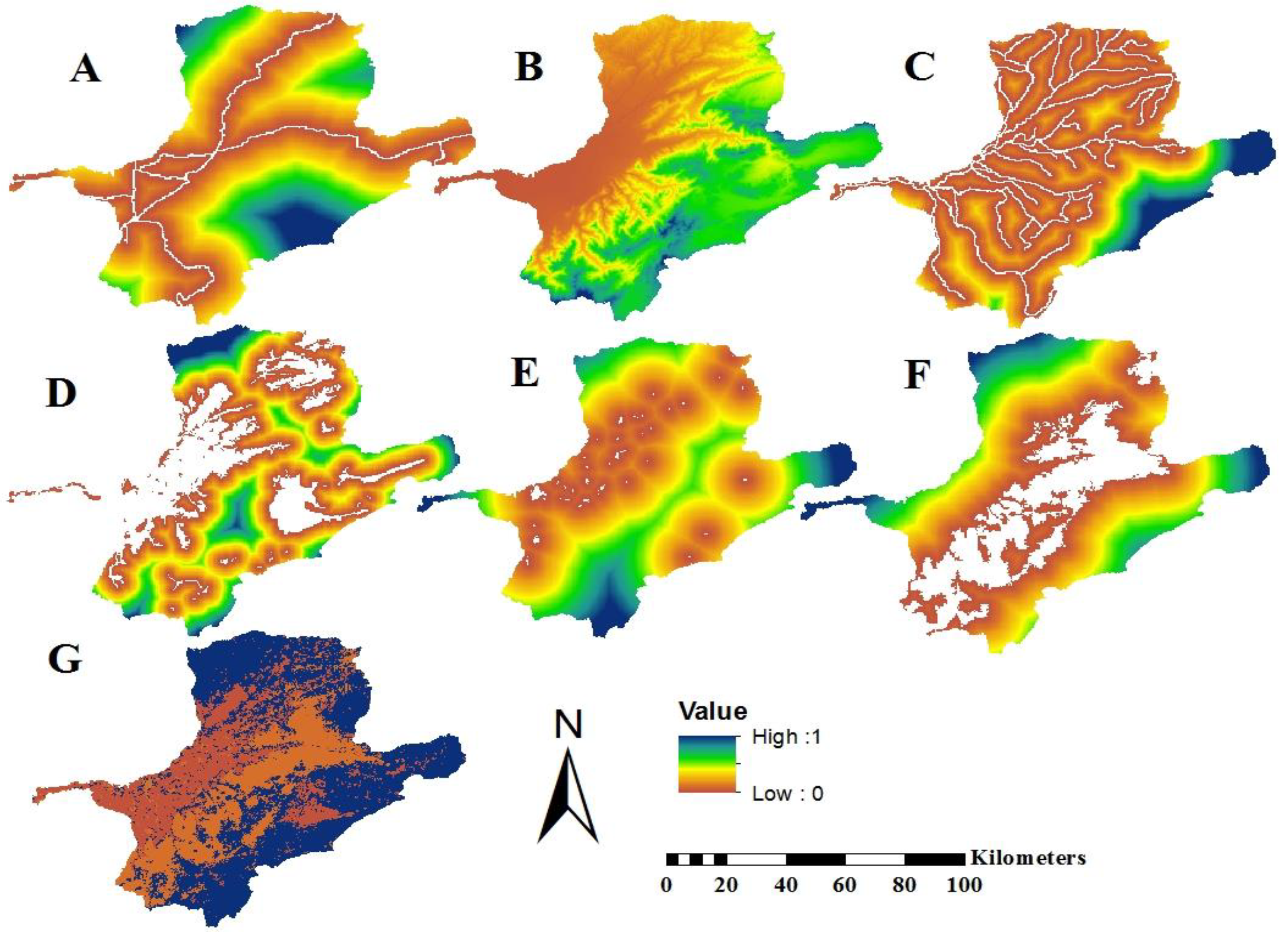
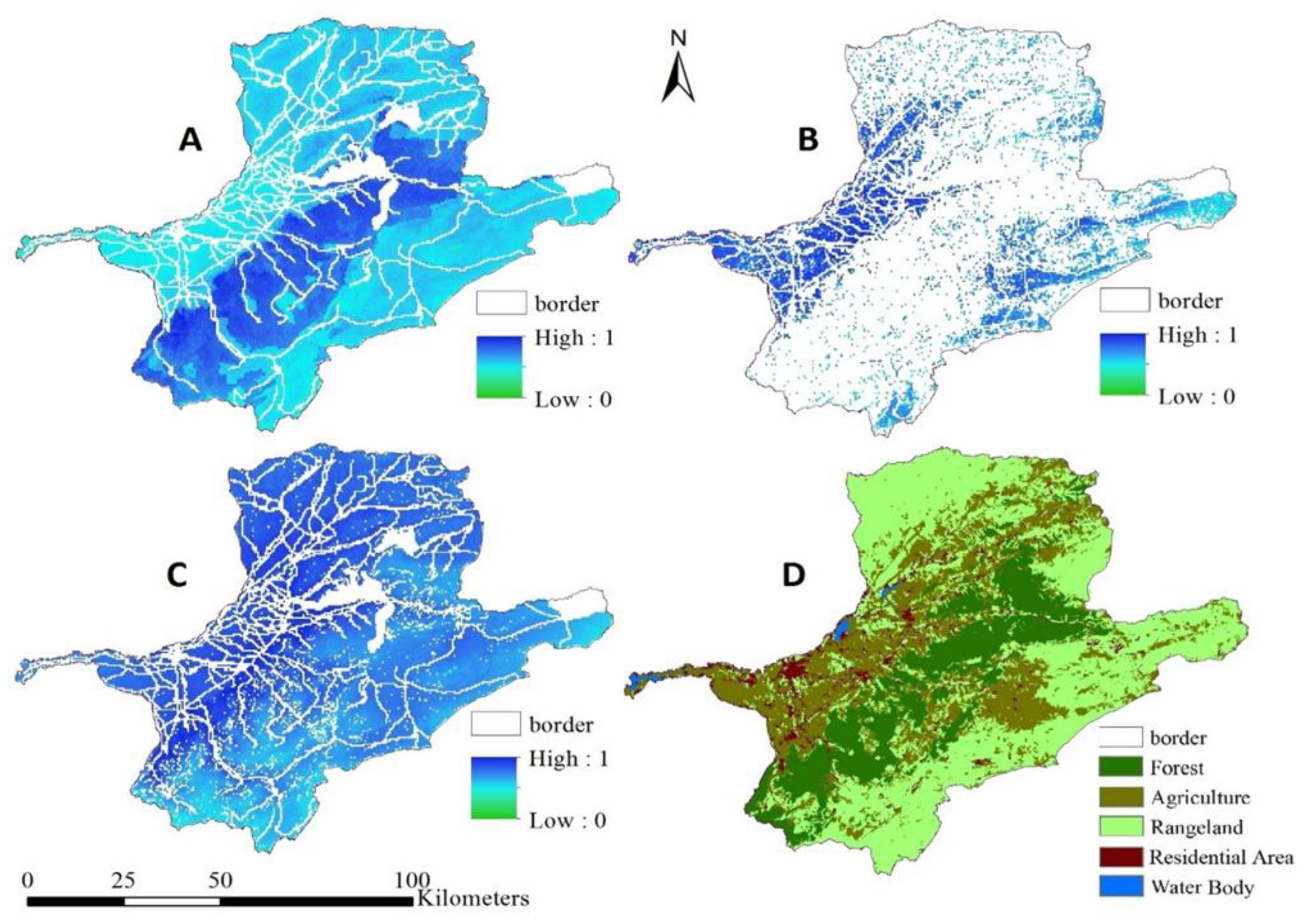
Digital Elevation Model (DEM), distance to forest, distance to a residential area, distance to agricultural lands, distance to the river, and distance to the road were considered explanatory variables in modeling transfer potential. The empirical likelihood was also generated in the modeling process, which is the expectance of changes in each land use class based on the effects of considered criteria (Figure 2).

2.5. Prediction of LULC Changes by 2040 Based on the Current Change Trend Scenario

In scenario 1, LULC changes during calibration and validation periods were analyzed by investigating the LULC change using the LCM. The LULC future condition map was predicted by selecting sub-models with the highest level of changes, including agricultural lands to rangeland, forest to agricultural lands, forest to range lands, rangeland, and agricultural lands to residential areas for modeling LCM transfer potential. The variables affecting LULC change were selected according to the literature review [31,32] as well as the availability of data. The Cramer correlation coefficient determines the relationship between explanatory variables (dynamic or static) and LULC classes based on Chi-square statistics so that values higher than 0.15 are acceptable [33].

Finally, the multilayer perceptron neural network (MLP) method was used, as one of the robust and common methods, for modeling the transfer potential [34,35]. In order to evaluate the accuracy of transfer potential modeling results, training error, test error, and accuracy indicators were used.

In the next step, the LULC changes based on the assumed future conditions were predicted by the Markov chain method [36]. The Markov model simulates the probability of future developments of the past land use types. According to the law of the Markov processes, the annual change rate of land use structure is rather stable. Equation (2) is the fundamental equation for predicting land use structure in the Markov process, in accordance with the concept of conditional probability.

$$P_{ij}^{\left(n\right)}={\displaystyle \sum }_{k=0}^{n-1}{P}_{ik}{P}_{kj}^{\left(n-1\right)}={\displaystyle \sum }_{k=0}^{n-1}{P}_{ik}^{\left(n-1\right)}{P}_{kj}$$

(2)

where n is the number of transfer steps, $P_{ij}^n$ is the probability of land type i change to land type j after n steps [37].

The predicted LULC maps were then evaluated by statistical and visual approaches using different kappa coefficients and figures of merit [38,39]. The value 0 and 100 figures of merit show inconsistency and consistency of the predicted map with terrestrial reality, respectively. The higher the value of the figure of merit, the higher the accuracy of the predicted map. The figure of merit is calculated using Equation (3).

FOM = H/(H + M + FL)

(3)

where hit (H) is the number of cells that have changed in terrestrial reality and have been correctly predicted by the model. Miss (M) is the number of cells that have changed in terrestrial reality but have remained constant in prediction. False alarm (FL) is the number of cells that have remained constant in terrestrial reality but have changed in model prediction.

2.6. Prediction of LULC Future Changes Based on the Land Ecological Capability

In this (scenario 2), future land use changes were made based on the ecological potential of the land using the weighted linear combination (WLC) method and the ecological models of Iran. In order to use the land resources for the development of land use change, a land utility map was prepared for the three major classes of forest, rangeland, and agriculture, subjected to major changes during the study period. The primary goal for obtaining the utility map of the area for the three major classes using the MCE method are as follows: (1) goal setting and identification of effective criteria; (2) standardization of criteria (constraint and factor); (3) weight of factors; and (4) integration using weighted linear combination (WLC) method. In the next step, 10% of the most capable areas were allocated to each class that subjects to change by 2040. The basis of this method is to select the patches that have the highest value to change for each class. In order to achieve this goal, several criteria were evaluated, using the multi-criteria evaluation (MCE) method developed [40].

In this scenario, the weighted linear combination (WLC) method, which is one of the most common techniques for multi-criteria evaluation and decision analysis, overlays standardized maps of factors taking into account the corresponding weights and Boolean layers of constraints. The final raster map is the utility map for the development of each land use that was integrated.

2.7. Preparation of Map of Limitations and Criteria for Standardization and Weighting

Identifying and developing criteria is the first stage of the multi-criteria evaluation process. The criteria include two categories of constraint and factor. The constraints are prepared in the form of Boolean layers, and factors are in the form of fuzzy layers, and according to the criteria they can be standardized in different ways. The fuzzy layers were created by the fuzzy membership algorithm. In this study, linear functions and, in some cases, user-defined functions were used.

The factors used to evaluate agriculture class potential include rangeland, geology, soil, erosion, climate, water resources, LULC, elevation, slope, direction, vegetation density, distance to villages, distance to roads, and distance to the city. These layers were fuzzy in different ways according to the type of layer. Further, to implement the multi-criteria evaluation method for each factor, a weight should be considered for each factor calculated based on the expert opinion and by the analytical hierarchical process.

2.8. Combining Criteria by Weighted Linear Combination (WLC) Method

The next step in the multi-criteria evaluation method is layer integration. In the present evaluation, the weighted linear combination method was used for layer integration. In this method, the criteria are standardized in a continuous numerical range and then combined based on weight averaging. First, the factors are summed based on the assigned weight. The resulting layer is then multiplied by the constraint layers to obtain a fuzzy layer that represents the utility of the whole area. The weighted linear combination method is calculated based on Equation (4).

$$S=\sum \left(Wi\ast Xi\right)\ast Cj$$

(4)

where S is LULC capability in each pixel. Wi is the weight of each criterion, Xi is the value of the fuzzy layer in each pixel (factor), and Cj is the constraint value in each pixel.

2.9. Extraction of Landscape Metrics

In order to investigate the dynamics of changes in the GRB landscape metrics, 7 metrics (

Table 1. Metrics specifications in each class and landscape level in the present study.

Metric Name	Acronym	Formula	Unit	Range	References
Number of Patch	NP	ni	unitless	NP ≥ 1	[41]
Patch Density	PD	$\frac{n_i}{A}$(10,000)(100)	number/100 ha	PD > 0	[22,41]
Largest Patch Index	LPI	$\frac{{}_{j=1}{}^n\mathrm{m}\mathrm{a}\mathrm{x}\left(a_{ij}\right)}{A}\left(100\right)$	%	100–0	[42]
Edge Density	ED	$ED=\raisebox{1ex}{${{\displaystyle \sum }}_{k=1}^{m\prime }{e}_{ik}$}\!\left/ \!\raisebox{-1ex}{$A$}\right.$	meters/ha	ED > 0	[41]
Landscape Shape Index	LSI	$\raisebox{1ex}{$0.25{{\displaystyle \sum }}_{k=1}^m{e}_{ik}$}\!\left/ \!\raisebox{-1ex}{$\sqrt{A}$}\right.$	unitless	LSI ≥ 1	[22]
Patch Area	PA	$PA=a_{ij}\ast \raisebox{1ex}{$1$}\!\left/ \!\raisebox{-1ex}{$\mathrm{10,000}$}\right.$	ha	PA > 0	[18]
Area Weighted Mean Shape Index	AWMSI	$\raisebox{1ex}{$0.25P_{ij}$}\!\left/ \!\raisebox{-1ex}{$\sqrt{a_{ij}}$}\right.$	unitless	AWMSI ≥ 1	[41]

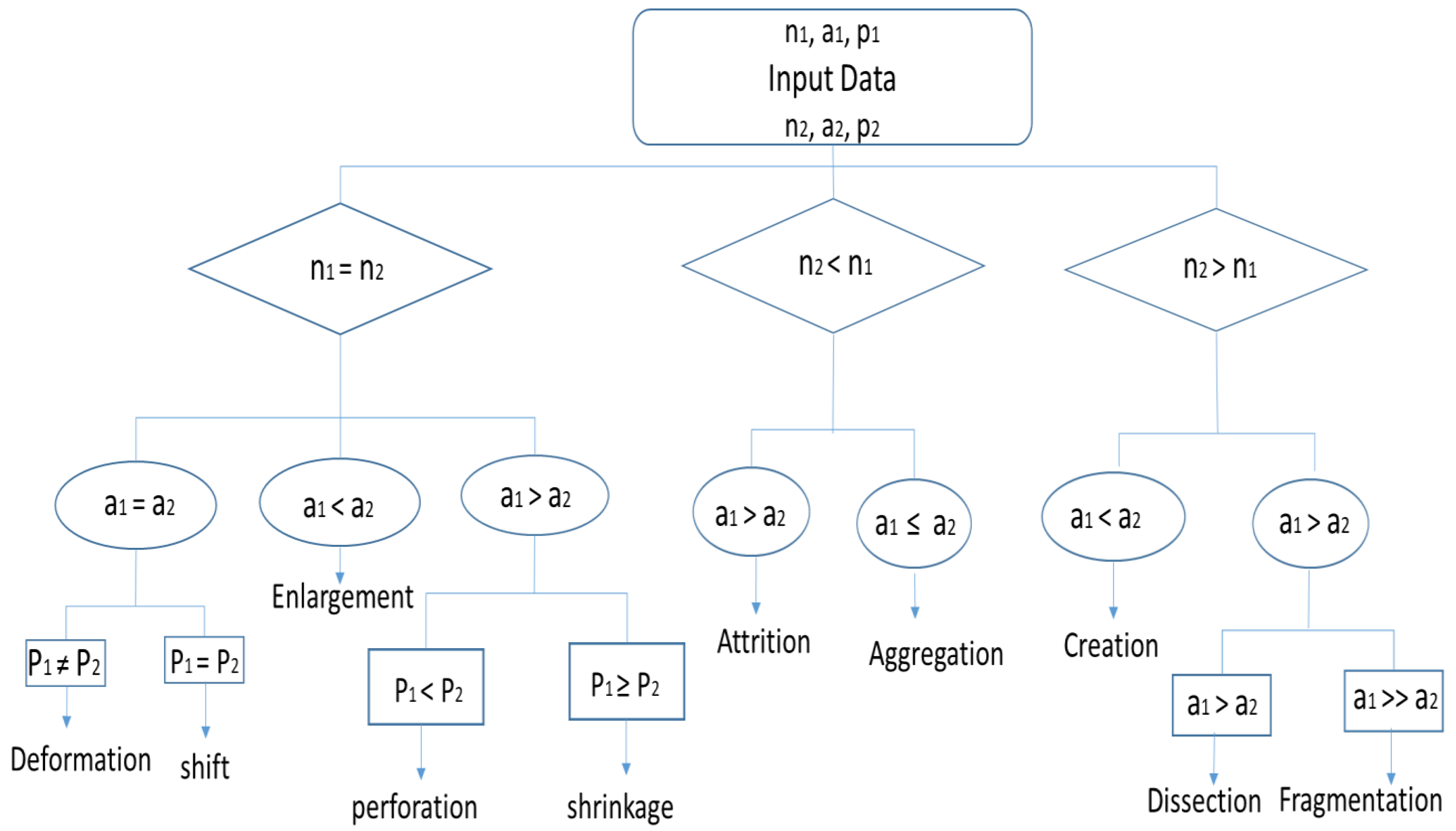
) were extracted and analyzed for each class and landscape level, eight-cell neighborhood rule, and non-sampling strategy [34]. The eight-cell neighborhood method uses eight cells adjacent to a center cell to determine the patches in the landscape. In the non-sampling strategy, each input map, LULC, to the model was considered as a separate landscape and the landscape change processes were extracted. The landscape change processes include deformation, shift, perforation, enlargement, shrinkage, attrition, aggregation, creation, dissection, and fragmentation, each of which is based on changes in three metrics including the number of patches, patch area, and patch perimeter (Figure 3). In this regard, the change processes over a period of time were determined using the decision tree algorithm to investigate the two LULC maps at times t1 and t2 and how the metrics are determined for each class of LULC. The landscape change processes in the GRB were finally extracted during the periods 1990–2000, 2000–2010, 2010–2020, and 2020–2040 (two scenarios).

3. Results

3.1. Analysis of LULC Maps

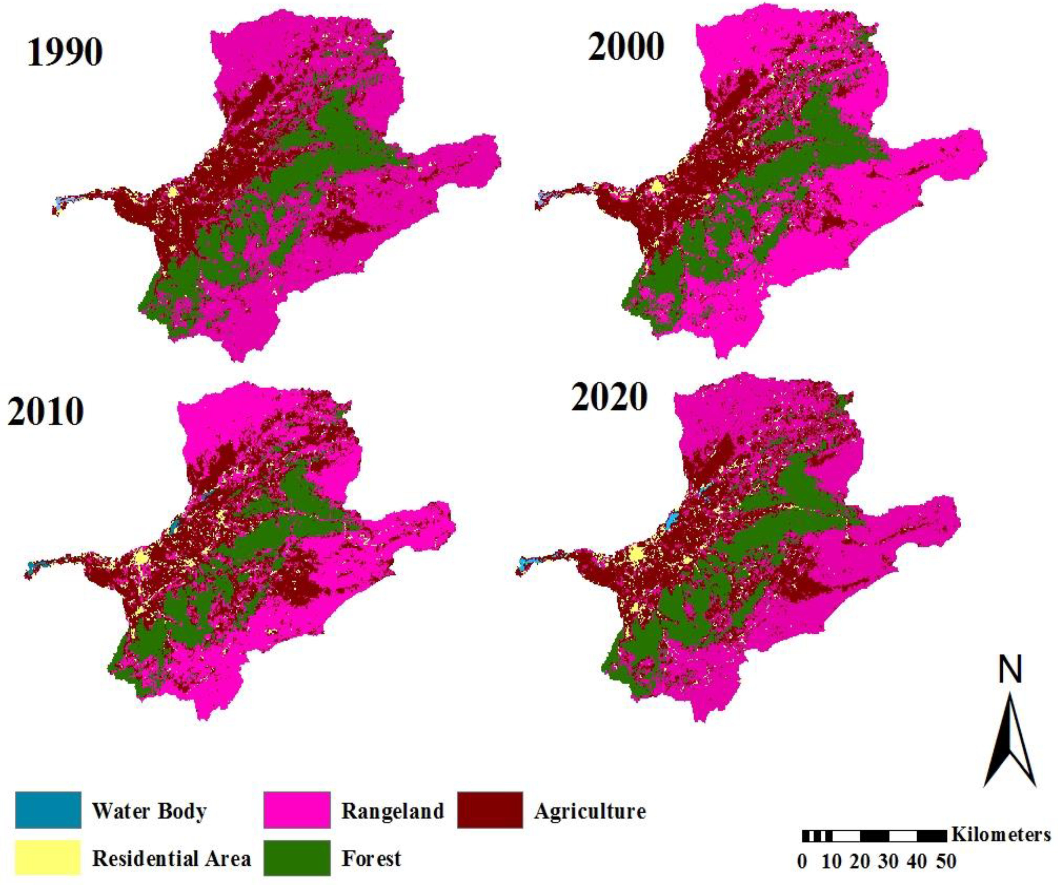
The generated LULC map of GRB during the studied years is shown in Figure 4. According to the maps, the forests class coverage reduced by 280 km² during the 1990–2020 period (3.7% of the total area), and the agricultural class coverage increased by 543 km² (7.2% of the total area). The dominant class was rangeland (51.5% in 1990 and 46% in 2020) in the study area. The rangeland class coverage increased by 61.6 km² during 1990–2000 but substantially decreased during 2000–2020 (reduced by 474.6 km²). During the first period (1990–2000), the forest area had been converted into rangeland by 27.5 km² and during the second period (2000–2010), the forest area had been turned into rangeland, agricultural lands, and residential areas by 42.3, 44.6, and 3.1 km², respectively.

To evaluate the accuracy of the prepared maps compared to the terrestrial reality maps, kappa coefficient values for maps of 1990, 2000, 2010, and 2020 were calculated yielding 0.81, 0.83, 0.86, and 0.95, respectively. The overall accuracy of these maps was also calculated yielding 87.21, 88.58, 90.56, and 96.46, respectively. The results indicated the high accuracy of the satellite-based LULC maps of the GRB.

3.2. Land Use Land Cover (LULC) Calibration and Validation

The results of the relationship between the effective variables and LULC changes for both calibration and validation periods using the Cramer correlation coefficient are presented in

Table 2. Result of Cramer statistic, revealing the degree of association between the explanatory variables with LULC changes during calibration and validation periods.

Variable	Calibration	Validation
DEM	0.3	0.3
Distance to forest	0.4	0.4
Distance to residential area	0.3	0.3
Distance to Agriculture	0.3	0.3
Distance to river	0.2	0.2
Distance to road	0.2	0.3
Empirical likelihood change	0.4	0.3

(all explanatory variables had a Cramer coefficient higher than 0.15).

The results of the evaluation of the multilayer perceptron (MLP) method for modeling transfer potential indicating accuracy (%), RMSE training, RMSE testing, and skill measure for calibration and validation periods are presented in

Table 3. Result of Multi-Layer Perceptron (MLP) method evaluation.

Period	Values
	Skill Measure	RMSE Test	RMSE Train	Accuracy (%)
Calibration	0.6	0.3	0.33	79.3
Validation	0.6	0.2	0.3	76.4

.

3.3. Prediction of LULC Map by 2040 Based on the Current Change Trend Scenario (Scenario 1)

The predicted LULC map of GRB in 2040 considering scenario 1 is depicted in Figure 5. The results of evaluating the accuracy of the LULC map based on statistical and visual criteria are presented in

Table 4. Result of LULC predicted map accuracy evaluation for 2020 in the Gorgan River Basin.

Year	ROC	$\frac{\mathit{H}\mathit{i}\mathit{t}\mathit{s}}{\mathit{F}\mathit{a}\mathit{l}\mathit{s}\mathit{e} \mathit{A}\mathit{l}\mathit{a}\mathit{r}\mathit{m}\mathit{s}}$	$\frac{\mathit{H}\mathit{i}\mathit{t}\mathit{s}}{\mathit{F}\mathit{a}\mathit{l}\mathit{s}\mathit{e} \mathit{A}\mathit{l}\mathit{a}\mathit{r}\mathit{m}\mathit{s}+\mathit{H}\mathit{i}\mathit{t}\mathit{s}+\mathit{M}\mathit{i}\mathit{s}\mathit{s}}$	Overall Kappa
2020	AUC = 0.9	0.7	14.3	0.8

. It should be noted that LULC was predicted by 2020 using the LCM model considering the LULC changes in 1990 and 2010. The existence of the terrestrial reality map in 2020 helped us to be able to accurately assess the accuracy of the model.

According to the LULC predicted map under scenario 1, the area of forest, agriculture, and rangeland with changes of -58.37, 35.80, and 8.28 km², respectively, would reach 1365, 2396, and 3481.2 km² by 2040 (

Table 5. Gorgan River Basin’s LULC classes area (km²) during the 1990–2020 period.

LULC Classes	1990		2000		1990–2000	2010		2000–2010	2020		2010–2020	2040 Current Trends	2040 Ecological Capability
	Area	%	Area	%	Area Changed	Area	%	Area Changed	Area	%	Area Changed	Area Changed	Area Changed
Forest	1702.9	22.6	1679.2	20.1	−23.6	1589.0	21.0	−90.2	1423.3	18.9	−165.7	−58.4	4.3
Agriculture	1817.2	24.1	1750.7	20.9	−66.5	2124.2	28.1	373.4	2360.2	31.3	236.0	35.8	−100.9
Rangeland	3885.9	51.5	3947.5	56.8	853.6	3529.7	46.8	−1209.7	3472.9	46.0	−56.8	8.3	96.6
residential areas	127.4	1.7	160.3	1.9	32.8	272.1	3.6	111.9	261.5	3.5	−10.6	10.6	0.4
Water body	14.7	0.2	10.45	0.13	−0.06	33.3	0.4	22.9	30.4	0.4	2.9	2.9	−0.7

).

3.4. Prediction of LULC Map by 2040 Based on the Landscape Ecological Capability Scenario (Scenario 2)

In scenario 2, the area of forests, agricultural lands, and rangelands with a change of 4.3, −100.9, and 96.6 km² would reach 1427.6, 2259.3, and 3569.5 km². The evaluation maps for each LULC capability are presented in Figure 6a–c. The final predicted map for 2040 based on scenario 2 is shown in Figure 6d.

Based on Figure 6a, the middle portion of the study area has the highest potential for forest growth. Agriculture capability has been scattered all around the area, especially in the northwestern part (Figure 6b). Most portions of the study area have a high potential for the development of rangelands, particularly in the northwest (Figure 6c). The final land capability map was obtained by integrating the ecological capability assessment maps of each LULC. Then, 10% of the most susceptible areas to change for each land use were selected to be changed by 2040. The selected areas were then added to the 2020 LULC map, so the final map of the ecological capability in 2040 based on scenario 2 was produced (Figure 6d). In this scenario, the landscape would face a change of 4.3, −100.9, and 96.6 km² for the area of forest, agriculture, and rangeland, respectively, by 2040 (Table 5).

3.5. Calculation of Metrics and Extraction of Landscape Change Processes

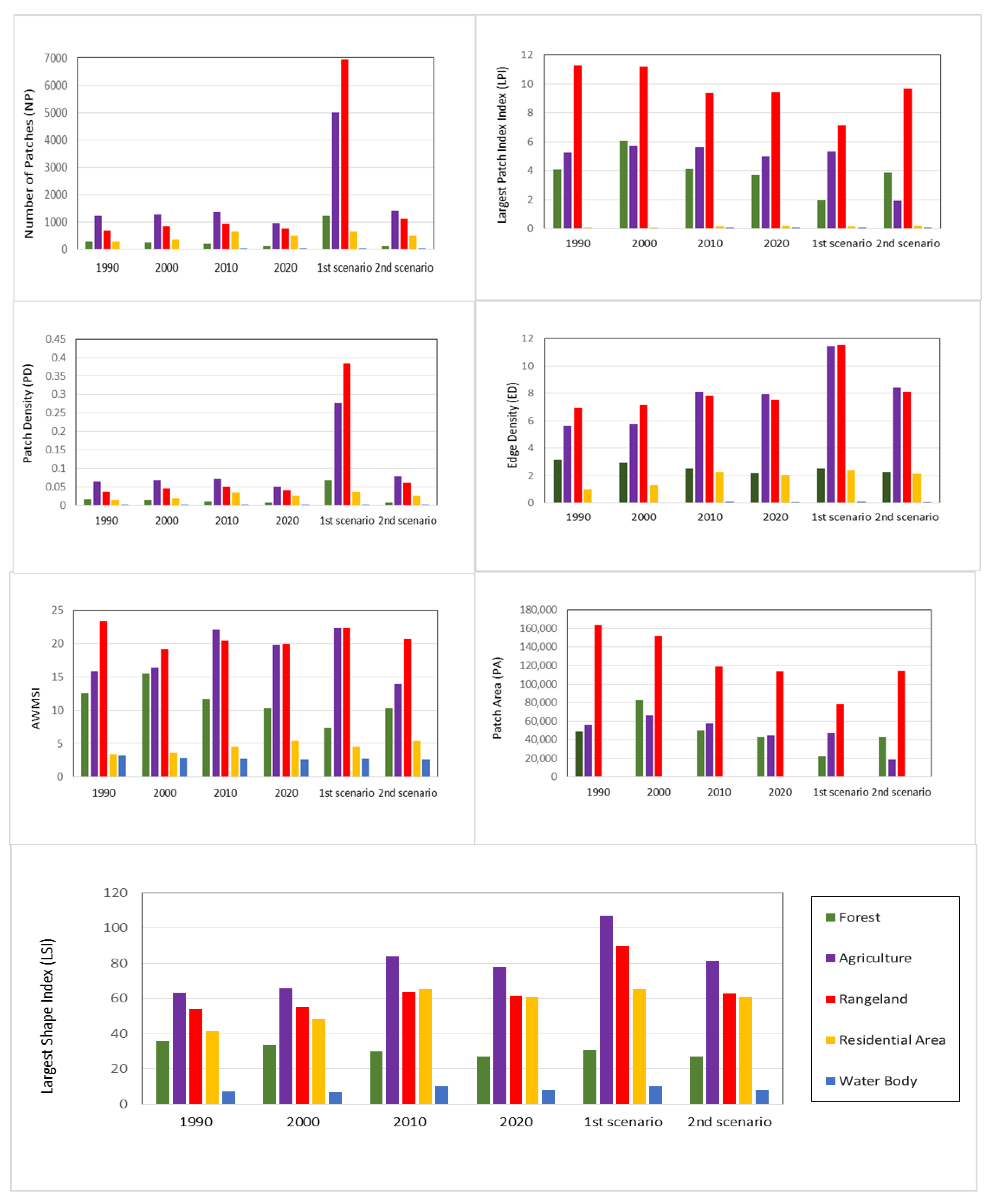
The results of landscape metrics during the studied years (1990, 2000, 2010, and 2020) and in two LULC maps based on scenarios 1 and 2 are presented in

Table 6. Result of landscape metrics at the landscape level.

Basin	Year	NP	PD	LPI	ED	LSI	PA	AWMSI
Gorgan River	1990	2484	0.1	11.3	8.4	29.7	108,825	18.7
	2000	2812	0.2	11.2	8.6	30.4	113,190	17.3
	2010	3236	0.2	9.36	10.4	36.7	82346	18.4
	2020	2391	0.1	9.40	9.9	34.9	74,349	17.6
	Scenario 1	13,888	0.8	7.2	14.0	48/0	55,126	18.9
	Scenario 2	3201	0.2	9.7	10.5	36.3	67,691	16.1

at the landscape levels and Figure 7 at the class levels.

Some landscape metrics including Edge Density (ED), Landscape Shape Index (LSI), Number of Patches (NP), and Patch Density (PD) showed an increasing trend from 1990 to 2010 and a decreasing trend from 2010 to 2020. The patch area (PA) and largest patch index (LPI) were reduced in both periods. The area-weighted mean shape index (AWMSI) showed a decreasing and increasing trend in the landscape during the studied periods. In addition, changes in ED, LSI, NP, and PD for the future conditions of the study area showed increasing trends in both scenarios, except that the intensity of this increase was higher in scenario 1. PA was shown to experience a decreasing trend in both scenarios, and the LPI would have a decreasing trend in scenario 1 and an increasing trend in scenario 2 (Table 6).

NP in the agricultural class increased from 1217 in 1990 to 1964 in 2020. This increasing trend of NP metric was also observed in residential areas. The number of forest and rangeland patches reduced from 291 to 271 and from 207 to 133, respectively, over a 30-year period. NP in scenario 1 would increase for all classes and in scenario 2 would increase for rangeland and agriculture and decrease for other classes.

The LSI of the forest class reduced from 36.1 to 21.4 during 1990–2020 and other classes increased during this period. Based on scenario 1, the percentage of changes in LSI for all classes would increase. Based on scenario 2, the rangeland and agriculture would increase. Other classes showed no significant trend in the LSI.

The value of PD in the GRB in all LULC classes except forest showed an increasing trend during the study years. In contrast, the largest patch index (LPI) during the 30-year period in most classes showed a decreasing trend. LPI for future conditions in scenario 1 for forests, rangeland, and residential area classes reduced compared to 2020, in the contrary, in scenario 2, a significant reduction was observed in the agriculture class compared to 2020.

AWMSI showed an increasing trend in agricultural land and residential area classes and a decreasing trend in other classes during the 30 years study period. The changes of this metric in future conditions showed, in scenario 1, a decreasing trend for forests and residential areas and an increasing trend for rangeland and agricultural lands. In scenario 2, however, this metric significantly decreased in the agriculture class by 2040.

ED decreased in the forests and increased in agriculture, rangeland, and residential areas. The value of ED, however, increased in both scenarios for all classes by 2040.

PA during the study period increased in the residential areas and opposite results were obtained in other classes. PA showed a decreasing trend in scenario 1 in forests, rangeland, and residential areas and an increasing trend in agriculture, in contrast, scenario 2 showed a decreasing trend only for agriculture.

Increases in NP during the study period were observed in all LULC categories other than forest and rangeland, indicating a trend toward increased fragmentation, shape irregularity, and complexity of patches in the LULC classes under consideration. The influence of human activities on landscape change in the GRB is shown by a growing trend of NP, LSI, and ED in the categories of agricultural, rangeland, and residential areas [43].

Zabihi et al. [43] noted that it is difficult to determine the dynamics of individual landscape patches. Therefore, it is advised to carry out the landscape change detection in a comprehensive spatial framework, which can be accomplished by using landscape change processes as a crucial idea offered by landscape ecology.

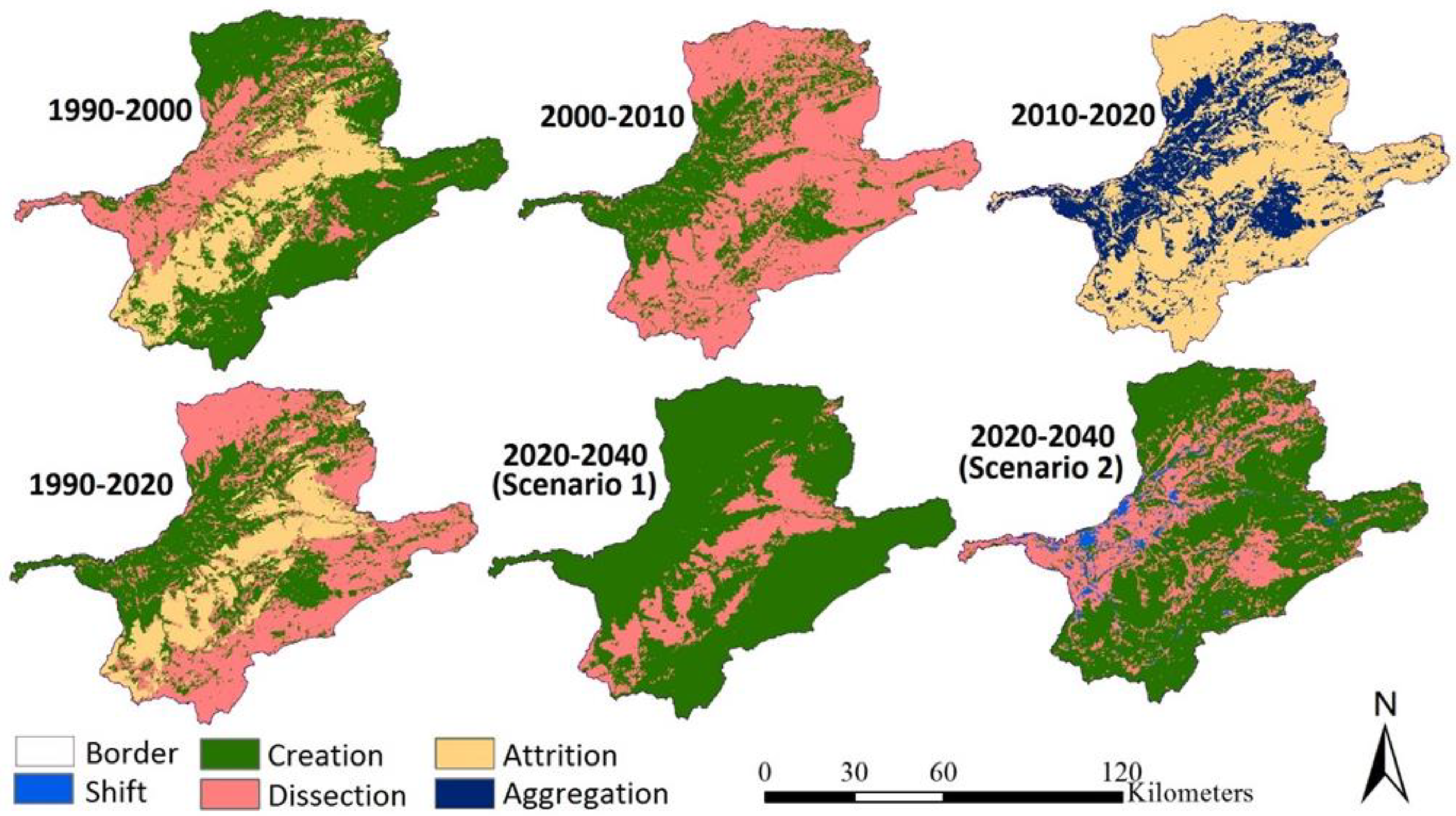
The results obtained from the extraction of the landscape change processes during the studied years for each LULC class in the GRB are presented in Figure 8 and

Table 7. Results of landscape metrics at the landscape level.

Basin	Classes	1990–2000	2000–2010	2010–2020	1990–2020	2020–2040 (Scenario 1)	2020–2040 (Scenario 2)
Gorgan river	Forests	attrition	dissection	attrition	attrition	dissection	creation
	Agriculture	dissection	creation	aggregation	creation	creation	dissection
	Rangeland	creation	creation	attrition	dissection	creation	creation
	Residential area	creation	creation	attrition	creation	creation	shift
	Water body	dissection	creation	attrition	creation	creation	creation

.

The findings of the landscape change process showed that attrition, creation, and dissection processes have taken place in the GRB during the study periods. In this regard, during the 30-year period, the process of attrition in the forests, the process of dissection in the rangeland, and the process of creation in agricultural lands and residential areas have occurred (Table 7).

4. Discussion

According to the study results, deforestation, reduction in rangeland lands, and development of agricultural lands and residential areas in GRB have occurred. Paudel and Yuan [44] indicated similar results for deforestation and development of the urban areas during the study period (1975–2006) in southern Minnesota in the USA.

The results showed that the highest conversion of classes in the study area during the study period (1990–2020) is related to changing forests to 157.6 km² of rangeland and 117.8 km² of agricultural lands, rangeland to 510.9 km² of agriculture, and agriculture to 75.4 km² residential areas. Deforestation during these years was mostly concentrated in the northeastern part of the GRB. This area is generally covered by high mountains with shallow and fine-textured soils. Severe soil erosion in loess soils and destructive floods are the most important factors leading to the destruction of forests in the northeastern part of the basin.

The human factor and population growth are the most important parameters affecting the change in the LULC in GRB. This result is consistent with the study results of Nor et al. [45] regarding the main cause of LULC change on a global scale. The continuous growth of agricultural lands to meet the food demands of society is another force causing land use change and deforestation. In this regard, one of the policies that can be proposed in the agriculture sector is comprehensive, scientific, and principled management to increase agricultural efficiency and production, without increasing the area under cultivation through modifying irrigation techniques and cultivation methods. Similarly, Statuto et al. [46] detected decreasing forests and developing agricultural lands in their studies.

LULC transfer potential modeling maps can be used to identify vulnerable and endangered areas, and accordingly, preserve and regenerate the forest area through the adoption of management measures such as the construction of enclosures and fencing against the danger of destruction.

According to the results obtained from calculating the Cramer correlation coefficient during the studied periods (1990–2010 and 2010–2020), the maximum value of the Cramer coefficient during calibration (1990–2010) and validation (2010–2020) periods related to distance from forests, which is due to its participation in various class conversion in the studied basin. The minimum value of the Cramer correlation coefficient in GRB belongs to the distance between the river and the road. Likewise, Joorabian Shooshtari et al. [30] achieved similar results in their study. This may be due to LULC changes occurring in the middle parts, which are away from rivers and roads. In addition to the above, the variable of elevation with the Cramer coefficient of 0.33 plays an important role in modeling transfer potential that has also been detected by Kavian et al. [12] in the Haraz Basin in Mazandaran province, Iran. It should be noted that in recent years the construction of summer houses and consequently the development of gardens in the northern aspects of the Alborz Mountains justify the effect of elevation on transfer potential and class conversion.

In scenario 1, reducing the area of forests and increasing the area of agricultural lands, rangelands, and residential areas indicate that the human factor would play an important role in changing the LULC of the GRB in the future. Therefore, it is necessary to make the proper decisions regarding LULC management through various measures such as forest conservation, afforestation, conservation of irrigated lands as well as rangelands, limiting agricultural development on the mountainous terrains, and construction of gardens in upstream rangelands that would result in sustainable management of the basin. Whereas in the second scenario (based on ecological potential), the area of forest, agricultural lands, and rangeland uses with a change of 4.3, −100.9, and 96.6 km² will reach 1427.6, 2259.3, and 3569.5 km².

The number of Patches (NP) in agricultural lands and residential areas in GRB increased, which caused fragmentation in the classes. Analysis of NP alone provides limited information due to the lack of consideration of cases such as area, distribution, or density [47]. However, the mentioned metric along with other metrics of the landscape can provide useful information [48].

Reducing Landscape Shape Index (LSI) in the forests showed a reduction of the spatial heterogeneity in the landscape [10,49]. In this regard, it is necessary to take appropriate measures to prevent the change in the configuration of the landscape in the classes directly affected by humans. Increasing PD in agriculture (1990 to 2010) and rangeland (1990 to 2020) classes indicated the conversion of these classes into smaller patches. This indicates an increase in fragmentation and spatial heterogeneity of agriculture and rangeland classes in GRB, which is consistent with the study of [50,51]. The largest patch index (LPI) in most classes was decreasing during the 30-year period, as also mentioned in the study of [52] in Arasbaran forests in Iran. Their study showed fragmentation in most classes. According to LULC predicted map, the increase in recreation and technological advancement that expands road, water, electricity, gas, and other facilities in the mountainous areas can be considered as the possible drivers of LPI reduction for forests, rangeland, and residential area. However, in scenario 2, a significant reduction was observed in an agriculture class, which could be due to environmental considerations and class change based on the ecological capability of the landscape.

The trend of AWMSI showed patch diversity, sensitivity to fragmentation, and complexity of LULC patch boundary with high values [42,44]. The decreasing trend of AWMSI in the classes indicated that the class patch is simpler with less spatial heterogeneity. The reason for this may be attributed to the increase in the area and aggregation of the mentioned LULC classes as well as residential area development in the study area.

Decreasing ED in forests and increasing ED in agriculture, rangeland, and residential areas indicated the complexity of the shape of LULC patches during the study period. Reducing ED by 31% in forest class during the 30-year study period revealed the simplification of forest patch edges [18], which can be due to unauthorized changes in the class patch edge.

According to the temporal determination of landscape change processes in GRB during the study period, the type of change processes that occurred during those periods was found to be different. The creation process underwent a change for the agricultural class. Over a 30-year research period, the GRB’s decreasing trend of NP and PA resulted in an attrition change process for the forest category. In our study periods for the agricultural category in the GBR, the recognized land change processes were creation. For rangeland, dissection was the examined alteration process from 1990 to 2020. The creation process of change was identified in residential areas.

5. Conclusions

Analysis of the results of landscape change processes indicated fragmentation and dissection of the landscape, especially in land uses under the direct human influence in the GRB. Thapa and Murayama [53] showed how human activities and urban growth in Nepal caused fragmentation in the landscape. Joorabian Shooshtari et al. [30], using Landscape indices, demonstrated that due to human interference, the overall landscape mosaics became heterogeneous, causing habitat fragmentation and increased shape complexity.

In this way, large patches became smaller due to human activities, indicating the destructive status in the studied basin. Due to the significant area of rangeland in the study area and the occurrence of the dissection process during the period 2000–2010, which is the starting point in the cycle of change processes, as well as the occurrence of the creation process for future conditions based on LULC predicted maps, taking protective measures and preventing LULC changes seem to be necessary. In addition, the continuation of the decreasing trend in the forest class could endanger the life of these valuable resources that should be considered as a warning by water and land managers.