Water Quality Prediction Based on LSTM and Attention Mechanism: A Case Study of the Burnett River, Australia

Abstract

Prediction of water quality is a critical aspect of water pollution control and prevention. The trend of water quality can be predicted using historical data collected from water quality monitoring and management of water environment. The present study aims to develop a long short-term memory (LSTM) network and its attention-based (AT-LSTM) model to achieve the prediction of water quality in the Burnett River of Australia. The models developed in this study introduced an attention mechanism after feature extraction of water quality data in the section of Burnett River considering the effect of the sequences on the prediction results at different moments to enhance the influence of key features on the prediction results. This study provides one-step-ahead forecasting and multistep forward forecasting of dissolved oxygen (DO) of the Burnett River utilizing LSTM and AT-LSTM models and the comparison of the results. The research outcomes demonstrated that the inclusion of the attention mechanism improves the prediction performance of the LSTM model. Therefore, the AT-LSTM-based water quality forecasting model, developed in this study, demonstrated its stronger capability than the LSTM model for informing the Water Quality Improvement Plan of Queensland, Australia, to accurately predict water quality in the Burnett River.

1. Introduction

Changes in water quality greatly affect ecosystem and human health. Prediction of water quality is the use of a long-term collection of water quality data to forecast possible water quality trend over a period of time for the future. It provides a scientific decision-making basis for assessing water environment in advance and preventing the large-scale occurrence of water pollution problems. Accurate water quality prediction plays an essential role in improving water management and pollution control. The goal of the Burnett Water Quality Improvement Plan of Queensland, Australia, is to manage the pollutant loads into the Burnett waterways and to help protect the Great Barrier Reef (GBR) region. Establishment of an effective and accurate water quality parameter prediction model is of great significance for improving the water quality of the Burnett River [1].

As the cost of hardware equipment related to water quality monitoring has been decreasing, it is possible to deploy a large-scale water quality monitoring sensors in rivers and lakes [2]. Water quality monitoring sensors automatically monitor parameters such as DO, pH, turbidity, and many other indicators. All indicators are recorded in the order of the monitoring time occurrence of the time series. In recent years, with the large-scale operation of water quality automatic monitoring stations, substantial data are being produced, and big data-driven water quality prediction models are receiving more and more attention in the field of water research. However, due to the variety in water quality indicators, the long period of water quality data collection, the correlation among the water quality indicators, the nonlinearity between water quality characteristics, and the volatility of the data, accurate and effective prediction of water quality has become a challenging issue. The current research hotspots mainly focus on how to improve the applicability and reliability of water quality prediction models [3].

River water quality exhibits characteristics such as seasonality and periodicity on macroscopic timescales, with nonlinearity and uncertainty [4]. River water quality parameters are not only affected by external factors, but also by the historical values of independent variables and random perturbations, and the selection of lagged terms and correlation variables is one of the factors affecting the prediction accuracy. Organic contaminants account for a large proportion of river water pollution. Organic pollution of rivers, due to the oxygen consumption from decomposition of contaminants, causes dissolved oxygen in water to decrease rapidly, consequently leading to deterioration of water quality. The self-purification ability of river water bodies decreases, resulting in serious damage to the ecosystem. Dissolved oxygen is a critical parameter for the pollution of river water, as well as an important indicator for whether the river water has the ability of self-purification. In the water environment, the growth of aquatic plants and animals cannot be separated from the appropriate amount of dissolved oxygen. In this study, the key parameter of DO for water quality evaluation is used as the target for model construction and prediction evaluation [5].

There are many traditional statistical techniques for water quality prediction [6], such as the autoregressive integrated moving average (ARIMA) method [7], and multiple linear regression (MLR) model [8,9]. However, water environment indicators are affected by many complex factors such as physical, chemical, and biological, and they have strong nonlinear characteristics. The above linear distribution-based models often fail to consider the influence of these factors in an integrated manner. In this study, water quality prediction uses traditional machine learning methods, including support vector regression (SVR) [10,11,12], artificial neural networks (ANN) [13,14,15], and other nonlinear methods. Singh et al. [13] proposed the use of ANN to predict water environment time series indicators. Barzegar et al. [16] used wavelet neural network (GWNN) to predict the salt concentration of the Aji Chay River in Northwest Iran. Through the calibration and verification of the model, the superiority of GWNN in water quality prediction is evident. ANN is also a powerful data-driven prediction model, which can well fit the nonlinear relationship between time series [17]. However, these methods still do not sufficiently learn the hidden relevant features in the time series, which significantly affect the prediction accuracy.

Currently, most water quality data belong to long correlation series data [18], and there may be some important events with long delays and intervals in the corresponding time series. It is difficult for traditional machine learning methods to fully use the available information with long historical observations. Recursive neural network (RNN) [19] is one of the deep learning methods capable of preserving and utilizing memory from previous network states [20]. RNN is very flexible in dealing with time series and capturing nonlinear relationships [21]. Nevertheless, it is difficult for the traditional RNN model to retain long-term dependencies among the variables due to the gradient vanishment [22]. Long short-term memory (LSTM) is a variant of RNN and can effectively alleviate the RNN network time delay and gradient vanishment [23] by implementing gating [24]. The interactive operation among these gates makes LSTM have sufficient ability to address the problem of long-term dependencies which general RNNs cannot learn, and it can balance the temporal and nonlinear relationship of data [25]. LSTM has been widely used in the prediction of water quality [26,27]. Ye et al. [28] combined all the water quality monitoring data of the rivers in Shanghai, used the LSTM model to predict and verify the main pollutant index, potassium permanganate index (COD), in the rivers, and proved that the prediction accuracy and generalization ability of the model outperformed the traditional RNN network model. Barzegar et al. [29] proposed a hybrid model combining LSTM and convolutional neural network (CNN) that outperformed single machine learning models including SVR, CNN, LSTM, and decision tree (DL) in predicting short-term water quality variables for the Small Prespa Lake in Greece. This shows that there is still much room for research based on LSTM to achieve high-precision water quality prediction, which can be explored in the direction of optimizing the internal structure of the network or combining with other methods [30,31]. LSTM lacks the ability to pay different degrees of attention to sub-window features, which may lead to some relevant information being ignored, and the important characteristics of time series cannot be valued.

In recent years, attention mechanisms [32,33] have been deployed in various tasks of natural language processing [34,35,36,37], including machine translation [38,39], syntactic analysis [40,41], and speech recognition [42,43]. We have applied the attention mechanism to effectively capture the more distant critical information and enhance the influence of the important characteristics on the prediction model by weighting the hidden layer elements at each timestep. Attention mechanisms have also been widely adopted in the field of time series analysis and forecasting [44,45]. Zhou et al. [46] proposed a short-term photovoltaic power forecasting based on LSTM neural network and attention mechanism to forecast short-term photovoltaic power generation in a time series manner. On this basis, we introduced the attention mechanism and developed an AT-LSTM model based on the LSTM model, focusing on better capturing the water quality variables. The DO concentration in the section of the Burnett River, Australia, was predicted using water quality monitoring raw data. Lastly, the prediction results were compared with the LSTM model. We aimed to achieve adaptive learning of long-term dependencies and hidden correlation features of multivariate temporal data to make river water quality predictions more accurate. The Burnett River was considered a case study to illustrate the applicability of the proposed AT-LSTM model.

2. Data Source and Pre-Processing

2.1. Study Area and the Data

The Burnett River is located in southeastern Queensland, Australia, and originates on the western slopes of the Burnett Range east of the Eastern Highlands in a subtropical climate. The river flows southwest to Eidsvold, then turns east at Mundubbera, and finally flows northeast through Gayndah and Bundaberg before entering the Pacific Ocean at Burnett Heads after 270 miles (435 km) of navigation. It has a catchment area of 12,440 square miles (32,220 square kilometers). The major tributaries are the Auburn and Boyne rivers and the Baramba River. The Burnett Basin has a population of approximately 94,100 residents. The primary land use is grazing (77%, 2,500,000 hectares), followed by forestry (12%, 405,000 hectares). Approximately 10,100 hectares of sugar cane, the largest area of dryland cultivation (approximately 81,000 hectares), irrigated cultivation (approximately 41,000 hectares), and horticulture (approximately 10,000 hectares) are located in the Burnett watershed. It also contains several impoundments, including Paradise Dam. The catchment has undergone extensive modifications over the past 40 years, including industrial and port development in the estuary. The data used for this study are water quality data from the Burnett River automatic monitoring sites, the locations and catchment boundaries of which are shown in Figure 1.

To ensure the reliability and applicability of the model, we used the monitoring data of the water quality collected from January 2015 to January 2020 in the Burnett River. The data are collected every half-hour and include five characteristics: water temperature (Temp), pH, dissolved oxygen (DO), conductivity (EC), chlorophyll-a (Chl-a), and turbidity (NTU). In this paper, the hourly water quality data with 39,752 characteristics and dissolved oxygen are used as the output variable.

Table 1. Descriptive statistics of the water quality time series.

	Temp (°C)	EC (uS·cm−1)	pH	DO (mg·L−1)	Turbidity (NTU)	Chl-a (ug·L−1)
Count	39,601	39,752	39,752	39,752	39,752	39,752
Mean	24.31	37,536.07	7.86	6.63	14.96	9.23
Standard deviation	3.69	13,618.6	0.69	0.98	44.77	28.93

shows the descriptive statistics of the data.

In this water quality dataset, the indicators of the water quality data are mainly used to assess the water quality of the river. The DO used in this experiment is a key indicator of water organic pollution, which can reflect the degree of water pollution. In addition to DO water quality indicator, there are some indicators that affect water quality such as pH, Temp, EC, Chl-a, and turbidity. The variation of DO in the study period is shown in Figure 2.

2.2. Missing Value Processing

Missing values of data are handled in two ways: (1) if only one indicator is missing in one monitoring, the data are filled in by linear interpolation; (2) if a monitoring value is missing continuously, the data of the monitoring moments are deleted to avoid large errors caused by artificial filling.

Linear interpolation [47] is a widely used interpolation algorithm in the field of mathematics and graphics. Linear interpolation of water quality data can effectively compensate for the missing data problem of time series data and improve the model effect.

Assuming that there are missing values $\left(x,y\right)$ between coordinates $\left(x_0,y_0\right)$ and coordinates $\left(x_1,y_1\right)$, we can obtain Equation (1):

$$\frac{y-y_0}{x-x_0}=\frac{y_1-y_0}{x_1-x_0},$$

(1)

where $x$ is known, and the value of $y$ is obtained as in Equation (2):

$$y=y_0+\left(x-x_0\right)\frac{y_1-y_0}{x_1-x_0}=y_0+\frac{\left(x-x_0\right)y_1-\left(x-x_0\right)y_0}{x_1-x_0}.$$

(2)

After interpolation, the dataset becomes a continuous time series of equal time intervals.

2.3. Water Quality Correlation Analysis

The multivariate time series build predictive models by analyzing historical time series data and correlations between individual factors [48]. For multi-element water quality time series data, different element features have different effects on water quality prediction. Multiple features need to be selected, and feature selection can reduce model training time, improve model efficiency, and make its generalization ability stronger.

Pearson correlation test [49] is used to determine the relevance of different features to the time-series features that need to be predicted. The Pearson correlation is mainly used to describe the degree of linear correlation between variables. The Pearson correlation coefficient is calculated as the quotient of the covariance $E\left(XY\right)-E\left(X\right)E\left(Y\right)$ of variable $X$ and variable $Y$ divided by the standard deviation of the two variables, as shown in Equation (3):

$${\rho }_{X,Y}=\frac{E(XY)-E(X)E(Y)}{\sqrt{E\left(X^2\right)-{(E(X))}^2}\sqrt{E\left(Y^2\right)-{(E(Y))}^2}},$$

(3)

where $\rho$ is the correlation coefficient of variable $X$ and variable $Y$, and its absolute value is equal to 1. A correlation coefficient of 1 indicates that the two variables are strongly positively correlated and Y increases as $X$ increases; a coefficient of −1 indicates that the two variables are strongly negatively correlated and $Y$ decreases as $X$ increases; a coefficient of 0 indicates that there is no correlation between the two variables.

In this paper, we used the Pearson correlation test for relevant multifactor water quality characteristics, and final test results are shown in

Table 2. Pearson correlation feature screening results of water quality time series.

	Temp	EC	pH	DO	Turbidity	Chl-a
Temp	1	−0.247	−0.153	−0.411	0.248	0.403
EC	−0.247	1	0.056	−0.091	−0.453	−0.301
pH	−0.153	0.056	1	0.430	−0.085	0.054
DO	−0.411	−0.091	0.430	1	0.053	0.209
Turbidity	0.248	−0.453	−0.085	−0.053	1	0.468
Chl-a	0.403	−0.301	0.054	0.209	0.468	1

.

According to Table 2, the main element characteristics related to the water quality prediction index DO are pH, Chl-a, and Temp. The water quality prediction of multiple elements mainly considers these factors as the input characteristics.

2.4. Outlier Detection

Water quality monitoring stations are often affected by environmental changes and instrument failures in the process of data collection, resulting in missing data and data anomalies, which can have a serious impact on the subsequent model predictions. In this experiment, the detected anomalous values are considered as missing values, and linear interpolation is used to complete the data. Usually, outliers can be identified with the help of graphical methods (box-line plots and normal distribution plots) and modeling methods (linear regression, clustering algorithms, and K-nearest neighbor algorithms). This experiment used the box-line plot method to identify outliers.

The box-line plot technique [50] actually used the quantile of the data to identify the outliers among them. The graph is a typical statistical graph, which is widely used in both academia and industry. The shape of the box-line plot is characterized as shown in Figure 3.

The lower quartile in Figure 3 refers to the value corresponding to the 25% quartile of the data (Q1), the median is the value corresponding to the 50% quartile of the data (Q2), and the upper quartile is the value corresponding to the 75% quartile of the data (Q3). The formula for the upper whisker is Q3 + 1.5(Q3 − Q1), and the formula for the lower whisker is Q1 − 1.5(Q3 − Q1), where Q3 − Q1 denotes the quartile difference. If a box-line diagram is used to identify outliers, the judgment criterion is that when the data value of a variable is greater than the upper whisker of the box line diagram or less than the lower whisker of the box line diagram, such a data point can be considered as an outlier.

2.5. Data Normalization

For the joint multifactor water quality time series data prediction, different water quality indicators often have different levels. In the subsequent water quality time series prediction process, different levels of elements seriously affect the accuracy of model predictions. In addition, in the process of model training, too large or too small input data can lead to problems such as model nonconvergence. To solve this problem, this paper used outlier normalization (min–max normalization) [51] to normalize the data. Outlier normalization scales the data on the basis of the ratio of the difference between the maximum and minimum values such that the range of variation of water quality data is maintained between 0 and 1. Normalization can alleviate the impact of different scales on model training. The normalization formula is shown in Equation (4):

$$X_{norm}=\frac{X-X_{min}}{X_{max}-X_{min}}{X}_{norm}=\frac{X-X_{min}}{X_{max}-X_{min}},$$

(4)

where $X$ is the original data, $X_{norm}$ is the normalized data, $X_{max}$ is the maximum value in the original data, and $X_{min}$ is the minimum value in the original data.

2.6. Time Series Conversion to Supervised Data

Converting time series data from unsupervised data to supervised data is required before using a time series prediction model for forecasting to facilitate the model by comparing the gap between the true and predicted values. The conversion of time series data to supervised data relies on sliding window interception of feature input values and target values to construct supervised data [52]. Figure 4 shows the specific process.

3. Theoretical Foundation and Model Construction

3.1. Long Short-Term Memory Neural Network

The LSTM neural network is a special recurrent neural network (RNN) [53] that is capable of learning long-term patterns. It was first proposed by Hochreiter and Schmidhuber [54]. It has been applied very well to a wide variety of problems and is now widely used. The LSTM network is suitable for processing and predicting time-series features with very long intervals and delays in the time series. The LSTM network is also effective in solving the gradient disappearance and gradient explosion problems that tend to occur in traditional recurrent neural networks.

The LSTM model has an input gate, an output gate, and a forget gate, which are used to modify the memory. The input gate and output gate are mainly used to control the input features and output contents, while the forget gate is mainly used to decide which memories in the memory unit should be retained and which memories can be forgotten, which can be described by the Equations (5)–(9). The structure of LSTM is shown in Figure 5.

$$\mathrm{Input} \mathrm{gate}: i_t=\sigma \left(W_i\cdot \left[h_{t-1},x_t\right]+b_i\right).$$

(5)

$$\mathrm{Forget} \mathrm{gate}: f_t=\sigma \left(W_f\cdot \left[h_{t-1},x_t\right]+b_f\right),\hspace{1em}{\tilde{C}}_t=\tanh \left(W_C\cdot \left[h_{t-1},x_t\right]+b_C\right).$$

(6)

$$\mathrm{Output} \mathrm{gate}: o_t=\sigma \left(W_o\left[h_{t-1},x_t\right]+b_o\right).$$

(7)

$$\mathrm{Long} \mathrm{memory}: C_t=f_{\mathrm{t}}\ast C_{t-1}+i_t\ast {\tilde{C}}_t.$$

(8)

$$\mathrm{Short} \mathrm{memory}: h_t=o_t\ast \tanh \left(C_t\right).$$

(9)

The $W$ matrix represents the parameter matrix of various gates and memory cells, $x$ represents the input values, $h$ represents the hidden state variables, which are mainly used to store and update the historical information, and $\sigma$ and $\tan \mathrm{h}$ represent the sigmoid activation function and the $\tan \mathrm{h}$ activation function, respectively. Once trained sufficiently, the LSTM model can extract features of complex time series information. On the basis of these effective features (hidden layer information from the LSTM model), the final fully connected layer is able to decode them into predicted values with reasonable accuracy.

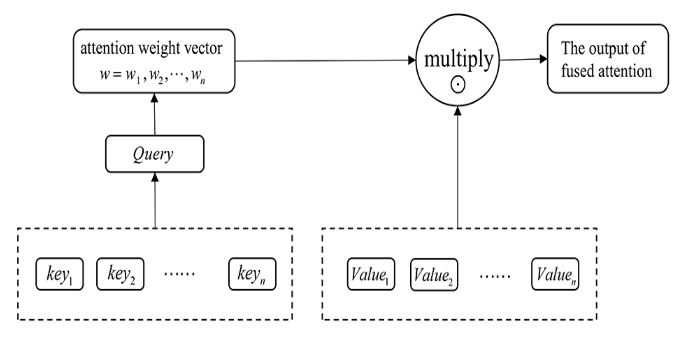
3.2. Attention Mechanism

The essence of the attention mechanism is that, for a given target, a weight coefficient is generated and multiplied with the input to identify which features in the input are important for the target and which features are not. To implement the attention mechanism, we consider the raw data of the input as $〈key,value〉$ pairs, and we calculate the similarity coefficient between $Key$ and $Query$. On the basis of the $Query$ in the given task in the target, we can get the weight coefficient corresponding to $Value$, and then multiply the weight coefficient with $Value$ to get the output. We use Q, K, and V to denote $Query$, $Key$, and $Value$; the formula for calculating the weight coefficient W is shown in Equation (10):

$$W=\mathrm{softmax}\left(Q{K}^T\right).$$

(10)

The attention weight coefficient $W$ is multiplied by $value$ using Equation (11) to obtain the output $a$ containing the attention.

$$a=attention(Q,K,V)=W\odot V=\mathrm{softmax}\left(Q{K}^T\right)\odot V.$$

(11)

The detailed structure of the attentional model is shown in Figure 6.

As we can see, the attention mechanism forms an attention weight vector by computing $〈key,value〉$, and then is multiplied by $value$ to get a new output incorporating attention. The attention mechanism has many applications in various fields of deep learning. However, it should be noted that attention is not a unified model, but only a mechanism that has different sources for $Query$, $key$, and $value$ in different application domains. This means that different domains have different implementation methods.

For the calculation of attention there are three steps: the first step is to calculate the similarity between the $Query$ and $key$ to get the weights, and the common similarity functions are dot product, splicing, and perceptron; the second step is to use a softmax [55] function to normalize these weights; the third step is that the weights are multiplied with the corresponding key value to get the final attention.

3.3. Model Establishment

In this research, we introduce an attention mechanism to the LSTM network and propose the AT-LSTM network model to process multivariate time series data. The main idea of the model is to reduce the effect of irrelevant factors on the results and highlight the impact of related factors by adaptively weighting hidden layer elements of the neural network, thus improving prediction accuracy. The model framework is shown in Figure 7, and the main components are the LSTM layer and the attention layer.

The model structures and main parameters are shown in

Table 3. Model structure.

Layers	Output Shape	Hidden Dimension
Input layer	(64, 100, 4)
LSTM	(64, 100, 100)	100
Dense	(64, 100, 100)	100
Activation (softmax)	(64, 100, 100)
Multiply	(64, 100, 100)
Flatten	(64, 10000)
Dense	(64, 1)	1
Activation (sigmoid)	(64, 1)

. The fully connected layer gets the normalized similarity weights via the softmax activation function. The weights are multiplied with the input layer to calculate the final attention. The flatten layer is used to “flatten” the input, which is to turn a multidimensional input into a one-dimensional one. The hyperparameter setting of the model affects its performance on water quality prediction to some extent. This paper sets the time window to 100 through a trial-and-error method, uses Bayesian optimization [56] for model hyperparameter optimization, and identifies relatively better hyperparameters and activation functions. The difference in the AT-LSTM model proposed in this study is the addition of the attention layer in comparison with the traditional LSTM model, while the other main structures are the same. In addition, the models were trained under the same hyperparameters, which helped us to compare the models. According to the above principle, the model learns on the basis of past fitting results, optimizes the water quality prediction by using the property of LSTM with memory, and finally outputs after activation through the fully connected layer.

The specific process of the comprehensive water quality data prediction algorithm proposed in this paper is as follows:

Step 1: Data cleaning. Before water quality prediction, the box-line plot technique in Section 2.4 is used to detect the abnormal values of water quality data, and the abnormal values are set to empty values. Then, the linear interpolation method in Section 2.2 is used to supplement the vacancy value

Step 2: Data enhancement. Firstly, the Pearson correlation test in Section 2.3 is used to select characteristics, the correlation analysis between different water quality parameters is performed, and the key characteristics related to the characteristic to be predicted are used as inputs to the model. Secondly, the sliding window technique in Section 2.6 with a window size of 100 is used to capture the trend of water quality variables. Thirdly, the min–max normalization in Section 2.5 is used to alleviate the impact of different characteristic scales on model training.

Step 3: Training model. The water quality data are divided into three datasets according to the ratio of 8:1:1: training, validation, and test set. In this study, the training set contained 31,802 hourly entries (from 1 January 2015 to 4 February 2019), the validation set contained 3975 hourly entries (from 4 February 2019 to 20 July 2019), and the test set contained 3975 hourly entries (from 20 July 2019 to 1 January 2020). We used the training set to fit data samples, the validation set to tune hyperparameters, and the test set to evaluate the predictive performance and generalization ability of the model. The algorithm flow chart is shown in Figure 8.

3.4. Performance Criteria

The water quality prediction is essentially a regression problem. In the present study, the mean absolute error (MAE), root-mean-square error (RMSE), and coefficient of determination (R²) were used to quantitatively evaluate the model prediction effect (as shown in Equations (12)–(14)). To reduce the randomness error of the algorithm, a random seed (random seed) was set during the experiment to ensure the consistency of the operation results.

$$\mathrm{RMSE}=\sqrt{\frac{1}{n}{\displaystyle \sum _{i=1}^n{\left({\widehat{y}}_i-y_i\right)}^2}},$$

(12)

$$\mathrm{MAE}=\frac{1}{n}{\displaystyle \sum _{i=1}^n\left.\left|{\widehat{y}}_i-y_i\right.\right|},$$

(13)

$${\mathrm{R}}^2={\displaystyle \sum _{i=1}^m{\left({\widehat{y}}_i-y_{\mathrm{mean} }\right)}^2}/{\displaystyle \sum _{i=1}^m{\left(y_i-y_{\mathrm{mean} }\right)}^2},$$

(14)

where $y_i$ is the measured value, ${\widehat{y}}_i$ is the predicted value, $y_{mean}$ is the mean value of $y_i$, and m is the number of test sets.

The RMSE is the square root of the MSE, a magnitude that is more intuitive. For example, if the RMSE is equal to 10, the regression effect can be considered to differ from the actual value by an average of 10. Its value ranges from zero to positive infinity; when it is equal to 0, it indicates a perfect model, with a larger the error denoted by a higher value. R² represents the fitting ability of the model; a closer value to 1 denotes a stronger fitting ability.

3.5. Experimental Environment

In this study, we used the Keras and Tensor-flow framework to provide water quality prediction with the following parameters: Intel i5-1140 CPU, 2.7 GHz frequency; Nvidia GTX 3050 GPU; 16 GB PC memory; Windows 10 64-bit operating system; Python version 3.9 development language; PyCharm Professional Edition 2021.3. To achieve the prediction of water quality in the Burnett River using AT-LSTM and LSTM models, we used the MSE as the loss function of the model and performed the calculations using the following standard equation:

$$\mathrm{loss}=\Vert Y-\widehat{Y}{\Vert }_2^2.$$

(15)

Both models were trained on the training set using the Adam optimizer [57] with a batch size of 64. To accelerate the convergence of the error, the backpropagation learning method was used. The validation set was used as an early stopping method to ensure that the model did not over-train.

4. Results and Discussion

4.1. Comparisons of One-Step-Ahead Forecast Using LSTM and AT-LSTM Models

This study aimed to analyze the differences between the AT-LSTM and LSTM models in multivariate time-series forecasting. The AT-LSTM and LSTM models used the past values of multivariate time series for one-step-ahead forecasting before performing multistep-ahead forecasting. The models used the same input data to predict the DO for the next hour. Figure 9a shows the comparison between the LSTM model and the AT-LSTM model when making predictions on the test set. From Figure 9a, we can see that the AT-LSTM model outperformed the LSTM model for water quality prediction for the Burnett River test set. The standard LSTM method performed less well, with an RMSE of 0.171 and R² of 0.918. After the introduction of the attention mechanism, RMSE and R² showed a reduction and an increase, respectively. This is because the attention layer in the model weighs hidden layer elements of the neural network of different moments, removes redundant information and noise in the time-series data, and highlights the influence of the relevant features on the prediction effect, thus improving prediction accuracy.

Detailed comparisons of predicted and actual values from the two models in the test set at the corresponding time allowed us to better understand the differences between the two such as shown in Figure 9b. In Figure 9b, the blue curve represents the actual values, and the orange curve indicates the predicted values from the modeling. Although LSTM can predict water quality changes, AT-LSTM’s predictions are less different from the actual values, indicating that AT-LSTM’s generalization abilities are stronger than those of LSTM.

Table 4. Performance indicators of the one-step-ahead DO prediction models for the testing dataset.

Models	RMSE	MAE	R2
LSTM	0.171	0.130	0.918
AT-LSTM	0.130	0.094	0.953

summarizes the performance of these models for the one-step-ahead DO prediction task in the monitoring sections. From the table, we can see that the method proposed in this paper shows significant improvements in the MAE, RMSE, and R² in comparison with LSTM. The R² of the AT-LSTM model increased from 0.918 to 0.953, and the RMSE and MAE of the AT-LSTM water quality prediction model had 23.9% and 27.7% reductions, respectively.

Figure 10 shows a box plot of the relative error percentage of each model in predicting DO. Clearly, the relative error distribution interval of the AT-LSTM model was smaller than that of the LSTM model. The attention mechanism allocated corresponding weights to the hidden layer elements of the neural network according to the different levels of importance of the hidden relevant features. Thus, with the same parameters used in the LSTM model, the AT-LSTM model could better fit the true value of DO, reduce the prediction error, and improve the accuracy and robustness of the model. The relative error percentage was calculated using Equation (16):

$${\delta }_t=\frac{\left|x_t-{\widehat{x}}_t\right|}{x_t}\times 100\%,$$

(16)

where $x_t$ is the actual value of the moment t, and ${\widehat{x}}_t$ is the predicted value of the moment t.

4.2. Comparisons of Multistep Forecasting Using the LSTM and AT-LSTM Models

To verify the prediction performance and generalization ability of AT- LSTM model, this study conducted DO water quality prediction experiments with different step lengths. The sliding window width was still set at 100. The prediction steps were 4–48 steps, i.e., the past 100 h of data to predict the future 4–48 h of water quality. A comparison of the prediction errors MAE, RMSE, and R² of the LSTM and AT-LSTM models for the test set is presented in

Table 5. MAE, RMSE, and R² for 4–48 h ahead prediction of LSTM and AT-LSTM.

Time (Hour)	RMSE		MAE		R2
	LSTM	AT-LSTM	LSTM	AT-LSTM	LSTM	AT-LSTM
4	0.229	0.201	0.178	0.152	0.853	0.887
8	0.271	0.238	0.212	0.178	0.794	0.841
12	0.295	0.228	0.232	0.173	0.757	0.854
16	0.297	0.229	0.234	0.171	0.753	0.853
20	0.317	0.254	0.248	0.191	0.719	0.820
24	0.335	0.263	0.267	0.194	0.686	0.806
28	0.365	0.346	0.280	0.256	0.626	0.664
32	0.374	0.357	0.292	0.271	0.607	0.644
36	0.367	0.355	0.282	0.269	0.623	0.647
40	0.406	0.374	0.315	0.288	0.538	0.608
44	0.446	0.378	0.348	0.288	0.443	0.601
48	0.422	0.405	0.333	0.312	0.501	0.541
Average errors	0.344	0.302	0.268	0.229	0.659	0.730

. Clearly, the MAE and RMSE values of the AT-LSTM model were smaller than those of the LSTM model in every step, and the R² of the AT-LSTM model was higher than that of the LSTM model at each step. The average values of MAE and RMSE of the total model decreased by 14.6% and 12.2% in comparison with LSTM, respectively, but the average R² increased by 10.8%. In terms of general trends, with the increase in the prediction step, the model prediction error also increased, being inferior to the prediction of the future 1 h.

Comparisons of the values of real and model-predicted DO, error plots, and residual histograms produced by the LSTM and AT-LSTM models for the next 48 h are presented in Figure 11 and Figure 12, respectively. They demonstrate the comparison of the reasonable precision of the 48 h ahead DO forecasts between AT-LSTM and LSTM. As shown in Figure 11 and Figure 12, although both the LSTM and AT-LSTM models accurately captured the trend of the DO content, the AT-LSTM model exhibited better prediction and stronger generalization than the LSTM model. The performance evaluation indices are presented in Table 5. The values of evaluation criteria produced by the LSTM model on the test set were as follows: R² = 0.501, MAE = 0.333, and RMSE = 0.422. On the other hand, the values of evaluation indicators produced by the AT-LSTM model on the same test set were as follows: R² = 0.541, MAE = 0.312, and RMSE = 0.405. This explains once again that the attention mechanism could improve the effectiveness and accuracy of the AT-LSTM model for prediction in multivariate time series.

4.3. Model Verification

A new independent dataset (Gregory River data) was used to verify the advantages of AT-LSTM over LSTM in the prediction performance of multivariate time series. The comparison of RMSE using the LSTM model and the AT-LSTM model for 1–12 h ahead prediction on the new dataset is shown in Figure 13. By comparing the variation of RMSE from LSTM and AT-LSTM models with the steps, it can be seen from Figure 13 that the RMSE of AT-LSTM predicted 1–12 h ahead on the new dataset was always lower than that of LSTM. This verifies that the AT-LSTM model proposed in this paper has more advantages than the traditional LSTM model in the prediction performance of multivariate time series. The above experimental results demonstrate that the developed deep learning AT-LSTM model outperformed the LSTM model in terms of prediction performance and could generalize the prediction capabilities outside the training station.

5. Conclusions and Future Work

With the rapid development of technology, gathering water quality data quickly evolves from manual collection to automatic monitoring, which makes the processing of water quality data of a large capacity and high frequency a reality. However, the traditional prediction method struggles to fully extract the true characteristics of water quality information; thus, the results of prediction cannot meet the needs of the actual application. It is urgent to develop a better water quality prediction method with higher accuracy. The AT-LSTM model proposed in this study incorporates the nonlinear mapping capability of the LSTM neural network and the feature weighting function of the attention mechanism, extracts the characteristic information of water quality data efficiently, and predicts the dissolved oxygen content of the Burnett River with significantly better accuracy than the LSTM model. In comparison with the standard LSTM model, the RMSE and MAE of the AT-LSTM water quality prediction model had 23.9% and 27.7% reductions, respectively, and it achieved a higher R² of 95.3% with better generalization performance. In practical application, the AT-LSTM model can be used to establish the water quality prediction and early warning platform of Burnett River, to sense the potential pollution risk of the river water in advance, send early warning reports, and conduct pollution retrieval. This AT-LSTM model can significantly improve the prediction ability of relevant departments on water environment risk, upgrade the passive water environment risk emergency treatment to automatic prediction, and provide early warning and active prevention, thus protecting the aquatic environment of the Burnet River and the Great Barrier Reef. Furthermore, the model proposed in this study can provide a reference for the construction of water quality prediction models of surface water bodies in other regions. Clearly, the AT-LSTM model has important application value and practical significance.

In addition, the AT-LSTM prediction model proposed in this paper has room for further optimization, and subsequent research work can be carried out from the following aspects. Firstly, this paper used only the water quality data of one monitoring point, whereby the water quality monitoring data of other sites in the study area can be added. The correlation of their geographical location can also be taken into account, such that not only the dimensionality of the data but also the amount of data will increase, thus enhancing the accuracy of water quality prediction and better improving the predictive performance of the model. Secondly, the feature screening method used in this study is a relatively simple Pearson correlation test algorithm which is a linear feature screening algorithm. For future studies, we will try data preprocessing and feature engineering methods, such as the use of nonlinear feature screening methods to find the impact of predictive indicators as more effective factors, hoping that the model’s prediction accuracy can be further improved.

References

1. Ho, J.Y.; Afan, H.A.; El-Shafie, A.H.; Koting, S.B.; Mohd, N.S.; Jaafar, W.Z.B.; Hin, L.S.; Malek, M.A.; Ahmed, A.N.; Melini, W.H.; et al. Towards a time and cost effective approach to water quality index class prediction. J. Hydrol. 2019, 575, 148–165. [Google Scholar] [CrossRef]
2. Zhou, J.; Wang, J.; Chen, Y.; Li, X.; Xie, Y. Water Quality Prediction Method Based on Multi-Source Transfer Learning for Water Environmental IoT System. Sensors 2021, 21, 7271. [Google Scholar] [CrossRef] [PubMed]
3. Liu, P.; Wang, J.; Sangaiah, A.K.; Xie, Y.; Yin, X. Analysis and Prediction of Water Quality Using LSTM Deep Neural Networks in IoT Environment. Sustainability 2019, 11, 2058. [Google Scholar] [CrossRef] [Green Version]
4. Duan, W.; He, B.; Chen, Y.; Zou, S.; Wang, Y.; Nover, D.; Chen, W.; Yang, G. Identification of long-term trends and seasonality in high-frequency water quality data from the Yangtze River basin, China. PLoS ONE 2018, 13, e0188889. [Google Scholar] [CrossRef] [PubMed]
5. Zhu, X.N.; Li, D.L.; He, D.X.; Wang, J.Q.; Ma, D.K.; Li, F.F. A remote wireless system for water quality online monitoring in intensive fish culture. Comput. Electron. Agric. 2010, 71, S3–S9. [Google Scholar] [CrossRef]
6. Koklu, R.; Sengorur, B.; Topal, B. Water Quality Assessment Using Multivariate Statistical Methods—A Case Study: Melen River System (Turkey). Water Resour. Manag. 2010, 24, 959–978. [Google Scholar] [CrossRef]
7. Ömer Faruk, D. A hybrid neural network and ARIMA model for water quality time series prediction. Eng. Appl. Artif. Intell. 2010, 23, 586–594. [Google Scholar] [CrossRef]
8. Kadam, A.K.; Wagh, V.M.; Muley, A.A.; Umrikar, B.N.; Sankhua, R.N. Prediction of water quality index using artificial neural network and multiple linear regression modelling approach in Shivganga River basin, India. Model. Earth Syst. Environ. 2019, 5, 951–962. [Google Scholar] [CrossRef]
9. Valentini, M.; dos Santos, G.B.; Muller Vieira, B. Multiple linear regression analysis (MLR) applied for modeling a new WQI equation for monitoring the water quality of Mirim Lagoon, in the state of Rio Grande do Sul—Brazil. SN Appl. Sci. 2021, 3, 70. [Google Scholar] [CrossRef]
10. Liu, S.; Tai, H.; Ding, Q.; Li, D.; Xu, L.; Wei, Y. A hybrid approach of support vector regression with genetic algorithm optimization for aquaculture water quality prediction. Math. Comput. Model. 2013, 58, 458–465. [Google Scholar] [CrossRef]
11. Candelieri, A. Clustering and support vector regression for water demand forecasting and anomaly detection. Water 2017, 9, 224. [Google Scholar] [CrossRef] [Green Version]
12. Granata, F.; Papirio, S.; Esposito, G.; Gargano, R.; De Marinis, G. Machine learning algorithms for the forecasting of wastewater quality indicators. Water 2017, 9, 105. [Google Scholar] [CrossRef] [Green Version]
13. Singh, K.P.; Basant, A.; Malik, A.; Jain, G. Artificial neural network modeling of the river water quality—A case study. Ecol. Model. 2009, 220, 888–895. [Google Scholar] [CrossRef]
14. Sundarambal, P.; Liong, S.-Y.; Tkalich, P.; Palanichamy, J. Development of a neural network model for dissolved oxygen in seawater. Indian J. Mar. Sci. 2009, 38, 151–159. [Google Scholar]
15. Li, C.; Li, Z.; Wu, J.; Zhu, L.; Yue, J. A hybrid model for dissolved oxygen prediction in aquaculture based on multi-scale features. Inf. Processing Agric. 2018, 5, 11–20. [Google Scholar] [CrossRef]
16. Barzegar, R.; Adamowski, J.; Moghaddam, A.A. Application of wavelet-artificial intelligence hybrid models for water quality prediction: A case study in Aji-Chay River, Iran. Stoch. Environ. Res. Risk Assess. 2016, 30, 1797–1819. [Google Scholar] [CrossRef]
17. Wu, G.-D.; Lo, S.-L. Predicting real-time coagulant dosage in water treatment by artificial neural networks and adaptive network-based fuzzy inference system. Eng. Appl. Artif. Intell. 2008, 21, 1189–1195. [Google Scholar] [CrossRef]
18. Hirsch, R.M.; Slack, J.R.; Smith, R.A. Techniques of trend analysis for monthly water quality data. Water Resour. Res. 1982, 18, 107–121. [Google Scholar] [CrossRef] [Green Version]
19. Medsker, L.R.; Jain, L. Recurrent neural networks. Des. Appl. 2001, 5, 64–67. [Google Scholar]
20. Cho, K.; Van Merriënboer, B.; Gulcehre, C.; Bahdanau, D.; Bougares, F.; Schwenk, H.; Bengio, Y. Learning phrase representations using RNN encoder-decoder for statistical machine translation. arXiv 2014, arXiv:1406.1078. [Google Scholar]
21. Hochreiter, S. The vanishing gradient problem during learning recurrent neural nets and problem solutions. Int. J. Uncertain. Fuzziness Knowl.-Based Syst. 1998, 6, 107–116. [Google Scholar] [CrossRef] [Green Version]
22. Bengio, Y.; Simard, P.; Frasconi, P. Learning long-term dependencies with gradient descent is difficult. IEEE Trans. Neural Netw. 1994, 5, 157–166. [Google Scholar] [CrossRef] [PubMed]
23. Pulver, A.; Lyu, S. LSTM with Working Memory. In Proceedings of the 2017 International Joint Conference on Neural Networks (IJCNN), Anchorage, AK, USA, 14–19 May 2017; IEEE: New York City, NY, USA, 2017; pp. 845–851. [Google Scholar]
24. Yu, Y.; Si, X.; Hu, C.; Zhang, J. A Review of Recurrent Neural Networks: LSTM Cells and Network Architectures. Neural Comput. 2019, 31, 1235–1270. [Google Scholar] [CrossRef] [PubMed]
25. Andersen, R.S.; Peimankar, A.; Puthusserypady, S. A deep learning approach for real-time detection of atrial fibrillation. Expert Syst. Appl. 2019, 115, 465–473. [Google Scholar] [CrossRef]
26. Wang, Y.; Zhou, J.; Chen, K.; Wang, Y.; Liu, L. Water quality prediction method based on LSTM neural network. In Proceedings of the 2017 12th International Conference on Intelligent Systems and Knowledge Engineering (ISKE), Nanjing, China, 24–26 November 2017; pp. 1–5. [Google Scholar]
27. Hu, Z.; Zhang, Y.; Zhao, Y.; Xie, M.; Zhong, J.; Tu, Z.; Liu, J. A water quality prediction method based on the deep LSTM network considering correlation in smart mariculture. Sensors 2019, 19, 1420. [Google Scholar] [CrossRef] [Green Version]
28. Ye, Q.; Yang, X.; Chen, C.; Wang, J. River water quality parameters prediction method based on LSTM-RNN model. In Proceedings of the 2019 Chinese Control and Decision Conference (CCDC), Nanchang, China, 3–5 June 2019; IEEE: New York City, NY, USA, 2019; pp. 3024–3028. [Google Scholar]
29. Barzegar, R.; Aalami, M.T.; Adamowski, J. Short-term water quality variable prediction using a hybrid CNN–LSTM deep learning model. Stoch. Environ. Res. Risk Assess. 2020, 34, 415–433. [Google Scholar] [CrossRef]
30. Baek, S.-S.; Pyo, J.; Chun, J.A. Prediction of Water Level and Water Quality Using a CNN-LSTM Combined Deep Learning Approach. Water 2020, 12, 3399. [Google Scholar] [CrossRef]
31. Sha, J.; Li, X.; Zhang, M.; Wang, Z.-L. Comparison of Forecasting Models for Real-Time Monitoring of Water Quality Parameters Based on Hybrid Deep Learning Neural Networks. Water 2021, 13, 1547. [Google Scholar] [CrossRef]
32. Bahdanau, D.; Cho, K.; Bengio, Y. Neural machine translation by jointly learning to align and translate. arXiv 2014, arXiv:1409.0473. [Google Scholar]
33. Luong, M.-T.; Pham, H.; Manning, C.D. Effective approaches to attention-based neural machine translation. arXiv 2015, arXiv:1508.04025. [Google Scholar]
34. Ma, F.; Chitta, R.; Zhou, J.; You, Q.; Sun, T.; Gao, J. Dipole: Diagnosis prediction in healthcare via attention-based bidirectional recurrent neural networks. In Proceedings of the 23rd ACM SIGKDD International Conference on Knowledge Discovery and Data Mining, Halifax, NS, Canada, 13–17 August 2017; pp. 1903–1911. [Google Scholar]
35. Gatt, A.; Krahmer, E. Survey of the state of the art in natural language generation: Core tasks, applications and evaluation. J. Artif. Intell. Res. 2018, 61, 65–170. [Google Scholar] [CrossRef] [Green Version]
36. Young, T.; Hazarika, D.; Poria, S.; Cambria, E. Recent Trends in Deep Learning Based Natural Language Processing [Review Article]. IEEE Comput. Intell. Mag. 2018, 13, 55–75. [Google Scholar] [CrossRef]
37. Galassi, A.; Lippi, M.; Torroni, P. Attention in Natural Language Processing. IEEE Trans. Neural Netw. Learn. Syst. 2021, 32, 4291–4308. [Google Scholar] [CrossRef]
38. Vaswani, A.; Shazeer, N.; Parmar, N.; Uszkoreit, J.; Jones, L.; Gomez, A.N.; Kaiser, Ł.; Polosukhin, I. Attention is all you need. Adv. Neural Inf. Processing Syst. 2017, 30, 5998–6008. [Google Scholar]
39. Britz, D.; Goldie, A.; Luong, M.-T.; Le, Q. Massive exploration of neural machine translation architectures. arXiv 2017, 1442–1451. arXiv:1703.03906. [Google Scholar]
40. Strubell, E.; Verga, P.; Andor, D.; Weiss, D.; McCallum, A. Linguistically-informed self-attention for semantic role labeling. arXiv 2018, 5027–5038. arXiv:1804.08199. [Google Scholar]
41. Clark, K.; Khandelwal, U.; Levy, O.; Manning, C.D. What does bert look at? an analysis of bert’s attention. arXiv 2019, arXiv:1906.04341. [Google Scholar]
42. Chorowski, J.; Bahdanau, D.; Cho, K.; Bengio, Y. End-to-end continuous speech recognition using attention-based recurrent NN: First results. arXiv 2014, arXiv:1412.1602. [Google Scholar]
43. Zeyer, A.; Irie, K.; Schlüter, R.; Ney, H. Improved training of end-to-end attention models for speech recognition. arXiv 2018, arXiv:1805.03294. [Google Scholar]
44. Song, H.; Rajan, D.; Thiagarajan, J.; Spanias, A. Attend and diagnose: Clinical time series analysis using attention models. In Proceedings of the AAAI Conference on Artificial Intelligence, New Orleans, LA, USA, 2–7 February 2018. [Google Scholar]
45. Tran, D.T.; Iosifidis, A.; Kanniainen, J.; Gabbouj, M. Temporal Attention-Augmented Bilinear Network for Financial Time-Series Data Analysis. IEEE Trans. Neural Netw. Learn. Syst. 2019, 30, 1407–1418. [Google Scholar] [CrossRef] [Green Version]
46. Zhou, H.; Zhang, Y.; Yang, L.; Liu, Q.; Yan, K.; Du, Y. Short-Term Photovoltaic Power Forecasting Based on Long Short Term Memory Neural Network and Attention Mechanism. IEEE Access 2019, 7, 78063–78074. [Google Scholar] [CrossRef]
47. Hipel, K.W.; McLeod, A.I. Time Series Modelling of Water Resources and Environmental Systems; Elsevier: Amsterdam, The Netherlands, 1994. [Google Scholar]
48. Zhang, Q.; Wang, R.; Qi, Y.; Wen, F. A watershed water quality prediction model based on attention mechanism and Bi-LSTM. Environ. Sci. Pollut. Res. Int. 2022, 29, 75664–75680. [Google Scholar] [CrossRef]
49. Lee Rodgers, J.; Nicewander, W.A. Thirteen Ways to Look at the Correlation Coefficient. Am. Stat. 1988, 42, 59–66. [Google Scholar] [CrossRef]
50. Chambers, J.M.; Cleveland, W.S.; Kleiner, B.; Tukey, P.A. Graphical Methods for Data Analysis; Chapman and Hall/CRC: Boca Raton, FL, USA, 2018. [Google Scholar]
51. Rathnayake, D.; Perera, P.B.; Eranga, H.; Ishwara, M. Generalization of LSTM CNN ensemble profiling method with time-series data normalization and regularization. In Proceedings of the 2021 21st International Conference on Advances in ICT for Emerging Regions (ICter), Colombo, Sri Lanka, 2–3 December 2021; pp. 1–6. [Google Scholar]
52. Shin, H.H.; Stieb, D.M.; Jessiman, B.; Goldberg, M.S.; Brion, O.; Brook, J.; Ramsay, T.; Burnett, R.T. A temporal, multicity model to estimate the effects of short-term exposure to ambient air pollution on health. Environ. Health Perspect. 2008, 116, 1147–1153. [Google Scholar] [CrossRef] [PubMed] [Green Version]
53. Salehinejad, H.; Sankar, S.; Barfett, J.; Colak, E.; Valaee, S. Recent advances in recurrent neural networks. arXiv 2017, arXiv:1801.01078. [Google Scholar]
54. Hochreiter, S.; Schmidhuber, J. Long Short-Term Memory. Neural Comput. 1997, 9, 1735–1780. [Google Scholar] [CrossRef] [PubMed]
55. Shen, T.; Zhou, T.; Long, G.; Jiang, J.; Pan, S.; Zhang, C. DiSAN: Directional Self-Attention Network for RNN/CNN-Free Language Understanding. In Proceedings of the AAAI’18: AAAI Conference on Artificial Intelligence, New Orleans, LA, USA, 2–7 February 2018; p. 32. [Google Scholar]
56. Snoek, J.; Larochelle, H.; Adams, R.P. Practical bayesian optimization of machine learning algorithms. Adv. Neural Inf. Process. Syst. 2012, 25. [Google Scholar] [CrossRef]
57. Kingma, D.P.; Ba, J. Adam: A method for stochastic optimization. arXiv 2014, arXiv:1412.6980. [Google Scholar]
Figure 1. Location of monitoring points and the extent of the watershed.
Sustainability 14 13231 g001
Figure 2. Variation of dissolved oxygen content in Burnett River.
Sustainability 14 13231 g002
Figure 3. Structure of box-line diagram.
Sustainability 14 13231 g003
Figure 4. Sliding window diagram.
Sustainability 14 13231 g004
Figure 5. Structure of LSTM.
Sustainability 14 13231 g005
Figure 6. Diagram of attention structure.
Sustainability 14 13231 g006
Figure 7. The framework of the proposed AT-LSTM model.
Sustainability 14 13231 g007
Figure 8. Flowchart of water quality prediction algorithm based on attention mechanism and LSTM.
Sustainability 14 13231 g008
Figure 9. (a) Comparison of the predicted DO values of LSTM and AT-LSTM models with measured DO values in the test period. Blue dots refer to the scatter plot of the measured and predicted DO value, while the black dashed line denotes a perfect match where “measured DO value = predicted DO value”. (b) Comparison of predicted DO values of LSTM and AT-LSTM models with actual DO values in the test period.
Sustainability 14 13231 g009
Figure 10. Error percentage box diagram of each model.
Sustainability 14 13231 g010
Figure 11. Line graph, residual histogram, and error plots for 48 h ahead forecasting using LSTM model on the test dataset.
Sustainability 14 13231 g011
Figure 12. Line graph, residual histogram, and error plots for 48 h ahead forecasting using AT-LSTM model on the test dataset.
Sustainability 14 13231 g012
Figure 13. RMSE for 1–12 h ahead prediction of AT-LSTM model and LSTM model on the new dataset.
Sustainability 14 13231 g013