Simulation of Land Use and Carbon Storage Evolution in Multi-Scenario: A Case Study in Beijing-Tianjin-Hebei Urban Agglomeration, China

Abstract

In considering regional sustainable development, optimizing the distribution of land use and land cover (LULC) and improving terrestrial ecosystem carbon storage (CS) have emerged as major concerns. In this study, considering the synergistic effect between LULC and CS, a coupling model (named MPI) that integrates Multi-objective Optimization (MOP) model, the Patch-generating Land Use Simulation (PLUS) model, and the Integrated Valuation of Ecosystem Services and Trade-offs (InVEST) model, was proposed to simulate the 2030 CS and explore its spatial-temporal characteristics in a Beijing-Tianjin-Hebei urban agglomeration (BTH). The MPI model, which combines the advantages of the above three models, can optimize the LULC structure, simulate the LULC distribution, and efficiently extract CS variation. The results indicated that: (1) LULC changes in BTH were mostly represented in transfers between cropland, forest, and grassland; (2) three different scenarios were simulated using the MPI model, named BAU (Business as usual), EDP (Ecological development priority), and EEB (Ecological and economic balanced). The simulation results of the three scenarios are in line with their respective goals, and the results are quite different; (3) cropland, water, and bare land, will be reduced, and the constant shrinking of water is a pressing issue that must be addressed; and (4) the EEB scenario balanced ecological services and economic rewards, increased the ecosystem carbon sink function, and is an efficient way to investigate “carbon neutrality”. The application of the MPI model is of reference value for exploring the optimal configuration of land resources.

1. Introduction

A significant part of the global carbon cycle is served by terrestrial ecosystems, which annually absorb an average of 2.5 Pg of carbon, or 25% of the emissions from fossil fuels [1,2,3]. The effects of global warming on the economy, environment, and resources, make it a severe problem for humanity today [4,5,6,7]. The increasing carbon storage (CS) is now thought to be the most practical, eco-friendly, and practical way, to reduce the greenhouse effect [7,8]. Some researchers have pointed out that land use and land cover (LULC) is one of the most important elements affecting ecosystems carbon sequestration [9,10,11], about 1.6 Pg of carbon emissions per year are attributable to LULC variations [12]. China is the top carbon emitter, and its rapid development over the past few decades has been accompanied by unreasonable territorial spatial planning that has caused CS to decline in the majority of areas. China is currently facing numerous challenges on its path to becoming carbon neutral [13,14]. Therefore, for future land resource allocation and ecosystem function optimization, it is essential to comprehend the synergistic relationship of LULC and CS and dynamically modify land use planning [15].

The combined measurement-statistics approaches, such as the forest census [16] and the bookkeeping model [17] employed in China to estimate forest carbon storage, have accurate results, and are extensively utilized to solve the problem of CS estimation. However, the actual measurement process is laborious and time-consuming. As an illustration, Tang et al. set 14,371 sample squares in advance to estimate the total carbon pool (89.27 ± 1.05 Pg) in China [18], making it challenging to use such methods to quickly obtain the evolution characteristics of CS. A number of process models have been developed based on a significant amount of measured experience and the use of remote sensing and geographic information system, such as the BIOME-BGC model [19] and the TEM model [20]. These process models have obvious advantages for CS evolution analysis, but their generality is weak due to the high number of parameters and tailored design for particular vegetation types [21]. The Integrated Valuation of Ecosystem Services and Trade-offs (InVEST) model was developed to solve the above problems and quickly realize the calculation of different carbon pools. It only requires the carbon density data to estimate and map the CS of terrestrial ecosystems. The InVEST model has been widely used in regional carbon sequestration and emission functional mismatch analysis [22], historical CS evolution [23], and future prediction [24]. Since CS estimation in the InVEST model is dependent on LULC data, acquiring accurate LULC historical and future simulation spatial patterns is the foundation for a reasonable CS analysis.

LULC simulation entails both distribution prediction and demand estimation. For future LULC prediction, the enhanced Cellular Automata (CA) model is usually used. The CA model is a discrete grid dynamics model that includes both space and state and can be used to model the dynamic process of complex systems [25]. Currently, there are various improved CA models, such as Logistic-CA [26], ANN-CA [27], CLUE-S [28], and FLUS [29]. However, these models are unable to explore the underlying driving mechanisms of LULC change, which results in low simulation accuracy. The Patch-generating Land Use Simulation (PLUS) model, which integrated a CA model with a patch-generating simulation strategy, contains two parts: the land expansion analysis strategy (LEAS); and an improved CA model [30]. Based on the spatial data of driving factors and LULC, the LEAS part uses a random forest algorithm to calculate the spatial growth suitability of each land use type. The results of the former are input into the CA model, which uses a descending threshold mechanism to determine the LULC distribution. The prediction of LULC demand is most widely based on the Markov model, which assumes that future trends are consistent with historical changes [31,32]. However, because of this, it is difficult for this model to consider the individual development characteristics of the different study area, especially the lack of consideration for future policy implementation [33]. The Multi-objective Optimization (MOP) model, which enables users to design different objective functions and constraints based on different development objectives and set the quantity demanded for each land use type separately, has been used in urban and ecological barrier area [34,35].

In summary, MOP is a “top-down” model for optimizing the quantitative structure of LULC, PLUS is a “bottom-up” spatial simulation function, and InVEST is a spatial-temporal CS evolution analysis approach. In order to conduct a multi-scenario simulation analysis of LULC and CS, here we proposed a MOP-PLUS-InVEST coupling model (MPI). To validate the three stated objectives of the MPI model: (1) more accurate land use target planning; (2) high accuracy patch-level LULC simulation; and (3) modelling and investigation of CS evolution. The Beijing-Tianjin-Hebei city agglomeration (BTH) was chosen. Our main goals are as follows: (1) explore the spatial-temporal characteristics of LULC; (2) conduct dynamic simulations of CS at the patch scale; and (3) evaluate CS at the regional scale. This is to solve the problem of coordinated and sustainable development of regional ecology and economy, and to assist government departments in formulating and adjusting land-use planning.

2. Materials

2.1. Study Area

The BTH city agglomeration (113°04′–119°53′ E, 36°01′–42°37′ N) (Figure 1) consists of 13 cities: Beijing, Tianjin, Shijiazhuang, Baoding, Tangshan, Langfang, Xingtai, Handan, Hengshui, Cangzhou, Qinhuangdao, and Chengde. It is located in the west of the Taihang Mountains and the east of the Bohai Sea, with the terrain gradually decreasing t from northwest to southeast. The climate of this area belongs to warm temperate continental monsoon climate. BTH is China’s political and economic center in the north, accounting for 9.4% of GDP and 2.2% of land area [36]. Rapid urbanization has resulted in major “urban illnesses” in this region. According to the BTH Coordinated Development Planning Outline (2015), the integration of ecological conservation and the construction of effective environmental protection regulations are critical for regional sustainable development.

Numerous scholars have conducted research on the LULC and ecological elements in BTH, and explored the optimal options for land planning in various scenarios [36,37,38,39,40]. For example, Yang et al.’s scenario analysis explored the sustainable development approach of BTH from the perspective of land use [36]. Wu et al. predicted the supply and demand balance of ecosystem services on the basis of land use analysis [37]. However, earlier research on the BTH lack the consideration of policy factors, resulting in poor pertinence. In addition, the CS estimation and dynamic of BTH remain under-researched. In addition, CS estimates and dynamics of BTH still need to be studied.

2.2. Datasets

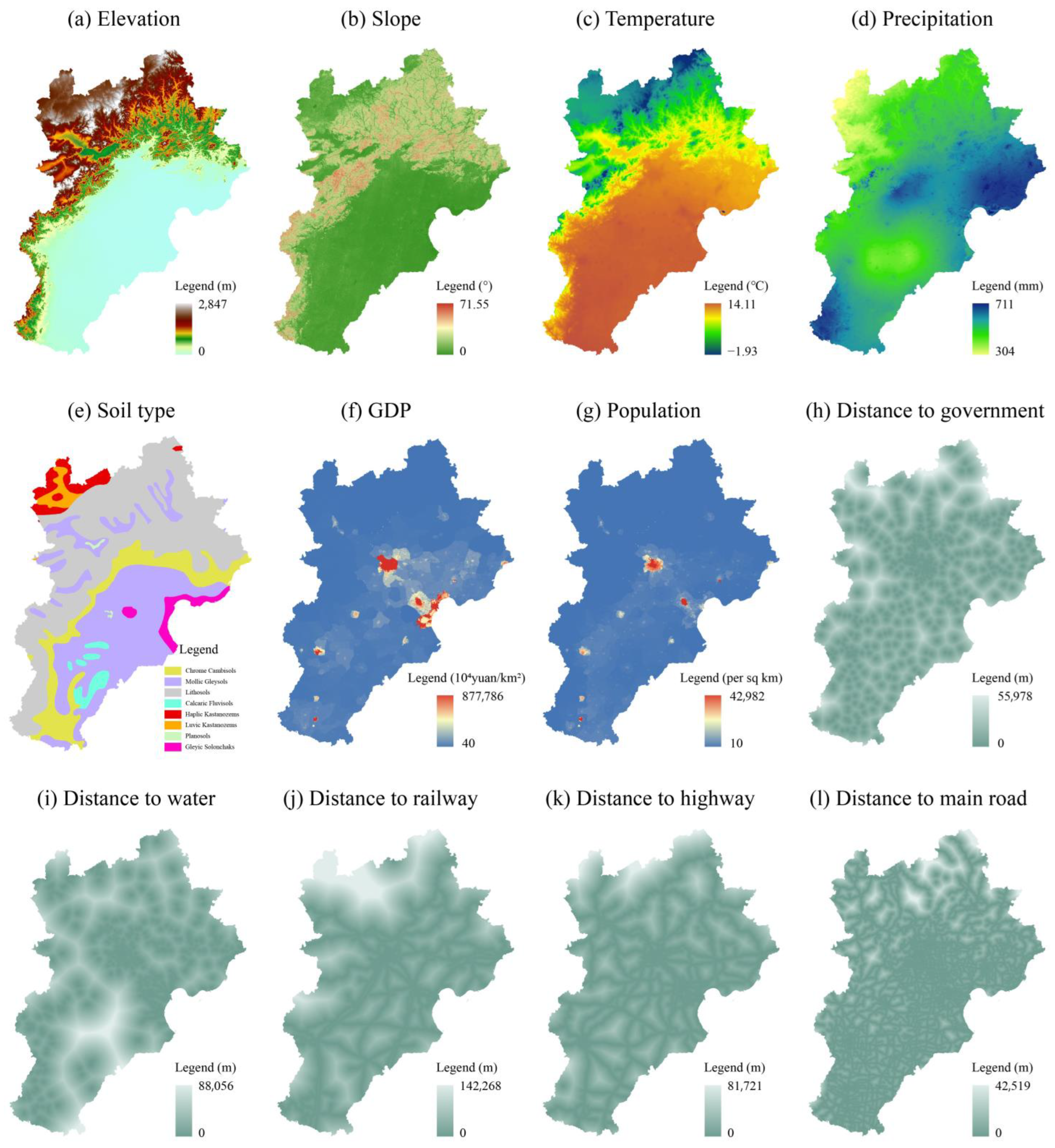
The primary sources of data for this analysis were LULC data from 2000 to 2020, environmental and socioeconomic drivers, accessibility factors, statistical data, policy planning documents, and data on carbon intensity, as shown in

Table 1. Presentation of data used in the study.

Category	Data Attribute	Time	Resolution	Source and Process
LULC	Land use and land cover	2000, 2010, 2020	30 m	GlobeLand30 (path/row:49/35, 49/40, 50/35, 50/40)
Carbon Density	Aboveground and belowground biomass carbon density	-	300 m	Temporally consistent and harmonized global maps form Spawn’s research
	Topsoil organic carbon density	-	1 km	GSOCmap (v1.5.0) from FAO
Natural drivers	Elevation, Slope	-	30 m	ASTER GDEM V3 from NASA (https://search.earthdata.nasa.gov/search?q=%20C1711961296-LPCLOUD, accessed on 20 May 2022), Slope data is calculated by ArcGIS
	Temperature and Precipitation	2000	0.5′	WorldClim v2.0
	Soil types	-	-	DSMW dataset from FAO
Socio-economic drivers	Population and GDP distribution	2015	1 km	China’s GDP and Population spatial distribution km grid dataset, from RESDC
Accessibility drivers	Distance to government residences, waters, highway, railway, primary way	2015	-	OpenStreetMap dataset, calculated in ArcGIS
Ecological conservation areas	Soil, water, windbreak and sand fixation functional area	2020	-	Boundary data of nature reserves in China, from RESDC
Statistical data	Yearbook, National Farm Product Cost-benefit Survey	2000–2020	-	Website of NBSC
Policy Planning Document	Planning for ecological protection, agricultural construction and national space	2016–2035	-	Website of Ministry of Natural Resources

. The LULC data is the GlobeLand30 dataset created by Chen et al. (http://www.globallandcover.com, accessed on 20 May 2022), with an overall precision of 84.61% and a Kappa coefficient of 0.80 [41]. Seven land use types are included in the GlobeLand30 dataset: cropland, forest, grassland, wetland, water, built-up, and bare land. A total of 12 potential drivers were chosen to investigate the mechanism of LULC and CS changes. These drivers including five natural, two socio-economic, and five accessibility factors. To create the restriction in the PLUS model, three ecological conservation reserve zones were extracted from the Chinese nature reserve border data given by the Resource and Environment Science and Data Center (RESDC, https://www.resdc.cn, accessed on 20 May 2022). Statistical information (yearbooks, National Farm Product Cost-benefit Survey) were from the National Bureau of Statistics of China (NBSC, https://data.stats.gov.cn/, accessed on 20 May 2022) and used to calculate and correct the ecosystem service valuation (ESV) and economic benefits per unit area in the study area. The policy planning documents were obtained from the Ministry of Natural Resources website (http://www.mnr.gov.cn/, accessed on 20 May 2022) and was used to set the parameters of the MOP model. The carbon density data consisted of aboveground, belowground biomass, and topsoil organic carbon density. The former two were obtained from the dataset published by Spawn’s et al. (https://doi.org/10.3334/ORNLDAAC/1763, accessed on 20 May 2022), which has global temporal consistency [42]. Topsoil organic carbon density was GSOCmap, (http://54.229.242.119/GSOCmap, accessed on 20 May 2022), a coordinated thematic map produced by the Food and Agriculture Organization of the United Nations (FAO) in collaboration with 110 countries worldwide [43].

3. Methods

3.1. MOP-PLUS-InVEST (MPI) Coupling Model

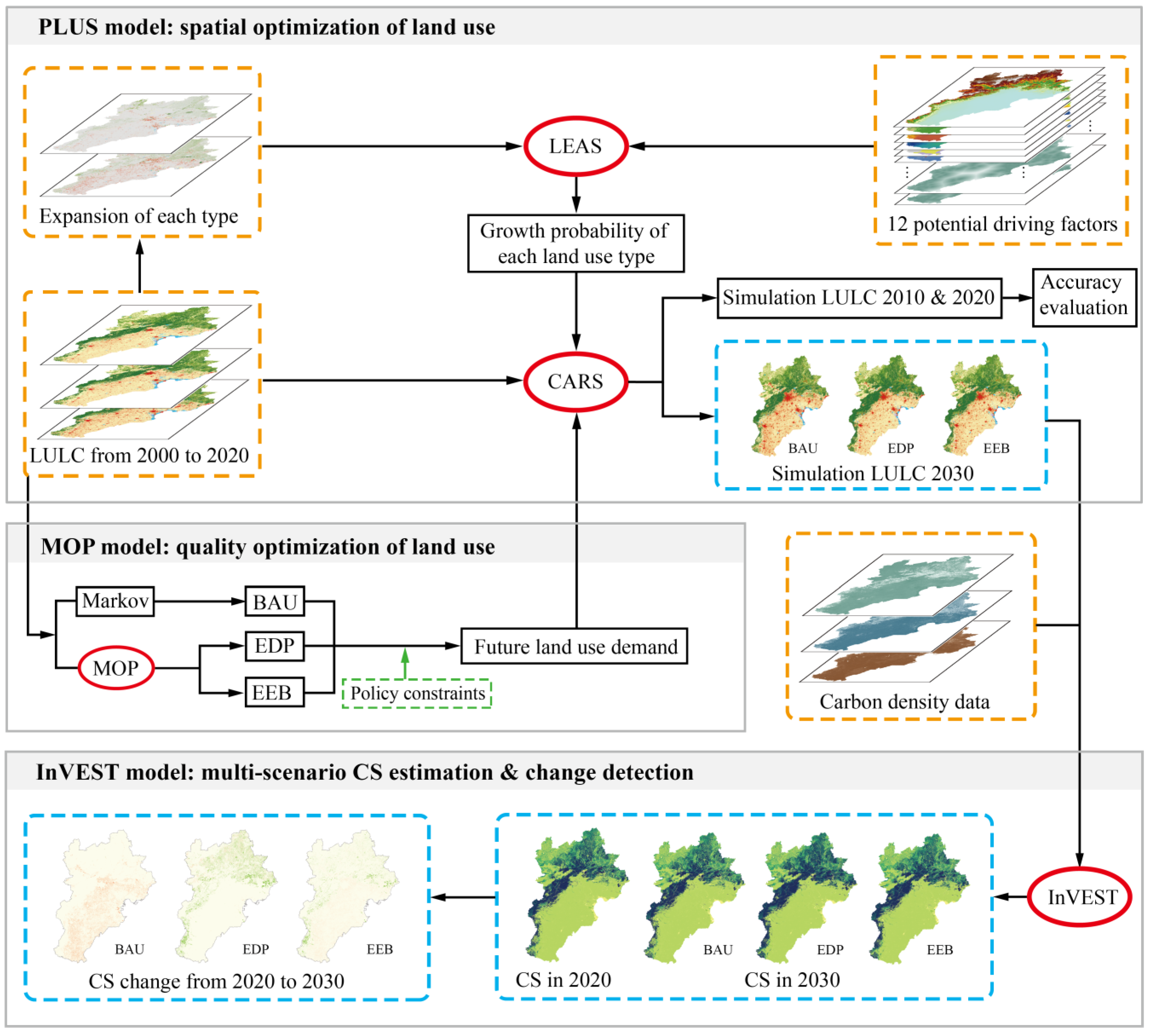
In this study, the MPI model was proposed based on the synergistic link between LULC and CS. The MPI model, as illustrated in Figure 2, is composed of three modules: the LULC structures (MOP) module, the LULC spatial simulation (PLUS) module, and the module for CS analysis (InVEST). Using the study area’s land use historical evolution and future planning, the MOP model was able to calculate land use demand under different development scenarios and offer import data for LULC simulation. The PLUS model was used to investigate the growth probability of each land type. The InVEST model was used to examine the evolution characteristics of CS.

3.2. LULC Quality Optimization by MOP

In the process of urbanization, the contradiction between economic development and the ecological environment has become increasingly prominent. The simulating of the future land conditions under various scenarios can be used as a guide for formulating relevant policies. We created three distinct scenarios: BAU (business as usual); EDP (ecological development priority); and EEB (ecological and economic balance). The MOP model was built on the lingo18.0 platform, with two objective functions and 15 constraint conditions.

3.2.1. Scenario Design and Objective Optimization

(1)

The BAU scenario is the creation of a baseline state of LULC based on the historical trend without the interference of additional factors. The Markov model was used to anticipate the land demand under the BAU scenario.

(2)

EDP is an ecological priority development scenario, which focuses on protecting the ecological environment and restore ecosystem functions. In short, the EDP scenario aims to maximize ecosystem service valuation (ESV), which is calculated in Equation (1).

$$f_{esv}\left(x\right)={\displaystyle {{\displaystyle \sum }}_{i=1}^7}es{v}_i·x_i$$

(1)

where $f_{esv}\left(x\right)$ is the sum of ESV provided by LULC. $x_i$ is the area of the $i^{\mathrm{th}}$ land use type, $i=1,2,···,7$, denoting cropland, forest, grassland, wetland, water, built-up, and bare land respectively. $es{v}_i$ is the ESV provided by the $i^{\mathrm{th}}$ land use type (yuan/km²) within an area unit. $es{v}_i$ was accessed using the method of equivalent value factor per unit ecosystem area [44]. The value of grain in the study area was corrected by combining the National Farm Product Cost-benefit Survey and yearbooks of Beijing, Tianjin, and Hebei. The $es{v}_i$ of seven land use types were 687,276.44, 3,631,767.53, 2,666,838.00, 8,915,740.77, 21,528,377.50, 0.00, and 34,278.13, respectively. In summary, the objective function of the MOP model under EDP scenario can be described as: $\max \left\{f_{esv}\left(x\right)\right\}$.

(3)

The EEB scenario represents the ecological environment and social economy development in a balanced manner, which aims to coordinate the improvement of economic benefits and the improvement of ecological functions by adjusting land use planning. The socio-economic benefits provided by LULC are calculated as shown in Equation (2).

$$f_{eb}\left(x\right)={\displaystyle {{\displaystyle \sum }}_{i=1}^7}e{b}_i·x_i$$

(2)

where $f_{eb}\left(x\right)$ is the socio-economic benefit of LULC. $e{b}_i$ is the socio-economic benefit per unit area of the $i^{\mathrm{th}}$ type (yuan/ km²). Based on the yearbooks of BTH in 2020 and the studies of Wang et al. [34] and Li et al. [35], $e{b}_i$ of seven land use types were calculated as 3,588,964.77, 874,521.30, 6,558,171.64, 52,231,514.45, 8,382,523.74 201,184,528.14, and 0.00. In summary, the objective function of the MOP model under EEB scenario can be described as: $\max \left\{f_{eb}\left(x\right),f_{esv}\left(x\right)\right\}$.

3.2.2. Constraint Conditions

(1)

The area constraint, means that the area is greater than zero, and the sum is equal to the area of study area.

$${\displaystyle {{\displaystyle \sum }}_{i=1}^7}{x}_i=\mathrm{215,583.97}$$

(3)

$$x_i>0$$

(4)

(2)

Population constraint, means that the number of people of built-up should be controlled within the target population.

$$d_P·x_6\le \mathrm{P}$$

(5)

where $d_P$ is the population density, $\mathrm{P}$ is the population number. Based on the 2000–2020 population statistics of Beijing, Tianjin, and Hebei and GM (1,1) model, $d_P$ was predicted to be 4209 persons/km² in 2030, and $\mathrm{P}$ was 116,282,700. According to the land use plans in BTH from2016 to 2035, the population of the study area will be controlled to around 122,100,000. Thus, $\mathrm{P}$ was set to the average of the above two (i.e., 119,191,350) in this study.

(3)

Forest cover constraint. According to the land use plans in BTH from 2016 to 2035, the forest cover in study area will reach more than 45% in 2030. Forest cover was calculated with the ecological green equivalent method, which refers to the photosynthesis per unit area of forest land as a green equivalent and has been shown to measure the ecological function of terrestrial ecosystems [34]. According to Li et al., the weighting coefficients for cropland, grassland, and forest are 0.46, 0.49, and 1, respectively [45]. The constraint of forest cover can be expressed as:

$$0.45\times x_1+x_2+0.49\times x_3\ge \mathrm{215,583.97}\times 45\%$$

(6)

(4)

Cropland area constraint, means that for ensuring national and regional food security, the food production of cropland should meet regional demand:

$$x_1·f_3·f_4·f_5\ge \mathrm{P}·f_1·f_2$$

(7)

where $f_1$ is per capita grain consumption (kg). $f_2$ is the regional food self-sufficiency rate, $f_3$ refers to the unit area yield of grain crops (kg/km²), $f_4$ is the proportion of grain crops grown, and $f_5$ means the replanting index. $f_1$ was set to 517 according to Xin et al.’s study on China’s food demand [46]. Hebei Province is a grain base in North China, and the grain production in BTH should at least meet the requirement of self-sufficiency, so $f_2$ was set to 100%. In accordance with the yearbooks and the GM (1, 1) model, $f_3$ and $f_4$ were set to 735,768 and 78.75%, respectively. According to a related study by Li et al. on the Yellow River and Huaihe River Basin [47], $f_5$ were set to 1.12.

In addition, on the basis of preserving high-quality cropland, implementing the project of returning farmland to forest and grassland in low-yielding areas is the main measure to manage cropland. In this study, the permanent basic farmland area (67,601 km²) was set as minimum, and the arable land area in 2020 (104,477.76 km²) was set as maximum:

$$\mathrm{67,601.00}\le x_1\le \mathrm{104,477.76}$$

(8)

(5)

Forest land area constraint. According to the Master Plan for the Major Projects for the Protection and Restoration of National Key Ecosystems (2021–2035) issued by the Chinese government in 2020, a strategic ecological protection pattern named “two screens and three belts” is proposed, to promote the construction of the northern sand control belt system. Therefore, the forest area was set to grow faster than the BAU scenario (42,160.91 km²) in the next decade. In summary, the constraint on the area of forest land can be expressed as:

$$x_3\ge \mathrm{42,160.91}$$

(9)

(6)

Grassland area constraint. The grassland has been relatively stable since 2000, and the interconversion of grassland, cropland, and forest, occurs frequently, reserving a part of space for landscape diversity and urban construction. In this study, the grassland area in 2020 (38,126.48 km²) was used as the basis, and the area change was controlled within 5%, which can be expressed as:

$$\mathrm{38,126.48}\times 95\%\le x_3\le \mathrm{38,126.48}\times 105\%$$

(10)

(7)

Built-up area constraint. According to the government plan, the construction land area per capita in BTH will be about 130 m² in 2030. At the same time, the growth of construction land will be strictly restrained in the future and its expansion will slow down. Thus, the built-up land was designed to be smaller than the built-up land area under the BAU scenario (33,240.51 km²):

$$P\times 130\times {10}^{-6}\le x_3\le \mathrm{33,240.51}$$

(11)

(8)

Water and wetland area constraint. Water and wetland are important ecological lands. At present, the local government has introduced policies such as returning farmland to wetlands, which will reduce the rate of degradation of water and wetland and rebuild ecological land in some nature reserves. So, the area of water and wetland under the BAU scenario was used as the lower limit and the average value in 2000–2020 was used as the upper limit:

$$476.69\le x_4\le 703.74$$

(12)

$$3635.73\le x_5\le 3839.50$$

(13)

(9)

Bare land area constraint. The pre-construction of the Xiong’an New Area in Hebei and the abandonment of a large amount of old industrial and mining land have increased the area. Considering that the bare land may be reclaimed in the future, the area in 2020 and 2000 were used as the upper and lower limits:

$$71.26\le x_5\le 232.30$$

(14)

(10)

Key ecological function constraint. In the latest ecological protection strategy, water conservation and soil preservation functions are given priority attention. The service values of “hydrological regulation” and “soil conservation” and total ESV in 2030 should be higher than those in 2020:

$$\begin{gathered} \mathrm{46,275.47}\times x_1+\mathrm{662,139.15}\times x_2+\mathrm{516,742.76}\times x_3+\mathrm{4,152,795.06}\times x_4+\mathrm{17,522,978.39}\times x_5+ \\ 5141.72\times x_7>\mathrm{120,901,993,150.47} \end{gathered}$$

(15)

$$\begin{gathered} \mathrm{176,532.35}\times x_1+\mathrm{432,475.70}\times x_2+\mathrm{324,785.25}\times x_3+\mathrm{395,912.36}\times x_4+\mathrm{159,393.29}\times x_5+ \\ 3427.81\times x_7>\mathrm{49,905,422,566.24} \end{gathered}$$

(16)

$$\begin{gathered} \mathrm{687,276.441}\mathrm{}\times x_1+\mathrm{3,631,767.53}\times x_2+\mathrm{2,666,838}\times x_3+\mathrm{8,915,740.765}\times x_4+\mathrm{21,528,377.5}\times x_5+ \\ \mathrm{34,278.13}\mathrm{}\times x_7>\mathrm{412,993,453,382.733} \end{gathered}$$

(17)

3.3. LULC Spatial Simulation by PLUS

The PLUS model is developed by Liang et al. of China University of Geosciences (Wuhan) [30]. Studies have shown that the PLUS model has the ability to simulate the patch-level evolution of land use landscapes [26,48,49]. In order to enhance the dependability of LULC simulation, the driving factors, LULC transfer rule, neighborhood weights, and space restriction, were set in the PLUS model.

3.3.1. Driving Factors

To exploit the suitability of land use types for growth, five natural drivers, two socio-economic drivers, and five accessibility factors, were chosen in this study (Figure 3).

3.3.2. Transfer Rule

The mechanism of transfer rule is to convert one land use type to other types. Under the general rule of LULC change, it is generally difficult to transfer built-up to other land use types, and it is reasonable for construction land to be converted to bare land in the short term. With a series of governance initiatives, the transfer of water and wetland to non-ecological land (i.e., cropland and built-up) should be strictly controlled.

3.3.3. Neighborhood Weights

Neighborhood weight ranges from 0 to 1, and the larger the value, the easier to assimilate the neighborhood. This parameter was calculated based on the ratio of the expansion area to the total expansion area of each land use type from 2000 to 2020. The neighborhood weights of the seven land use types were 0.178, 0.193, 0.247, 0.007, 0.036, 0.333, and 0.007, respectively.

3.3.4. Space Restriction

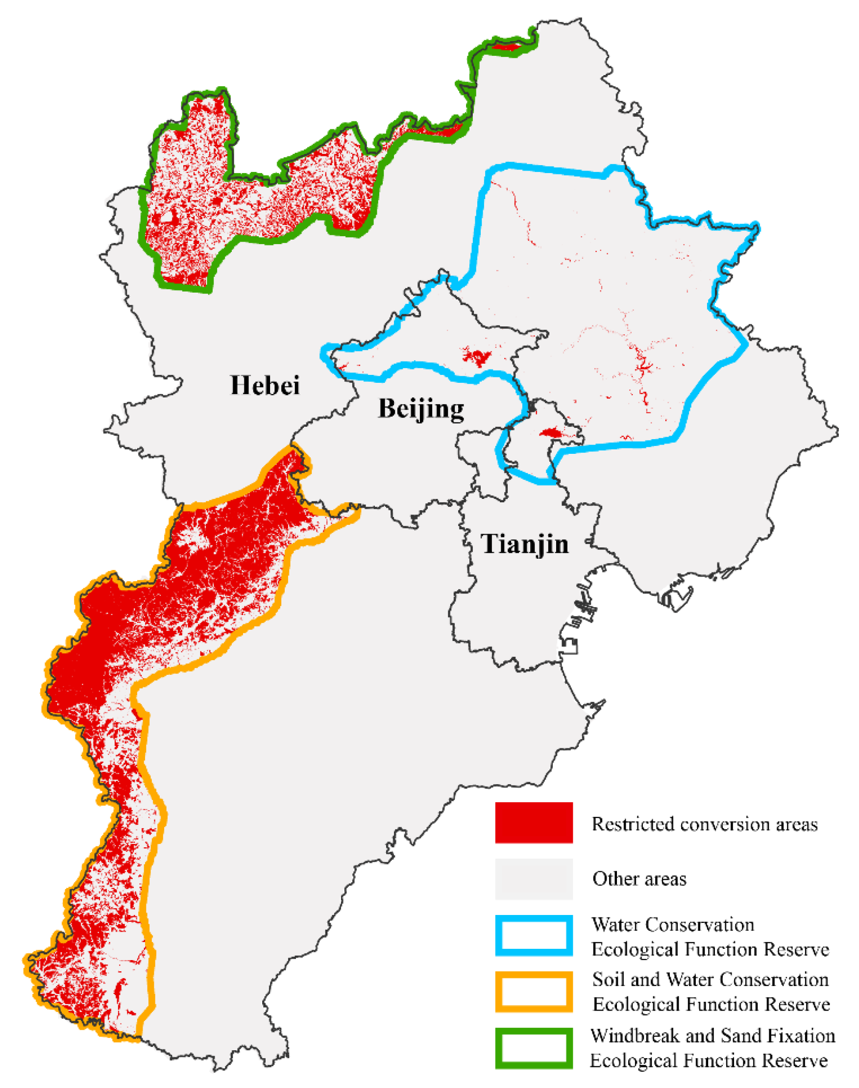
In the “two screens and three belts” ecological pattern, the study area includes the Taihang Mountain Ecological Function Reserve (soil and water conservation), the Beijing-Tianjin Water Conservation Ecological Function Reserve (water conservation protection), and the North of Yinshan Mountains-Hunshendake Sand Ecological Function Reserve (windbreak and sand fixation). Therefore, the following principles were formulated: within the scope of ecological protection areas, the transfer of land use types carrying key ecological functions is prohibited (Figure 4). For example, the water and wetland in the water conservation reserve were not allowed to be converted.

3.4. CS Evolution Quick Prospect by InVEST

The InVEST model aims to provide a scientific basis to weigh the benefits and impacts of human activities by simulating ecosystem services under [50]. The InVEST model enables visual representation of ecosystem functions and has been widely used in the assessment of water retention, water supply, water production, biodiversity, and carbon storage [51,52,53,54]. The carbon storage estimation of the InVEST model contains three carbon pools: aboveground and belowground biomass, topsoil organic carbon.

$$CS=C_a+C_b+C_s$$

(18)

where $CS$ refers to total carbon storage, $C_a$ represents aboveground biomass carbon storage, $C_b$ is belowground biomass carbon storage, and $C_s$ is topsoil organic carbon storage. The average carbon density of each land use type was extracted through overlay analysis of LULC data and three carbon pools data:

$$d_{ij}={\displaystyle {\sum }_{k=1}^{N_i}}\frac{C_{ijk}}{x_i}$$

(19)

where $j$ refers to the serial number of three different carbon pools. $k$ represents the serial number of pixel where the two data overlap, $N_i$ represents the number of pixels of the $i^{\mathrm{th}}$ land use type. $C_{ijk}$ is the carbon storage of the $j^{\mathrm{th}}$ type of carbon pool at the $k^{\mathrm{th}}$ pixel on the $i^{\mathrm{th}}$ land use type.

4. Results

4.1. Spatial-Temporal Characteristics of LULC

LULC in 2000 and 2010 were utilized as input, in order to confirm the PLUS model’s simulation accuracy, the simulation results of LULC in corresponding years under the BAU scenario were obtained. Comparing the simulation results to the real LULC in 2010 and 2020 revealed that the accuracy was 91% and 84%, respectively, and the Kappa coefficients were 0.86 and 0.77, respectively. This demonstrated that the accuracy met the needs of the research.

The random forest algorithm is a component of the land analysis approach in the PLUS model, which used to assess the influence mechanism of driving factors on land use type change [30,32]. Based on the distribution of LULC change and driving factors, the contribution value of each driving factors was examined (

Table 2. The influence mechanism of land use spatial expansion.

Factors	Cropland	Forest	Grassland	Wetland	Water	Built-Up	Bare Land
Elevation	0.127	0.088	0.132	0.100	0.109	0.142	0.068
Slope	0.090	0.168	0.116	0.023	0.168	0.088	0.041
Temperature	0.094	0.095	0.090	0.316	0.059	0.091	0.094
Precipitation	0.101	0.143	0.102	0.037	0.036	0.051	0.038
Soil type	0.085	0.013	0.014	0.047	0.032	0.011	0.095
GDP	0.072	0.080	0.099	0.088	0.071	0.075	0.169
Population	0.096	0.093	0.078	0.084	0.118	0.123	0.209
Dist. government	0.069	0.057	0.068	0.043	0.032	0.087	0.064
Dist. water	0.057	0.059	0.072	0.074	0.249	0.091	0.093
Dist. railway	0.072	0.067	0.089	0.061	0.038	0.069	0.053
Dist. highway	0.073	0.068	0.058	0.053	0.043	0.069	0.035
Dist. main road	0.065	0.069	0.082	0.073	0.044	0.103	0.041

). Table 2 shows that topographic relief clearly influences all land use forms, excluding bare ground. The plain regions with low height, better topography, and hydrothermal conditions, have a higher concentration of agricultural activity. For the growth of grassland and forest, mountainous with a high altitude and complicated topography are better suited. The determinants of built-up expansion include population increase and the construction of road systems. The main causes of the expansion of bare land are human activities and unfavorable soil conditions.

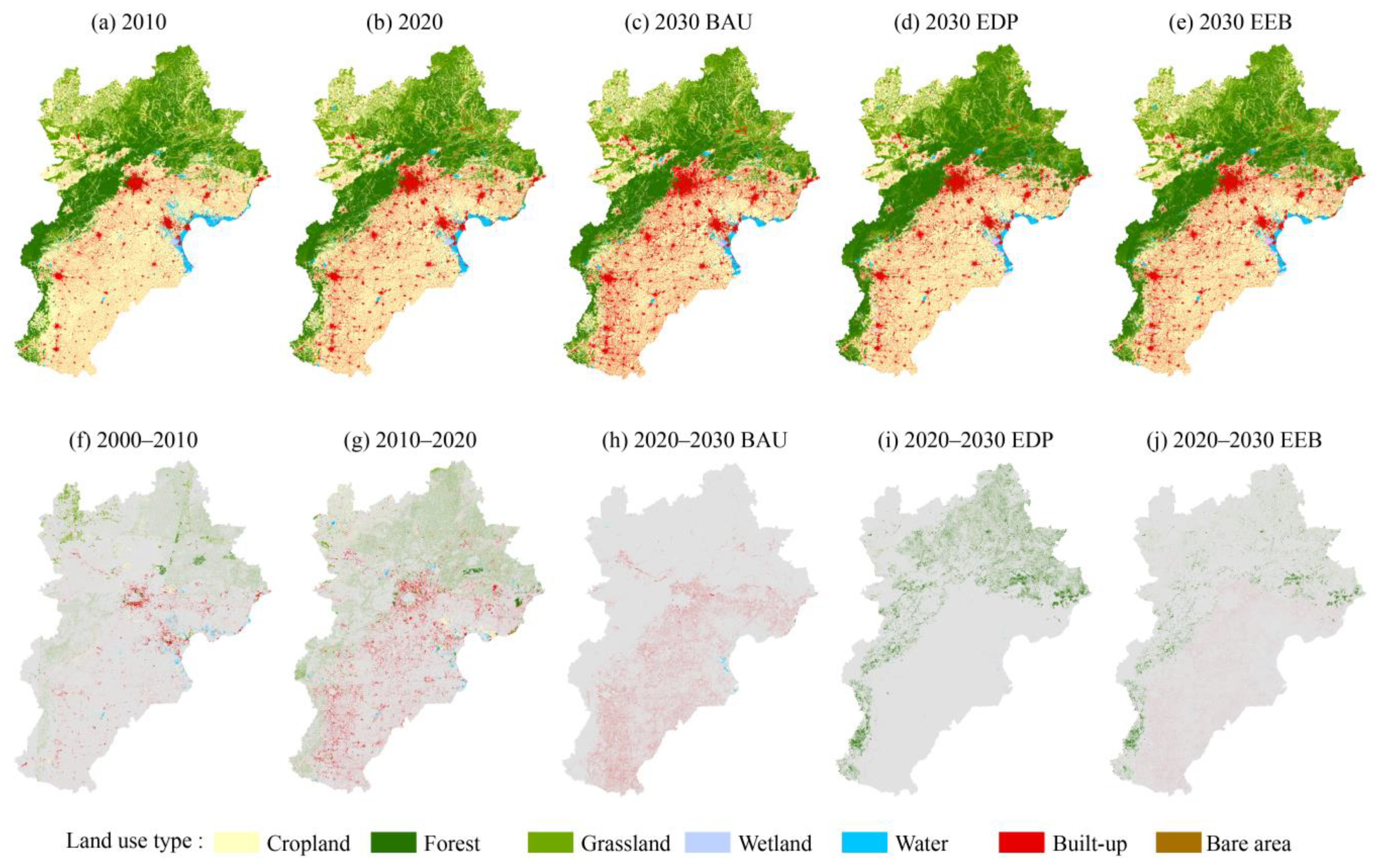
According to Figure 5a,b,f,g, the transition between cropland, woodland, and grassland, best reflects the historical evolution. A lot of croplands were being invaded by the rapid rise of the built-up area. As shown in

Table 3. Area changes of historical and simulation LULC.

Land Use Types	Cropland	Forest	Grassland	Wetland	Water	Built-Up	Bare Land
2000	116,307.69	41,704.91	37,877.92	663.81	3970.40	14,920.37	71.26
2010	112,590.41	42,053.62	38,566.72	843.55	3785.50	17,655.77	74.22
2020	104,477.76	42,173.93	38,126.48	603.85	3762.59	26,207.06	232.3
BAU	97,972.17	42,153.18	37,656.82	444.7	3497.71	32,973.74	187.17
EDP	95,219.96	53,542.90	35,770.75	671.81	3463.27	26,072.76	144.04
EEB	96,704.18	46,130.64	39,542.89	671.75	3463.27	28,183.91	188.85

, the following were the primary LULC changes during this time: (1) There was a trend toward less cropland and water. 11,829.93 km² cropland decreased, of which 66.38 % was converted to built-up, which was then replaced by grassland (21.26%). A total of 207.81 km² of water were lost, primarily due to agricultural and built-up areas (80.20%). (2) The amount of forest, built-up, and bare land, showed an upward tendency. Cropland and grassland provided 99.06% of the growth in forest, which increased by 469.02 km². The built-up area had increased by 75% to around 26,207.06 km² in 2020 compared to 2010, and the growth rate was still increasing. The loss of grassland was primarily responsible for the expansion of bare land. (3) An inverted “U”-shaped trend of growing and then dropping in both grassland and wetland. The grassland area increased by 0.62% and was largely constant. Wetland area declined by 9.06%, primarily due to a shift to cropland and water. (4) There were obvious spatial variations in the changes of the various land types. As seen in Figure 5f,g, the Taihang Mountains to the north and west of the study area were the primary locations for the spread of grassland and forest. The North China Plain study area’s central and eastern regions had the greatest growth in built-up, with the pattern of growth showing a spread outward from the urban core. Both the water conservation area and the eastern Bohai Sea coastline zone were affected by the growth of water. These results were in line with earlier research on the mechanisms affecting land use expansion, and they once more demonstrate how topography, hydrothermal conditions, and economic status, can all have an impact on LULC change.

The LULC simulation results of the three scenarios in 2030 are shown in Figure 5c–e. They demonstrated that the differences in simulation outcomes clearly had an impact on goals. Under BAU scenario (Figure 5c,h), the growth of forest and grassland in the mountainous areas of the western part of the study area was at a standstill. Built-up in the central and southern plains of the study area expanded significantly, with a growth rate of 25.83%. The wetland area showed a decreasing trend (at 26.36%), mainly transformed into forest and water. Social construction under the BAU scenario would continue the trend of 2000–2020, with a policy focus favoring socioeconomic development. The socio-economic benefits of LULC increased by about 22.08% and the ESV decreased by about 3.13%. Under the EDP scenario (Figure 5d,i), the growth of built-up was at a stagnant state compared to 2020. The area of forest and wetland increased by 26.96% and 11.25%, with 37.99% reduction in bare land. Cropland, water, and grassland, decreased by 8.86%, 7.96%, and 6.18%, respectively. These changes resulted in a 5.52% increase in ESV and a 1.08% decrease in economic benefits in the study area under the EDP scenario. Under the EEB scenario, the three types of ecological land (i.e., forest, grassland, and wetland) showed an increasing trend with a slowdown in the growth of built-up land (Figure 5e,j). Cropland and water showed a decreasing trend, and the area of bare land remains stable. Compared to 2020, the ESV increased by 1.69% and the socio-economic benefits increased by 6.40%. In summary, the degree of LULC change under the EEB scenario was between the BAU scenario and the EDP scenario, so the development objectives of the EEB scenario better reflected the balance between ESV and socio-economic benefits.

4.2. Dynamic Simulation of CS at Patch Scale

The aboveground, belowground biomass, and topsoil organic carbon densities of different land use types were calculated using overlay analysis based on the LULC data and carbon density data, (

Table 4. Average carbon density for each land use type (Mg/km²).

Land Use Types	Cropland	Forest	Grassland	Wetland	Water	Built-Up	Bare Land
Aboveground carbon density	2348.01	9983.16	4622.73	1311.80	783.92	1370.08	4035.54
Belowground carbon density	1462.40	6885.94	4867.36	3140.96	967.33	2238.91	4036.65
Topsoil organic carbon density	3948.14	5739.06	4909.30	4181.36	3897.12	3803.45	5227.20

).

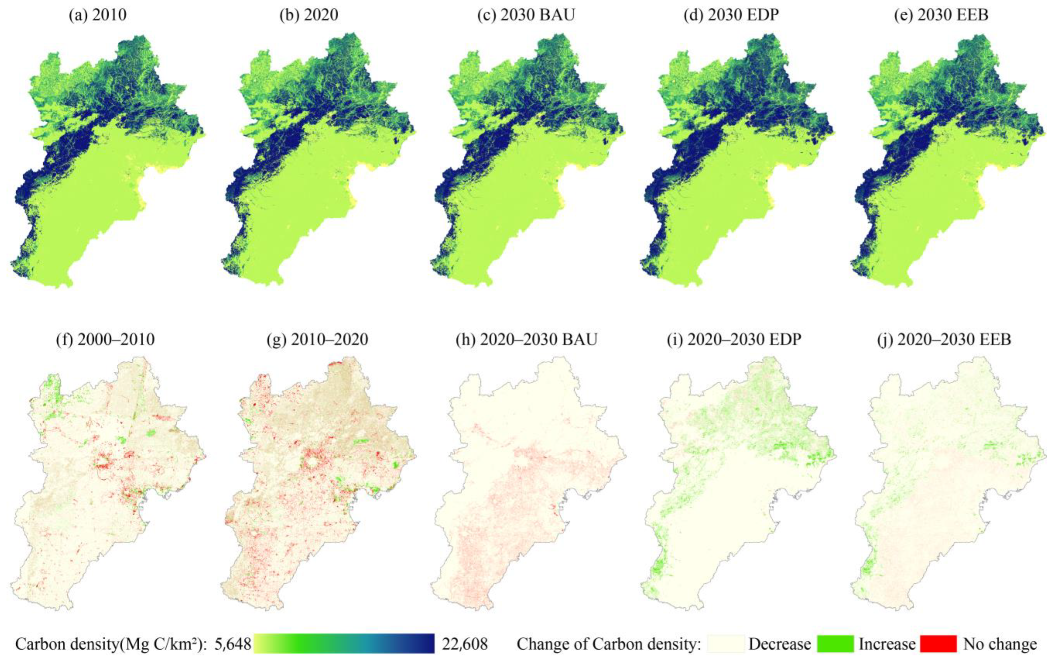
To explore the characteristics of CS under the three scenarios, the historical and future simulation LULC results were input into InVEST, as shown in Figure 6. The carbon storage was characterized by “high in the northwest and low in the southeast”, and the maximum and minimum values of carbon storage are 22,608 Mg/km² and 5648 Mg/km², respectively. As shown in

Table 5. Carbon storage history and multi-scenario estimation results (Tg).

CS (Tg)	Cropland	Forest	Grassland	Wetland	Water	Built-Up	Bare Area	Total
2000	902.38	942.87	545.42	5.73	22.43	110.60	0.95	2530.37
2010	873.54	950.76	555.34	7.28	21.38	130.87	0.99	2540.16
2020	810.60	953.48	549.00	5.21	21.25	194.26	3.09	2536.88
BAU	760.12	953.01	542.24	3.84	19.76	244.42	2.49	2525.86
EDP	738.77	1210.51	515.08	5.80	19.56	193.26	1.92	2684.89
EEB	750.28	1042.93	569.39	5.80	19.56	208.91	2.51	2599.39
2000–2010	−28.84	7.88	9.92	1.55	−1.04	20.28	0.04	9.78
2010–2020	−62.94	2.72	−6.34	−2.07	−0.13	63.39	2.10	−3.27
BAU	−50.47	−0.47	−6.76	−1.37	−1.50	50.16	−0.60	−11.02
EDP	−71.83	257.03	−33.92	0.59	−1.69	−1.00	−1.17	148.01
EEB	−60.31	89.45	20.40	0.59	−1.69	14.65	−0.58	62.51

, forest, cropland, and grassland, contributed the most to the carbon storage. Through Figure 6f,g, the expansion of build-up in the plains and the encroachment of forest in higher elevations lead to a general decreasing trend of CS in the study area. Compared with 2000–2010, the area of CS decline increased and the degree of decline deepened from 2010–2020. From 2000 to 2010, CS in the study area increased by 9.78 Tg, mainly in the “Northern Sand Control Zone” in the northwestern part, showing a connected aggregation. During 2010–2020, the CS in the study area decreased by 3.27 Tg, and the carbon sink capacity only part of the “Water Containment Ecological Function Reserve” showed an increasing trend.

For the three scenarios, the spatial pattern of CS in 2030 was the same as that in 2010–2020. The increase in CS was most significant in the northwestern part of the study area under the EDP scenario, followed by the EEB scenario, while the change was not obvious under the BAU scenario. Under the BAU scenario, CS in most areas of the study area showed a decreasing trend, with the most significant decrease in the North China Plain, and the CS increase area was mainly located in the Bohai Sea coastal zone (Figure 6c,h). Under the EDP scenario, the expansion of forest in the northwest and wetlands in the northeast led to the increase of regional carbon stock at 148.01 Tg, while the change in CS in the North China Plain was smaller (Figure 6d,i). The variation of CS in EEB scenario was between EDP and BAU scenarios. As shown in Table 5, the study area had the highest CS at 2684.89 Tg under EDP scenario, which is an increase of 5.83% (148.01 Tg) compared to 2020. Under EEB scenario, future CS was 2599.39 Tg, which is an increase of 2.46% compared to 2020. The CS was the least in BAU scenario (2525.86 Tg), which is a decrease of 0.43% (11.02 Tg).

4.3. Evolution Prospect of CS at Regional Scale

The results in the previous Section 4.2 shows the distribution pattern and evolutionary characteristics of CS at the patch scale. To further explore the CS variation at the regional scale, the CS of 13 cities in the study area were counted with the help of geographic information technology, as shown in

Table 6. CS change at the city-level scale.

	CS/Tg					Change of CS/Tg
	2010	2020	BAU	EDP	EEB	2000–2010	2010–2020	BAU	EDP	EEB
Beijing	243.79	244.38	243.12	252.66	247.96	0.06	0.59	−1.08	8.46	3.76
Tianjin	91.10	91.78	90.53	91.94	91.25	−0.19	0.67	−0.45	0.96	0.27
Shijiazhuang	159.69	158.75	158.35	168.32	165.55	−0.18	−0.94	−0.35	9.62	6.85
Tangshan	116.97	117.76	115.02	125.50	120.53	0.49	0.77	−0.71	9.77	4.81
Qinhuangdao	96.58	99.98	98.83	115.52	107.06	0.06	3.39	−0.26	16.44	7.98
Handan	112.83	112.61	112.13	117.34	114.95	−0.23	−0.22	−0.33	4.87	2.49
Xingtai	110.55	110.18	109.87	120.02	117.70	−0.04	−0.37	−0.28	9.87	7.55
Baoding	290.17	288.35	288.00	302.45	298.21	−0.09	−1.82	−0.32	14.14	9.90
Zhangjiakou	465.05	459.32	458.63	481.57	467.82	8.70	−5.73	−0.59	22.35	8.60
Chengde	620.06	620.92	620.40	677.42	636.50	1.27	0.86	−0.41	56.62	15.70
Cangzhou	107.33	106.94	106.11	106.47	106.39	−0.07	−0.39	−0.35	0.01	−0.07
Langfang	49.51	49.59	49.24	49.67	49.60	−0.44	0.08	−0.34	0.09	0.02
Hengshui	68.04	67.87	67.67	67.85	67.79	−0.10	−0.17	−0.19	−0.01	−0.07

. Combined with the spatial distribution of CS changes under different time periods and scenarios (Figure 6), the 13 cities showed significant spatial heterogeneity. In terms of spatial location from 2000 to 2010, CS in the northern part of the study area showed a decreasing trend, and in the central and southern parts of the study area showed an increasing trend. From 2010 to 2020, CS in the northeast of the study area showed an increasing trend, while the CS in the southwest showed a decreasing trend. For each city, Chengde had the highest CS in 2010 and 2020, with 620.06 Tg and 620.92 Tg, respectively. In 2010 and 2020, both Baoding and Beijing hold CS greater than 200 Tg, Shijiazhuang, Tangshan, Handan, Xingtai, and Cangzhou, were larger than 100 Tg, and Langfang had the smallest CS at less than 50 Tg. From 2000 to 2010, the CS in Zhangjiakou and Chengde showed a significant increasing trend, with an amount of 8.70 Tg and 1.27 Tg, respectively. The CS in Handan and Tangshan showed a minor decrease trend, by 0.23 Tg and 0.19 Tg, respectively. From 2010 to 2020, the CS in Qinhuangdao, Chengde, Tangshan, Tianjin, and Beijing, showed a clear increasing trend, with an increase of 3.39 Tg, 0.86 Tg, 0.77 Tg, 0.67 Tg, and 0.59 Tg, respectively. The CS in Zhangjiakou, Baoding and Shijiazhuang showed a clear trend of decrease, by 5.73 Tg, 1.82 Tg, and 0.94 Tg, respectively.

The results also showed that the changes of CS under the three scenarios have significant differences, both the northern and western parts of the study area showed an increasing trend in CS, while the central and southern parts showed a decreasing trend in CS. Under BAU scenario, the CS of all 13 cities showed a decreasing trend, with the most obvious decrease in Beijing (1.08 Tg). Under EDP scenario, the CS of all 13 cities showed an increasing tendency, with the increase of CS in Chengde, Zhangjiakou, Qinhuangdao, and Baoding, being greater than 10 Tg. Under EEB scenario, the CS of four cities (i.e., Tianjin, Langfang, Cangzhou, and Hengshui) were relatively stable, while the CS of the remaining cities show an increasing trend, with the most significant increase (15.70 Tg) in Chengde. Therefore, the carbon sink function in Hengshui and Cangzhou faces certain risks in the future.

5. Discussion

5.1. MPI Coupling Model

Simulating LULC and CS dynamics is critical for rational land use planning under the background of China’s quest of “carbon neutrality” [55]. Some researchers have pointed out that the traditional estimating models of CS have the disadvantages of extensive parameter setting and difficult operation, so the simulation models of LULC have the shortcomings of low accuracy, poor disclosure, and poor applicability [21]. To overcome the above problems, this work suggested a MOP-PLUS-InVEST coupling model (named MPI) that fully exploits the benefits of each of them. The MOP model is a quantitative optimization model for LULC that can determine demand for each land use type according to the study area’s historical land use evolution characteristics and current territorial spatial planning policies. The PLUS model then simulates the spatial distribution of LULC based on the demand and growth probability of each land type, and during this process, spatial restrictions can be imposed on multiple regions and land use types as needed to meet the specific needs of ecological restoration, arable land conservation, and so on. Finally, by integrating the LULC simulation results into the InVEST model for investigating CS changes at several scales, the results of the spatial and temporal evolution of CS are swiftly produced. The MPI model thus aids in the formulation and adjustment of land use planning. Furthermore, the results of the MPI model can be integrated with the results of other models to broaden its applications, such as biodiversity and soil conservation [56], calculating ESV [57], and performing landscape pattern analysis [58].

5.2. Evolution of LULC and CS

LULC changes have a major impact on the carbon sink function of terrestrial ecosystems [33,34]. Rapid urbanization and economic development have resulted in a decrease in CS in major portions of China. This research is to determine whether a “win-win” situation of ecological function and economic value can be achieved through a reasonable LULC spatial distribution. Under the BAU scenario, ESV decreased by 3.13% and economic benefit increased by 22.8%, and under the EDP scenario, ESV increased by 5.52% and economic benefit decreased by 1.08%. However, under the EDP scenario, ESV and EC increased by 1.69% and 6.40%, respectively. The result proved that the EEB scenario, which weighs economy and ecology, is a reference for BTH to achieve a coordinated and sustainable development approach. This is also consistent with a number of related studies, such as Li et al.’s study on the ecological barrier zone in Sichuan-Yunnan, China, which noted that a feasible scenario to a green economy involves balancing the ecological carrying capacity and the spatial arrangement of economic construction [35].

LULC changes in BTH are still dominated by the mutual transfer of cropland, forest, and grassland, while the implementation of the “Grain for Green Project” has obviously accelerated the transfer of cropland out to another two types. The increase in the total area of four categories of ecological land: water bodies, wetlands, woodlands, and grasslands, is the result of the implementation of ecological conservation policies in BTH [36]. Water is an important part of the ecological land use, and continuous water systems play a vital role in the improvement of the neighborhood environment and the full play of ecological services, but the area of water bodies in BTH still shows a trend of shrinking, and water pollution and water degradation are still urgent issues that need to be resolved.

Currently, the CS in BTH is about 2536.88 Tg, of which the aboveground biomass, belowground biomass, and topsoil organic carbon pool, account for 34.81%, 27.35, and 37.83%, respectively. It is expected that the CS in BTH will be 2525.86–2684.89 Tg in 2030. Cropland and forests, which together make up 37.58% and 31.95% CS, are the most significant land use types. Vegetation’s ability to act as a carbon sink is influenced by its phenology. Between 2000 and 2020, new forests were created on 1247.51 km² of cropland and 5912.63 km² of grassland, but the CS in northwest BTH expanded slowly since it was at the early age. The capacity of plants to absorb carbon increases with size, and as the forest in the BTH will continue to grow in all three scenarios, it has the potential to be a very significant carbon sink.

5.3. Potential Ecological Threat

As mentioned above, the interconversion of cropland, grassland, and forest, accounts for the majority of the carbon gains in BTH. However, local governments must also be aware of the potential ecological risks posed by such phenomena. Water performs significant roles, even though it contributes less to CS than other land use types [17]. However, due to the current protection laws not being perfect, water bodies in BTH are at considerable risk of degrading. Forest ecological processes are significantly impacted by deforestation and fires, hence stringent conservation of forests must persist. On the other hand, investigating ecological changes at various scales and levels is a crucial step in developing a future plan for ecological issues. Because different sizes and different research subjects will lead to variances in outcomes, Liang et al.’s simulation analysis of China’s CS demonstrates that the future CS in BTH tends to decline [21]. As a result, a multi-scale investigation was carried out in this study, and the findings indicate that the carbon sink functions of Hengshui and Cangzhou cities in the southeast of BTH are in jeopardy and require policymakers’ attention. Moreover, according to the outcome envisaged by the EEB scenario, the restoration of ecological functions and economic development are not completely contradictory, so ecological protection cannot be implemented in an all-encompassing way.

5.4. Limitations and Prospects

A new approach suitable for exploring the simulation of LULC and CS evolution at the regional scale was proposed in this research, but there are still some points that need to improve. First, the MOP model’s practical application is easily constrained by the level of detail of relevant data in the study region because it is a highly targeted LULC structure optimization method. Similar research has been cited in this paper to strengthen the LULC limitations in addition to closely adhering to the land use planning of BTH. Second, the partial lack of the LULC data and driving variables will result in missing pixels on the result images, which inherently affects the results’ correctness. Third, there are still some uncertainties in the CS estimation results. Although mature carbon density data were used, the results are uncertain because the InVEST model ignores variations in carbon density within different land use types. This is because carbon density is likely to undergo subtle dynamic changes over time due to the human activities and environmental changes.

Future studies should concentrate on: (1) integrating various techniques to look at more standardized and effective ways to improve LULC structure; (2) examining ways to build dynamic systems of land use and carbon density drivers, taking into account the dynamic effects of human activity and natural environmental changes on the ecosystems’ capacity to store carbon; and (3) making empirical measurements to examine the variation within different land use types and validating model findings with adequate empirical data to raise the precision of regional terrestrial ecosystem CS evaluations.

6. Conclusions

In rapidly urbanizing regions, economic development and anthropogenic disturbances have resulted in substantial LULC, which has a significant impact on ecosystem functions and services. It is critical to assess the spatiotemporal evolution of LULC and terrestrial ecosystem CS in these areas, especially for the BTH in China.

In this study, a MOP-PLUS-InVEST coupling model was proposed to simulate the LULC and CS in 2030 in the BTH, based on the historical trends from 2000 to 2020. The evolution of LULC in BTH were mostly represented in transfers between cropland, forest, and grassland. The historical changes were characterized by the reduction of cropland and water, and the increase of forest, built-up and bare land, among which 11,286.7 km² of built-up land occupied a large amount of ecological land. The BAU scenario demonstrated the most dramatic increase in built-up, with small changes in forest and grassland, and hence the economic benefits rose. In the EDP scenario, forest and wetland developed dramatically, while built-up remained stagnant, restoring the ecological function. In the EEB scenario, ecological land increased while built-up expanded slowly, resulting in economic and ecological benefits. The constant shrinking of water is a pressing issue that must be addressed in the future. In terms of CS evolution, among the various land use types, forest, cropland, and grassland, contributed the most of the carbon storage. Influenced by land use distribution and topography, the distribution of CS was high in the northwest and low in the southeast. At the same time, the change of CS was affected by the construction of ecological conservation area and urban construction, showed obvious spatial differences. The 2020 CS of BTH was 2536.88 Tg, and the predicted results under BAU, EDP, and EEB scenarios were 2525.86 Tg, 2684.89 Tg, and 2599.39 Tg, respectively, with CS increasing mostly in the western and northern regions. The EEB scenario balanced ecological services and economic rewards, increased the ecosystem carbon sink function, and is an efficient way to investigate “carbon neutrality”.

References

1. Boot-Handford, M.E.; Abanades, J.C.; Anthony, E.J.; Blunt, M.J.; Brandani, S.; Mac Dowell, N.; Fernandez, J.R.; Ferrari, M.-C.; Gross, R.; Hallett, J.P.; et al. Carbon capture and storage update. Energy Environ. Sci. 2014, 7, 130–189. [Google Scholar] [CrossRef]
2. Snaebjornsdottir, S.O.; Sigfusson, B.; Marieni, C.; Goldberg, D.; Gislason, S.R.; Oelkers, E.H. Carbon dioxide storage through mineral carbonation. Nat. Rev. Earth Environ. 2020, 1, 90–102. [Google Scholar] [CrossRef] [Green Version]
3. Wang, X.; Feng, Z.; Ouyang, Z. Vegetation carbon storage and density of forest ecosystems in China. Chin. J. Appl. 2001, 12, 13–16. [Google Scholar] [CrossRef]
4. Garcia, R.A.; Cabeza, M.; Rahbek, C.; Araújo, M.B. Multiple Dimensions of Climate Change and Their Implications for Biodiversity. Science 2014, 344, 1247579. [Google Scholar] [CrossRef] [Green Version]
5. Wheeler, T.; von Braun, J. Climate Change Impacts on Global Food Security. Science 2013, 341, 508–513. [Google Scholar] [CrossRef]
6. Ma, Z.; Liu, H.; Mi, Z.; Zhang, Z.; Wang, Y.; Xu, W.; Jiang, L.; He, J.-S. Climate warming reduces the temporal stability of plant community biomass production. Nat. Commun. 2017, 8, 15378. [Google Scholar] [CrossRef] [Green Version]
7. Liu, Y.Y.; van Dijk, A.I.J.M.; de Jeu, R.A.M.; Canadell, J.G.; McCabe, M.F.; Evans, J.P.; Wang, G. Recent reversal in loss of global terrestrial biomass. Nat. Clim. Chang. 2015, 5, 470–474. [Google Scholar] [CrossRef]
8. Chen, S.; Wang, W.; Xu, W.; Wang, Y.; Wan, H.; Chen, D.; Tang, Z.; Tang, X.; Zhou, G.; Xie, Z.; et al. Plant diversity enhances productivity and soil carbon storage. Proc. Natl. Acad. Sci. USA 2018, 115, 4027–4032. [Google Scholar] [CrossRef] [Green Version]
9. Sohl, T.L.; Sleeter, B.M.; Zhu, Z.; Sayler, K.L.; Bennett, S.; Bouchard, M.; Reker, R.; Hawbaker, T.; Wein, A.; Liu, S.; et al. A land-use and land-cover modeling strategy to support a national assessment of carbon stocks and fluxes. Appl. Geogr. 2012, 34, 111–124. [Google Scholar] [CrossRef]
10. Ghafoor, G.Z.; Sharif, F.; Shahid, M.G.; Shahzad, L.; Rasheed, R.; Khan, A.U.H. Assessing the impact of land use land cover change on regulatory ecosystem services of subtropical scrub forest, Soan Valley Pakistan. Sci. Rep. 2022, 12, 10052. [Google Scholar] [CrossRef]
11. Xie, X.; Sun, B.; Zhou, H.; Li, P.; Li, A. Organic carbon density and storage in soils of China and spatial analysis. Acta Pedol. Sin. 2004, 41, 35–43. [Google Scholar] [CrossRef]
12. Friedlingstein, P.; O’Sullivan, M.; Jones, M.W.; Andrew, R.M.; Hauck, J.; Olsen, A.; Peters, G.P.; Peters, W.; Pongratz, J.; Sitch, S.; et al. Global Carbon Budget 2020. Earth Syst. Sci. Data 2020, 12, 3269–3340. [Google Scholar] [CrossRef]
13. Mallapaty, S. How China Could Be Carbon Neutral by Mid-Century. Nature 2020, 586, 482–483. [Google Scholar] [CrossRef]
14. Zhao, X.; Ma, X.; Chen, B.; Shang, Y.; Song, M. Challenges toward carbon neutrality in China: Strategies and countermeasures. Resour. Conserv. Recycl. 2022, 176, 105959. [Google Scholar] [CrossRef]
15. Mirici, M.E.; Berberoglu, S.; Akin, A.; Satir, O. Land Use/Cover Change Modelling in a Mediterranean Rural Landscape Using Multi-Layer Perceptron and Markov Chain (mlp-Mc). Appl. Ecol. Environ. Res. 2018, 16, 467–486. [Google Scholar] [CrossRef]
16. Guo, Z.; Hu, H.; Li, P.; Li, N.; Fang, J. Spatio-temporal changes in biomass carbon sinks in China’s forests from 1977 to 2008. Sci. China Life Sci. 2013, 56, 661–671. [Google Scholar] [CrossRef] [Green Version]
17. Wang, X.; Li, R.; Ding, H.; Fu, Y. Fine-Scale Improved Carbon Bookkeeping Model Using Landsat Time Series for Subtropical Forest, Southern China. Remote Sens. 2022, 14, 753. [Google Scholar] [CrossRef]
18. Tang, X.; Zhao, X.; Bai, Y.; Tang, Z.; Wang, W.; Zhao, Y.; Wan, H.; Xie, Z.; Shi, X.; Wu, B.; et al. Carbon pools in China’s terrestrial ecosystems: New estimates based on an intensive field survey. Proc. Natl. Acad. Sci. USA 2018, 115, 4021–4026. [Google Scholar] [CrossRef] [Green Version]
19. Du, H.; Mao, F.; Zhou, G.; Li, X.; Xu, X.; Ge, H.; Cui, L.; Liu, Y.; Zhu, D.; Li, Y. Estimating and Analyzing the Spatiotemporal Pattern of Aboveground Carbon in Bamboo Forest by Combining Remote Sensing Data and Improved BIOME-BGC Model. IEEE J. Sel. Top. Appl. Earth Obs. Remote Sens. 2018, 11, 2282–2295. [Google Scholar] [CrossRef]
20. Zhang, L.; Zhou, G.; Ji, Y.; Bai, Y. Spatiotemporal dynamic simulation of grassland carbon storage in China. Sci. China-Earth Sci. 2016, 59, 1946–1958. [Google Scholar] [CrossRef]
21. Liu, X.; Li, X.; Liang, X.; Shi, H.; Ou, J. Simulating the Change of Terrestrial Carbon Storage in China Based on the FLUS-InVEST Model. Tropicalgeography 2019, 39, 397–409. [Google Scholar] [CrossRef]
22. González-García, A.; Palomo, I.; González, J.A.; López, C.A.; Montes, C. Quantifying spatial supply-demand mismatches in ecosystem services provides insights for land-use planning. Land Use Policy 2020, 94, 104493. [Google Scholar] [CrossRef]
23. Li, X.; Huang, C.; Jin, H.; Han, Y.; Kang, S.; Liu, J.; Cai, H.; Hu, T.; Yang, G.; Yu, H.; et al. Spatio-Temporal Patterns of Carbon Storage Derived Using the InVEST Model in Heilongjiang Province, Northeast China. Front. Earth Sci. 2022, 10, 846456. [Google Scholar] [CrossRef]
24. Adelisardou, F.; Zhao, W.; Chow, R.; Mederly, P.; Minkina, T.; Schou, J.S. Spatiotemporal change detection of carbon storage and sequestration in an arid ecosystem by integrating Google Earth Engine and InVEST (the Jiroft plain, Iran). Int. J. Environ. Sci. Technol. 2021, 19, 5929–5944. [Google Scholar] [CrossRef]
25. Zhao, L.; Yang, J.; Li, C.; Ge, Y.; Han, Z. Progress on Geographic Cellular Automata Model. Sci. Geogr. Sin. 2016, 36, 1190–1196. [Google Scholar] [CrossRef]
26. Wang, Z.; Li, X.; Mao, Y.; Li, L.; Wang, X.; Lin, Q. Dynamic simulation of land use change and assessment of carbon storage based on climate change scenarios at the city level: A case study of Bortala, China. Ecol. Indic. 2022, 134, 108499. [Google Scholar] [CrossRef]
27. Li, X.; Yeh, A.G. Neural-network-based cellular automata for simulating multiple land use changes using GIS. Int. J. Geogr. Inf. Sci. 2002, 16, 323–343. [Google Scholar] [CrossRef]
28. Verburg, P.H.; Soepboer, W.; Veldkamp, A.; Limpiada, R.; Espaldon, V.; Mastura, S.S.A. Modeling the spatial dynamics of regional land use: The CLUE-S model. Environ. Manag. 2002, 30, 391–405. [Google Scholar] [CrossRef]
29. Liu, X.; Liang, X.; Li, X.; Xu, X.; Ou, J.; Chen, Y.; Li, S.; Wang, S.; Pei, F. A future land use simulation model (FLUS) for simulating multiple land use scenarios by coupling human and natural effects. Landsc. Urban Plan. 2017, 168, 94–116. [Google Scholar] [CrossRef]
30. Liang, X.; Guan, Q.; Clarke, K.C.; Liu, S.; Wang, B.; Yao, Y. Understanding the drivers of sustainable land expansion using a patch-generating land use simulation (PLUS) model: A case study in Wuhan, China. Comput. Environ. Urban Syst. 2021, 85, 101569. [Google Scholar] [CrossRef]
31. Zhu, W.; Zhang, J.; Cui, Y.; Zheng, H.; Zhu, L. Assessment of territorial ecosystem carbon storage based on land use change scenario: A case study in Qihe River Basin. Acta Geogr. Sin. 2019, 74, 446–459. [Google Scholar] [CrossRef]
32. Yao, Y.; Liu, X.; Li, X.; Liu, P.; Hong, Y.; Zhang, Y.; Mai, K. Simulating urban land-use changes at a large scale by integrating dynamic land parcel subdivision and vector-based cellular automata. Int. J. Geogr. Inf. Sci. 2017, 31, 2452–2479. [Google Scholar] [CrossRef]
33. Guan, D.; Zhao, Z.; Tan, J. Dynamic simulation of land use change based on logistic-CA-Markov and WLC-CA-Markov models: A case study in three gorges reservoir area of Chongqing, China. Environ. Sci. Pollut. Res. 2019, 26, 20669–20688. [Google Scholar] [CrossRef] [PubMed]
34. Wang, Y.; Li, X.; Zhang, Q.; Li, J.; Zhou, X. Projections of future land use changes: Multiple scenarios-based impacts analysis on ecosystem services for Wuhan city, China. Ecol. Indic. 2018, 94, 430–445. [Google Scholar] [CrossRef]
35. Li, C.; Wu, Y.; Gao, B.; Zheng, K.; Wu, Y.; Li, C. Multi-scenario simulation of ecosystem service value for optimization of land use in the Sichuan-Yunnan ecological barrier, China. Ecol. Indic. 2021, 132, 108328. [Google Scholar] [CrossRef]
36. Yang, Y.; Bao, W.; Liu, Y. Scenario simulation of land system change in the Beijing-Tianjin-Hebei region. Land Use Policy 2020, 96, 104677. [Google Scholar] [CrossRef]
37. Wu, A.; Zhang, J.; Zhao, Y.; Shen, H.; Guo, X. Simulation and Optimization of Supply and Demand Pattern of Multiobjective Ecosystem Services—A Case Study of the Beijing-Tianjin-Hebei Region. Sustainability 2022, 14, 2658. [Google Scholar] [CrossRef]
38. Wu, J.; Jin, X.; Feng, Z.; Chen, T.; Wang, C.; Feng, D.; Lv, J. Relationship of Ecosystem Services in the Beijing–Tianjin–Hebei Region Based on the Production Possibility Frontier. Land 2021, 10, 881. [Google Scholar] [CrossRef]
39. Zhang, D.; Huang, Q.; He, C.; Wu, J. Impacts of urban expansion on ecosystem services in the Beijing-Tianjin-Hebei urban agglomeration, China: A scenario analysis based on the Shared Socioeconomic Pathways. Resour. Conserv. Recycl. 2017, 125, 115–130. [Google Scholar] [CrossRef]
40. Lv, J.; Wang, Y.; Liang, X.; Yao, Y.; Ma, T.; Guan, Q. Simulating urban expansion by incorporating an integrated gravitational field model into a demand-driven random forest-cellular automata model. Cities 2021, 109, 103044. [Google Scholar] [CrossRef]
41. Jun, C.; Ban, Y.; Li, S. Open access to Earth land-cover map. Nature 2014, 514, 434. [Google Scholar] [CrossRef] [PubMed] [Green Version]
42. Spawn, S.A.; Sullivan, C.C.; Lark, T.J.; Gibbs, H.K. Harmonized global maps of above and belowground biomass carbon density in the year 2010. Sci. Data 2020, 7, 112. [Google Scholar] [CrossRef] [Green Version]
43. Food and Agriculture Organization of the United Nations. Global Soil Organic Carbon Sequestration Potential Map (GSOCseq v1.1) Technical Report; FAO: Rome, Italy, 2022. [Google Scholar]
44. Xie, G.; Zhang, C.; Zhang, C.; Xiao, Y.; Lu, C. The value of ecosystem services in China. Resour. Sci. 2015, 37, 1740–1746. [Google Scholar]
45. Yanfang, L.; Dongping, M.; Jianyu, Y. Optimization of land use structure based on ecological GREEN equivalent. Geo-Spat. Inf. Sci. 2002, 5, 60–67. [Google Scholar] [CrossRef]
46. Xin, L.; Wang, J.; Wang, L. Prospect of per capita grain demand driven by dietary structure change in China. Resour. Sci. 2015, 37, 1347–1356. [Google Scholar]
47. Li, Z.; Liu, S.; Sun, R.; Sun, W. Identifying the temporal-spatial pattern evolution of the multiple cropping index in the Huang-Huai-Hai region. Acta Ecol. Sin. 2018, 38, 4454–4460. [Google Scholar] [CrossRef]
48. Yu, L.; Gu, F.; Huang, M.; Tao, B.; Hao, M.; Wang, Z. Impacts of 1.5 °C and 2 °C Global Warming on Net Primary Productivity and Carbon Balance in China’s Terrestrial Ecosystems. Sustainability 2020, 12, 2849. [Google Scholar] [CrossRef] [Green Version]
49. Zhai, H.; Lv, C.; Liu, W.; Yang, C.; Fan, D.; Wang, Z.; Guan, Q. Understanding Spatio-Temporal Patterns of Land Use/Land Cover Change under Urbanization in Wuhan, China, 2000–2019. Remote Sens. 2021, 13, 3331. [Google Scholar] [CrossRef]
50. Adedeji, O.H.; Elegbede, I.O. Chapter 12—Mapping and Modeling Ecosystem Services in Petroleum-Producing Areas in Nigeria. In The Political Ecology of Oil and Gas Activities in the Nigerian Aquatic Ecosystem; Ndimele, P.E., Ed.; Academic Press: Cambridge, MA, USA, 2018; pp. 159–175. ISBN 978-0-12-809399-3. [Google Scholar]
51. Shah, M.A.R.; Renaud, F.G.; Anderson, C.C.; Wild, A.; Domeneghetti, A.; Polderman, A.; Votsis, A.; Pulvirenti, B.; Basu, B.; Thomson, C.; et al. A review of hydro-meteorological hazard, vulnerability, and risk assessment frameworks and indicators in the context of nature-based solutions. Int. J. Disaster Risk Reduct. 2020, 50, 101728. [Google Scholar] [CrossRef]
52. Tang, L.; Ke, X.; Zhou, T.; Zheng, W.; Wang, L. Impacts of cropland expansion on carbon storage: A case study in Hubei, China. J. Environ. Manag. 2020, 265, 110515. [Google Scholar] [CrossRef]
53. Dang, A.N.; Jackson, B.M.; Benavidez, R.; Tomscha, S.A. Review of ecosystem service assessments: Pathways for policy integration in Southeast Asia. Ecosyst. Serv. 2021, 49, 101266. [Google Scholar] [CrossRef]
54. Taffarello, D.; Calijuri, M.D.C.; Viani, R.A.G.; Marengo, J.A.; Mendiondo, E.M. Hydrological services in the Atlantic Forest, Brazil: An ecosystem-based adaptation using ecohydrological monitoring. Clim. Serv. 2017, 8, 1–16. [Google Scholar] [CrossRef]
55. Ma, T.; Li, X.; Bai, J.; Ding, S.; Zhou, F.; Cui, B. Four decades’ dynamics of coastal blue carbon storage driven by land use/land cover transformation under natural and anthropogenic processes in the Yellow River Delta, China. Sci. Total Environ. 2019, 655, 741–750. [Google Scholar] [CrossRef] [PubMed]
56. Pan, M.; Zhang, L.; Hu, T.; Hao, Y. Temporal and spatial changes and trade-offs analysis of urban wetland ecosystem services: A case study of Xixi wetland in Hangzhou. J. Beijing Norm. Univ. 2022, 2022, 1–9. [Google Scholar] [CrossRef]
57. Xu, Y.; Xiao, F. Assessing Changes in the Value of Forest Ecosystem Services in Response to Climate Change in China. Sustainability 2022, 14, 4773. [Google Scholar] [CrossRef]
58. Teng, Y.; Yan, Y.; Guo, W.; Li, K.; Zhao, C. Analysis of Spatiao-temporal Variation of Ecological Environment in Mining City Based on Remote Sensing Ecology Index. Met. Mine 2022, 2022, 1–16. [Google Scholar]
Figure 1. Study area.
Sustainability 14 13436 g001
Figure 2. Framework of the MPI coupling model.
Sustainability 14 13436 g002
Figure 3. Driving Factors.
Sustainability 14 13436 g003
Figure 4. Space restriction for LULC change.
Sustainability 14 13436 g004
Figure 5. LULC historical changes and future simulation results.
Sustainability 14 13436 g005
Figure 6. Simulation results of carbon storage spatial evolution.
Sustainability 14 13436 g006