Abstract
Agriculture is critical for a country’s population growth and economic expansion. In Saudi Arabia (SA), agriculture relies on groundwater, seasonal water, desalinated water, and recycled water due to a lack of surface water resources, a dry environment, and scanty rainfall. Estimating water consumption to plan crop water requirements (CWR) in changing environments is difficult due to a lack of micro-level data on water consumption, particularly in agricultural systems. High-resolution satellite data combined with environmental data provides a valuable tool for computing the CWR. This study aimed to estimate the CWR with a greater spatial and temporal resolution and localized field data and environmental variables. Obtaining this at the field level is appropriate, but geospatial technology can produce repeatable, time-series phenomena and align with environmental data for wider coverage regions. The CWR in the study area has been investigated through two methods: firstly, based on the high-resolution PlanetScope (PS) data, and secondly, using the FAO CROPWAT model v8.0. The analysis revealed that evapotranspiration (ETo) showed a minimum response of 2.22 mm/day in January to a maximum of 6.13 mm/day in July, with high temperatures (42.8). The humidity reaches a peak of 51%, falling to a minimum in June of 15%. Annual CWR values (in mm) for seven crops studied in the present investigation, including date palm, wheat, citrus, maize, barley, clover, and vegetables, were 1377, 296, 964, 275, 259, 1077, 214, respectively. The monthly averaged CWR derived using PS showed a higher correlation (r = 0.83) with CROPWAT model results. The study was promising and highlighted that such analysis is decisive and can be implemented in any region by using Machine Learning and Deep Learning for in-depth insights.
1. Introduction
Due to expanding demand, population, and economic expansion, agriculture is critical in SA. Agriculture has been stressed for enhancing food security and self-sufficiency due to macro-climate change, declining rainfall (80–140 mm), limited water resources, huge aridity, and scarce cultivable lands. SA, a country with limited water resources, may face substantial consequences due to climate change and water insufficiency [1].
SA’s total runoff (2200 million m3/year) contributes to shallow groundwater inflows [2]. Water use has recently fluctuated dramatically due to population increase, industrialization, and urban development. Water use has climbed from 2352 million m3/year in 1980 to over 20,000 million m3/year in 2004 (irrigation needs > 88 percent) [3]. Groundwater accounts for 75–85 percent of the country’s water resources [4]. SA’s aquifers have been replenished at a 1.28 billion m3/year rate, whereas 394 million m3/year has been drained [5]. The shallow aquifer is renewable, with a capacity of 950 billion m3, whereas the (non-renewable) deeper aquifer has a capacity of 500,000 billion m3 [6]. The consumption of drinking water in Saudi Arabia has increased yearly with the increasing population [3]. Desalinated water represented 63% (2.14 billion m3) of the water distributed per year, while groundwater represented 37% or 1.26 billion m3. According to the report, the total water demand for different uses in 2017 and 2018 was 23.350 and 25.99 billion m3 (rises of 8%), respectively [5]. The two main environmental factors that are primarily responsible for the country’s meagre surface water resources are high aridity and low precipitation; this poses the need to improve knowledge and planning of CWR in the country.
Seasonal water and shallow/deep aquifer water supplies are essential for agriculture in arid and semi-arid regions like SA. Overexploitation of water from aquifers has severe environmental consequences and imposes pressure on the aquifer budget in several SA areas. Estimating CWR is a unique and vital question for researchers assessing efficient water use and sustainable irrigation practices, especially in rainfall deficit areas. Agriculture and water storage can be calculated and monitored using Remote Sensing (RS) and Geographic Information Systems (GIS) techniques and also using the CROPWAT tool. RS/GIS provides improved accessibility, repetition, and larger area coverage for estimating CWR. With a spatial resolution of 30 and 500 m, Landsat, and MODIS, respectively, provide good long-term vegetation monitoring. RS-based Normalized Difference Vegetation Index (NDVI) is one of the methods used to investigate vegetation in several studies. The difference in plant cover reflectance between visible and near-infrared light is described by the NDVI [6].
Earlier studies used RS-based NDVI for crop information, such as [7,8,9,10]. El-Shirbeny et al. [10] calculated the crop coefficient (Kc) = 2 × NDVI − 0.2 using Landsat data for cultivated areas in the Nile valley and delta. The major issue of this study was fixing the dynamic link between Kc and NDVI. Reyes-González et al. [11] estimated crop evapotranspiration (ETc) from Kc and NDVI using 27 Landsat images from 2013 to 2016 for northern Mexico. They used the AmeriFlux data to model the NDVI-Kc relationship. Kc values were calculated using the American Society of Civil Engineers (ASCE) Manual and adjusted for different phases of maize growth throughout the growing season. Climatic change has impacted vegetation and CWR practices, necessitating the use of updated long-term climate datasets.
The Food and Agriculture Organization (FAO) developed the CROPWAT tool to provide valuable recommendations for CWR and irrigation schedules for the crops. Many researchers utilize the CROPWAT tool to estimate CWR for sustainable agricultural practices [12]. Khan et al. [12] used CROPWAT software to study four crops in the Qaseem region, utilizing FAO climate data updated till 2013. Mahmoud and Gan [13] used MODIS NDVI and Kc in SA; however, the spatial resolution of MODIS is an issue for small pivot agriculture field estimation.
There were major limitations in earlier studies including the use of a static Kc relationship with NDVI employed by de Oliveira et al. [14], El-Shirbeny et al. [10], and Reyes-González et al. [11]; however, all months have a varied response for the diverse crops, so fixing a single relationship is error-prone. Additionally, different crops have different rates of evapotranspiration resulting in different amounts of CWR; therefore, fixing the Kc-NDVI relationship is a major gap. Previous studies such as [13,14,15] utilized either CROPWAT or the Remote Sensing approach. However, earlier studies did not discuss the link between the Remote Sensing-based CWR and the CROPWAT model-based CWR. Additionally, the present investigation reaped the benefits of a high spatial resolution of the PS dataset to precisely estimate the NDVI and CWR. The present investigation also aimed to fill the earlier gaps of static CWR estimation in SA, which lacks points coverage and has low temporal assessment. The novelty of the present study was to use high-resolution PS data based CWR estimation with environmental change assessment and the comparison with the CWR estimated using the FAO CROPWAT model.
2. Materials and Methods
2.1. Study Area
Al Majmaah city is located at 25°54′14″ N 45°20′44″ E in Riyad Province of SA (Figure 1). Al Majmaah has a total area of about 30,000 km2 and a population of 97,349. The geology of the study area is diverse, including sand, clay, and limestone [16]. The climate in the region is hot and dry, with chilly winters. The climatic parameter values for the Majmaah region for the year 2021 are shown in Table 1. The Majmaah region’s main crops are dates, clover, and wheat (Figure 2).
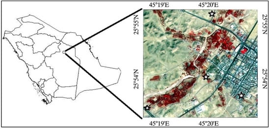
Figure 1.
Study area based on a false color composite of PS data; star represents the four Automatic Weather Stations (AWS) in the area.

Table 1.
Climate parameters for Majmaah region in 2021.
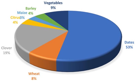
Figure 2.
The proportion of crops in Al-Majmaah.
2.2. Data Sources
PS high-resolution data, GRACE data, and climate data were used in this study. Except for the PS data, all these datasets are open to the public.
2.2.1. High-Resolution PS Data
PS reflectance imagery of 3 m spatial resolution with NIR and red bands was used to create the NDVI time series from January 2018 to December 2021 (Table 2). The false color composite of PS data for 3 December 2021, is shown in Figure 1. The vegetation is readily visible in red patches, whereas the other land cover classes or no vegetation are shown in cyan color. High spatiotemporal resolution of 3 m and one day makes PS an ideal dataset to analyse near real-time precision agriculture decision-making.
Table 2.
List of PS Satellite images used in the current investigation.
2.2.2. GRACE Data
GRACE and GRACE-FO satellites provided data on terrestrial water storage (TWS) from April 2002 to April 2021 at 0.5° geographical and monthly temporal resolutions. In this study, GRACE release 06 mascon products were used. They were obtained from CSR (the University of Texas at Austin’s Center for Space Research) and Jet Propulsion Laboratories (JPL).
2.2.3. Climate Data
The monthly minimum and maximum temperature data in °C (Tmin, Tmax), humidity (%), wind (km/day), and rainfall dataset (in mm) of four AWS were collected from January 2018 to December 2021 (Figure 3). The sun hours data were collected from the National Renewable Energy Laboratory (NREL) website (https://www.nrel.gov/gis/solar-geospatial-data-tools.html; accessed on 10 June 2022). The high resolution of the AWS dataset’s temporal availability provides an opportunity to calculate the reference ETo and radiation. The data is interpolated using the kriging method for monthly climate anomalies from four AWS. The CROPWAT model uses USDA and dependable rain methods to obtain effective rainfall estimates. In water-scarce areas, the USDA method is better, while the dependable rain method is better for water-sufficient areas; therefore, the monthly effective rainfall was calculated based on the USDA method [3].
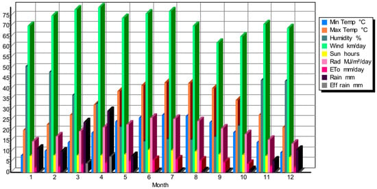
Figure 3.
Monthly climatic variables in the study area from January 2018–December 2021.
2.2.4. Soil and Crop Information Data
The soil moisture data were collected using Lutron PMS-714 m from January 2021 to December 2021 between the 20th and 30th day of each month. Except for dates acquired from the FAO dataset [17], the rooting depth of each crop was evaluated using five random samples. Equation (1) was used to compute the Soil Moisture Depletion (SMD) using the FAO model.
The FAO catalogue provided soil texture, maximum infiltration rate, and crop planting and harvesting dates. The mean vegetation harvesting area was determined using NDVI data from January 2018 to December 2021.
2.3. Methodology
Two methods were used to estimate the CWR in the study area: first, high-resolution PS data, and second, the FAO CROPWAT model v8.0. Figure 4 depicts the recommended methodology.
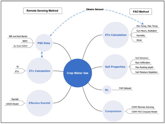
Figure 4.
The methodology used in the present investigation.
2.3.1. Calculation of Reference Evapotranspiration (ETo)
The calculation of ETo was the most important criterion for both techniques. Equation (2) shows the Penman–Monteith method, which was used to calculate reference evapotranspiration.
where, SH = density of soil heat flux, T = air temperature, Rn = net radiation, w = wind speed, ∆ = slope of vapor pressure curve, esv − eav = saturation vapor pressure deficit, γ = psychrometric constant.
The effective rainfall () was obtained from the FAO method [3] using Equation (3).
where is the total rainfall (mm). This method is valid where for a rainfall of Ptot < 250 mm.
2.3.2. CWR Estimation Using PS High-Resolution Remote Sensing
The ETo calculated in Section 2.3.1 was used with PS data to calculate the CWR. The availability of 4 AWS stations in the study area with recent climatic data provided a good opportunity to calculate the CWR. To obtain the CWR based on PS data requires the NDVI and Kc estimation, which is given in the following sections.
NDVI
The NDVI index measures plant “greenness” or photosynthetic activity [15,18,19]. The NDVI method was developed on the assumption that plants absorb the red light, which is required for photosynthesis, but reflect near-infrared (NIR) light. In non-vegetated areas or stressed vegetation, the process is reversed, with red light reflected more and NIR light reflected less.
The NDVI is calculated by Equation (4) as follows:
Total vegetation cover, soil moisture, and vegetation stress are all factors that influence the NDVI. Because it is a ratio, NDVI has several advantages, including topographic lighting correction and multi-temporal image analysis for comparing images obtained at different seasons.
Estimation of Crop Coefficient (Kc)
The crop coefficients, Kc represent the crop type and the development of the crop. The Kc also relates to the crop evapotranspiration (ETc) and ETo ratio, which is critical when calculating ETo. The ground-truth data for measured Kc values are required to establish an NDVI-Kc connection. From January 2018 to December 2021, the extent of crops was determined using NDVI data. Based on the approach of Kamble et al. [20] and Mahmoud and Gan [5], Kc is determined using NDVI averaged data between 2018 and 2021. Twenty sampling locations from various fields and crops were chosen to check the NDVI computed from the PS dataset. A database of default Kc was created to use in the GIS environment. The database comprised seven crop types: date palm, wheat, clover, maize, barley, citrus, and vegetables. The FAO’s database [17] contains Kc values for crops as well as dates for the growing season. Kc is calculated using NDVI time-series data and linear regression given in Equation (5).
where is the response variable for xth case, …… were monthly NDVI and error term with mean zero value. The values and in Equation (5) are values that were calculated using least squares regression.
The coefficients in Equation (5) were calculated using seven different crop datasets and the date of the year during the growing season. The coefficient of determination (r2) denotes the percentage of variance assigned to the linear combination of the independent variables. For the linear model stated in Equation (5), the coefficient of determination was used to determine the Kc and NDVI relationship, as shown in Equation (6).
PS data’s high resolution (3 m) makes it an excellent alternative to computing Kc values at a high spatial resolution, which was a crucial concern in previous research that used the MODIS dataset for relatively small fields and had resolution issues [5,20].
ETc Calculations
The Kc values and ETo values were multiplied to get the ETc values for the study area based on Equation (7).
The monthly maps were developed from January 2018 to December 2021 to obtain the CWR for the study period.
Site Selection
Twenty crop fields were selected and extracted from NDVI maps for each month from January 2018 to December 2021 to study the pattern of NDVI, Kc, and ETc.
2.3.3. CWR Estimation using CROPWAT 8.0 Model
Smith (1991) developed the CROPWAT software, which can calculate crop water needs, and irrigation requirements for various crops, and reference ETo. The FAO developed the most recent version of CROPWAT v.8. It includes a sample water balance model that includes yield reduction calculations and water stress condition simulations and is based on well-established ETc approaches [21]. CROPWAT is a helpful tool for planning irrigation under various management systems and scheme supplies and assessing irrigation application efficiency and rain-fed production. Both meteorological and crop data are required as inputs to CROPWAT. CLIMWAT is a climatic database that works with the CROPWAT to calculate crop water requirements, with climatological stations for 144 nations; however, the spatial grid size is too large for sparse and small crop areas. The local AWS data were utilized to calculate the ETo, CWR, and irrigation water requirement (IWR). Monthly ETo was calculated using Equation (2). The monthly ETo values and Kc values were multiplied to get the CWR. Equation (8) was used to calculate the irrigation water requirement (IWR).
where E = actual crop evapotranspiration; = the effective rainfall; c = crop index; = actual evapotranspiration and Ac = cultivated area. The value of the effective rainfall was obtained using Equation (3).
The program includes a cropping pattern with the planting date, Kc data, growing and harvesting dates, and the area planted (0–100% of the total area). The total area of crops was derived using the NDVI model.
The soil moisture deficit threshold is required to compute an irrigation schedule. The limit of Readily Available Moisture (RAM) in the soil is the critical level when the crop gets stressed, see Equation (9).
where TAM is total available moisture in the soil, measured in millimeters of water per meter in soil thickness, see Equation (10).
An ideal irrigation plan will never strain the crop, and no water will be lost due to over-irrigation. Water use will be lowered while crop yield will not be affected. The “F” threshold is the upper limit with a 40–60% typical value. Because the crop root depth increases as the season advances and the crop grows, the TAM and RAM will likewise increase.
2.3.4. GRACE Processing
GRACE is unable to distinguish anomalies from numerous TWS elements on its own. The soil moisture content (SMC) must be deducted from the change in terrestrial water storage (TWS) to calculate the change in groundwater storage (GWS) [22]. See Equation (11).
2.3.5. Trend and Correlation Analysis
Mann–Kendall trend tests were carried out for trend analysis to detect trends and changes in vegetation, GWSC, and climate variables over the years of analysis. Sen’s slope values were used to understand the trend of all parameters from January 2018 to October 2021. Equations (12)–(15) define the trend tests and slope value computation.
3. Results and Discussion
3.1. CWR Estimation Using PS High-Resolution Remote Sensing
The CWR estimated using the remote sensing method is given stepwise in NDVI, Kc, CWR, and IWR results analysis.
3.1.1. NDVI Analysis
The largest vegetation area in the observation period was recorded in December 2018, and the lowest vegetation area was detected in April 2020 (Figure 5 and Figure 6).
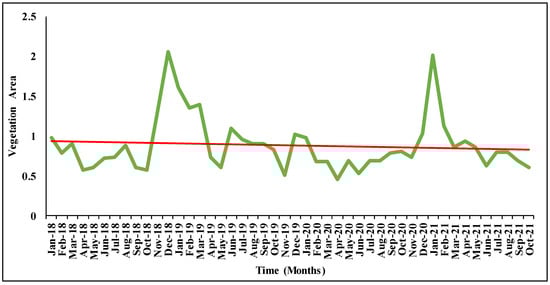
Figure 5.
Vegetation area in Al Majmaah region from January 2018–October 2021.
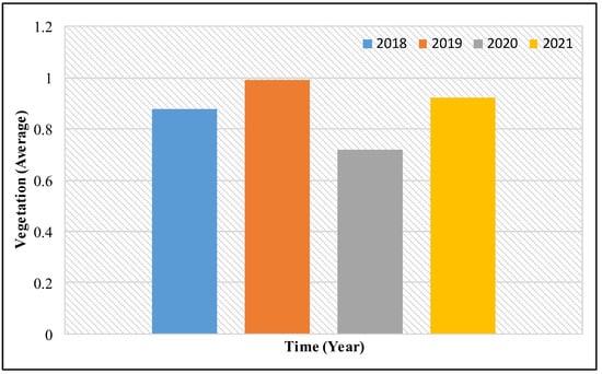
Figure 6.
Vegetation Area in Majmaah from January 18 to October 2021.
Vegetation area peaks were seen for 2019 and 2021 for December and January. The year 2020 had a lower annual mean vegetation area than the other three years, namely 2018, 2019, and 2021. Low vegetation is present from March 2019 to August 2020. The COVID-19 pandemic effect and reduced rainfall in 2019 were the fundamental causes of this low agricultural output. For better visualization, the NDVI images were divided into four categories: no vegetation from −1 to 0.15, low vegetation from 0.15 to 0.30, medium vegetation from 0.30 to 0.45, and high vegetation from 0.45 and above (Figure 7). The NDVI values in May 2020 were the highest of any month. For all three years of research, the NDVI of November, December, and January were more significant than other months. However, there was less vegetation in April, May, and September. The wheat cycle was shown to be highly linked with the NDVI data.
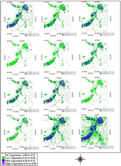
Figure 7.
Monthly NDVI maps for Al Majmaah from January 2018 to December 2018 (left to right and top to bottom).
Previous studies revealed that NDVI curves were found to have low values in the early parts of the season, then steadily climbed from the beginning to the middle of the season, then remained constant until the end. The high resolution of PS data allows more exact measurements that are less influenced by pixel spectrum mixing. In SA, the date is a significant crop, particularly in Al-Majmaah; it is a perennial crop. Harvesting occurs between July and August, and the dates are highly connected with the NDVI images. The CWR for November 2018 exhibited a negative CWR for the river region (in black) with water after rainfall; thus, this RS-based CWR can capture environmental pattern changes such as rainfall and is highly connected with temperature. The NDVI curves of 20 selected fields of Al Majmaah for the observation period are shown in Figure 8. The NDVI curves for 2018 and 2021 are almost similar for all 20 fields.
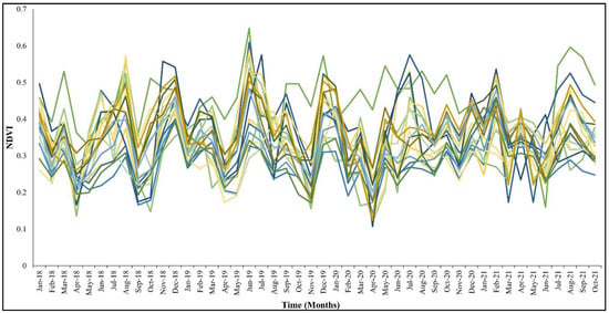
Figure 8.
Monthly changes in NDVI for twenty crop fields in Al Majmaah from January 2018 to October 2021 (Each color line shows a specific field).
3.1.2. Kc Analysis
Crop factors such as crop area and planting dates were used to create monthly Kc maps for Al Majmaah (Figure 9). Figure S1 shows the average monthly Kc for all crops for the 20 sites.
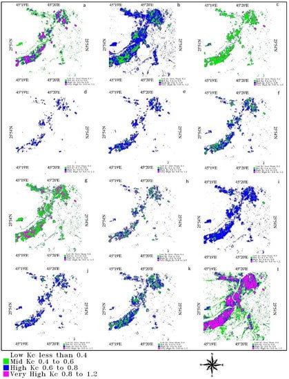
Figure 9.
Monthly averaged Kc maps for Al Majmaah from January 2018 to December 2018 (left to right and top to bottom). The months are represented from (a–l) for January–December.
The monthly averaged Kc value curves for all crops and the monthly NDVI curves showed a similar pattern. Monthly linear regression models were developed to find the link between NDVI and averaged Kc for the selected 20 sites to quantify this relationship (Figure 10).
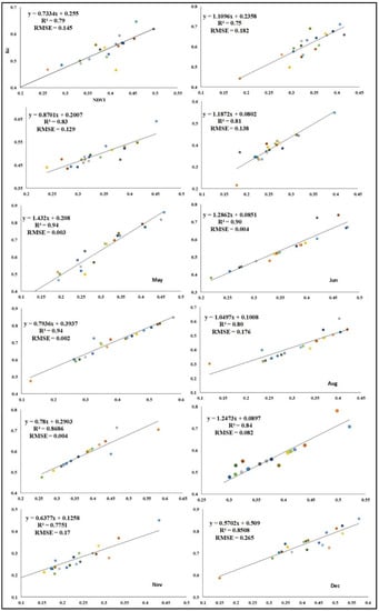
Figure 10.
Month-wise relationship between NDVI and averaged Kc for selected 20 fields in Al Majmaah.
The R2 values for monthly regression models of Kc and NDVI ranged from 0.75 to 0.94. The highest R2 value of 0.94 was observed for May and July, with RMSE values of 0.003 and 0.002, respectively. The least R2 value of 0.75 with an RMSE value of 0.145 was observed for Jan. The change in R2 values was due to the vegetation seasons for different crops, which exhibit low relation during more vegetation and comparatively higher R2 values in low vegetation time. The regression models developed in the current investigation were comparable with previous studies.
3.1.3. CWR Analysis
Monthly CWR maps for Al Majmaah were created using the monthly Kc estimated in the earlier section and ETo calculated using the environmental dataset (Figure 11). CWR maps were categorized into five categories: ≤40, 40–60, 60–80, 80–100, and ≥100. According to the CWR maps, the summer months of June, July, and August require the most water for crops, while the winter months require the least. It was clear that the higher temperature and lack of rainfall in summer months necessitated more water for crops, whereas winters get rainfall and the relatively lower temperatures mean that less water is required for crops.
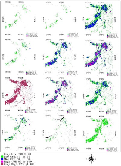
Figure 11.
Monthly CWR maps for Al Majmaah from January 2018 to December 2018 (left to right and top to bottom).
In July, the CWR for the maximum area was greater than 100 (Figure 11). Al-Majmaah received very high rainfall in November 2018 This is also indicated in Figure 11, which depicts the water channel in black as a negative CWR due to water-filled channels and surrounding agricultural areas. Figure S2 shows the monthly CWR trends for 20 sites from January 2018 to October 2021. CWR peaks were recorded in all four years throughout the summer months, with less CWR in April 2020 due to less vegetation during COVID-9-related lockdowns.
3.1.4. IWR Analysis
Figure S3 depicts the monthly IWR trends for 20 sites from January 2018 to October 2021. The difference between CWR and effective rainfall was used to calculate the IWR. IWR curves followed a similar pattern to CWR curves, with peaks in the summer months and less irrigation required in the winter months.
3.2. CWR Estimation Using CROPWAT 8.0 Model
CROPWAT 8.0 was used to calculate the CWR values of seven crops for Al-Majmaah, including date palm, wheat, citrus, maize, barley, clover, and vegetables (Figure 12).
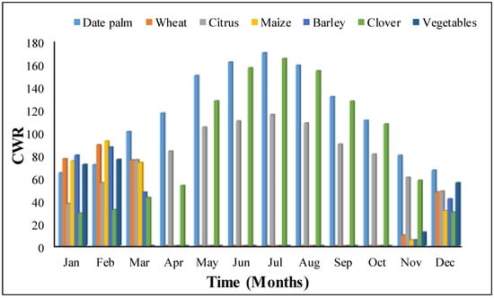
Figure 12.
CWR estimation of seven crops using CROPWAT 8.0 for Al Majmaah.
The annual CWR (in mm) for the seven crops evaluated in this study were 1377, 296, 964, 275, 259, 1077, and 214 for date palm, wheat, citrus, maize, barley, clover, and vegetables, respectively. Due to their perennial nature, date palm, citrus, and clover can be found throughout the year (Figure 12). CWR requirements were found in wheat, maize, barley, and vegetables between November and March. CROPWAT model-based CWR confirms the PS-based dataset showing the highest CWR requirements for July. In July, the date, clover, and citrus plants required 170 mm, 164 mm, and 115 mm of CWR, respectively. Figure 13 depicts a separate CWR for all seven crops.
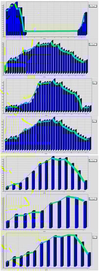
Figure 13.
CWR estimation for Al Majmaah using CROPWAT model for all seven crops.
Optimal Irrigation Schedules
Efficient use of available water resources needs management systems that adapt to changing environments in the semi-arid region of Al-Majmaah, SA. The CROPWAT model was used to calculate the best irrigation schedules for all seven crops (Figure 14). The best irrigation schedule saves water while also maximizing the irrigation rate in a timely and cost-effective manner. It recommends the best irrigation practices for a given region based on meteorological and soil factors.
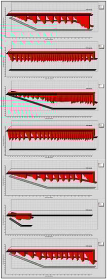
Figure 14.
Optimized irrigation schedules for Al Majmaah using CROPWAT model for all seven crops.
3.3. Groundwater Change Using GRACE Dataset
An attempt has been made to examine GWS change using the GRACE and GRACE-FO datasets for Al-Majmaah (Table 3). The CSR-based GWS trend revealed a rapid rate of water depletion. GWS based on JPL, on the other hand, showed far less depletion (Figure 15). Similar observations were made by others [15,22]. The important aspect to note is that GRACE’s spatial resolution is relatively coarse (~400 km) and has a combined multitude of parameters. Thus, it may be overestimating the values for a region such Al-Majmaah.
Table 3.
Change analysis using Kendall’s tau and Sen’s slope with (95% confidence interval and α = 0.05).
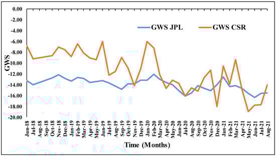
Figure 15.
GWS change from June 2018–August 2021 based on JPL and CSR data processing.
3.4. Trend and Correlation Analysis of CWR, Kc, Climatic Variables, and GRACE Dataset
The analysis revealed that ETo showed a minimum response of 2.22 mm/day in January to a maximum of 6.13 mm/day in July, with high temperatures (42.8 °C). The humidity reaches its peak of 51%, then falling to a minimum in June of 15% (Figure S4). The long-term trend of rainfall and temperature for Al Majmaah from January 1981–December 2020 based on CRUTS version 4.0.5 data shows decreasing and increasing trends, respectively (Figure 16 and Figure 17).
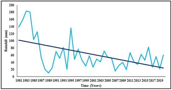
Figure 16.
Long-term trend of rainfall for Al Majmaah from January 1981–December 2020 based on CRUTS version 4.0.5 data. The x-axis represents years, and the y-axis represents annual rainfall in mm.
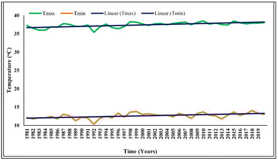
Figure 17.
Long-term trend of temperature for Al Majmaah from January 1981–December 2020 based on CRUTS version 4.0.5. The x-axis represents years, and the y-axis represents the Tmin and Tmax in °C.
3.5. Correlation Analysis
The effect of climatic variables such as temperature and rainfall on vegetation has been investigated (Figure 18).
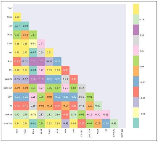
Figure 18.
Correlation plot between annual climatic parameters, GWS based on JPL, CSR, and a mean value, NDVI, Kc, CWR, IWR.
All of the parameters have significant correlations with each other, with a strong correlation between them. For the combined four years, an interesting association (r = 0.81) was observed between CWR computed using PS Satellite data and CROPWAT 8.0. The CROPWAT model results have a higher correlation (r = 0.83) with the monthly averaged CWR calculated using PS (Figure 19 and Figure 20). The most recent identical climate data to estimate ETo and the efficacy of high-resolution PS data to extract the finer vegetation characteristics could be the main reasons for this good match.
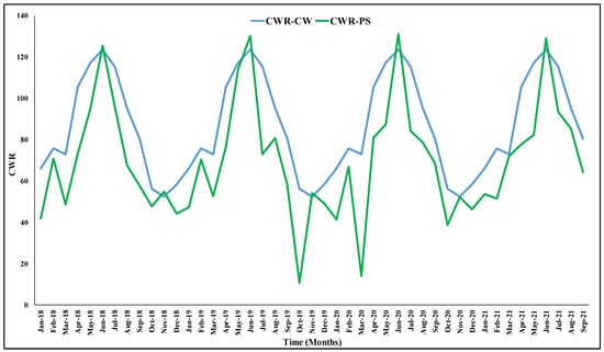
Figure 19.
CWR estimation for Al Majmaah using CWR-PS and CWR-CW from January 2018–October 2021.
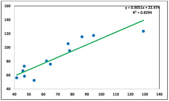
Figure 20.
Correlation of CWR derived using PS data and FAO CROPWAT model.
4. Comparison with Other Studies
There are five major aquifers in SA, namely Saq, Wajed, Minjur, Um Rudimah, and Wasea [22]. The Saq aquifer is one of the largest and most well-documented aquifers in the SA [23,24,25,26,27,28,29,30]. The area monitored in the present study used groundwater from Minjur aquifer for agriculture. Haq [22] observed a decreasing trend of GWS for the Minjur aquifer with a value of −5.9 + 1.5 mm/year based on JPL-GWS and CSR-GWS from 2003 to 2020. However, utilizing JPL-GWS and CSR-GWS from 2003 to 2020, the present study found a much smaller drop of −0.331.4 mm/year and −2.661.4 mm/year. It depicts the sustainable use of water for agriculture in the Majmaah region. Haq [15] observed a decreasing trend of GWS for the Qaseem region with a value of greater than 10.3 + 1.4 mm/year based on JPL-GWS and CSR-GWS from 2003 to 2020.
Previous studies [13,14,20,31] utilized either CROPWAT or the Remote Sensing approaches for CWR estimation. However, earlier studies did not discuss the link between the Remote Sensing-based CWR and the CROPWAT model-based CWR. The novelty of the present study was to use high-resolution PS data and compute the CWR based on the remote sensing method, comparing it with CROPWAT based CWR.
The regression models developed in this study were equivalent to those used in previous studies. According to Mahmoud and Gan [13], monthly R2 values between Kc and NDVI ranged from 0.72 to 0.95. Mahmoud and Gan [13] employed soil characteristics, gridded water-holding capacity, and MOD13A2 data to create Kc and NDVI regression models with spatial resolutions of 40 × 40 km, 28 × 28 km, and 1 × 1 km for the Al-Qaseem region. The mean area of pivot agricultural fields in Al-Qaseem is roughly 0.5 km2, which is substantially less than the dataset used by Mahmoud and Gan [13], making it subjective for precise modeling of the relationship between Kc and NDVI (Jia et al., 2021). On the other hand, to cover a greater area, coarse resolution data can be used for computation. Precision agricultural analysis using high-resolution data is very useful; however, the complexity of details was noted, especially for higher resolution datasets [32].
A well-known study [20] found that combining MODIS NDVI and Kc yielded a combined regression model with an R2 value of 0.82. The combined model has a similar R2 value in the current investigation. Equations (16) and (17) show the integrated model of Kamble et al. [20] with the current investigation.
where x = NDVI and y = Kc.
Kamble et al. [20] used MODIS data for NDVI and AmeriFlux data for Kc for three different locations in the USA, including desert and mountain agriculture.
Another study was performed by El-Shirbeny et al. [10]. They used Landsat 8 data and developed a regression model between Kc and NDVI as per Equation (18).
Landsat 8’s 30 m spatial resolution makes it an excellent choice for analyzing vegetation and crop requirements for scattered and smaller fields, which are common in dry and semi-arid environments. The only problem with the Landsat data is the 16-day temporal resolution. However, the PS data used in this study has a 1-day temporal resolution and a spatial resolution of 3 m, making it a viable candidate for precision agriculture.
Another study conducted by Reyes-González et al. [11]. They used 27 Landsat 7 and 8 images acquired between 2013 and 2016 to analyze Kc and NDVI for CWR in the Northern Mexico area, as in Equation (19).
Reyes-González et al. [11] found a good relationship between Kc and NDVI, with an R2 value of 0.97. The number of fields considered for the regression model was five in total, which was a key point of subjectivity in the Reyes-González et al. [11] study. Another significant difficulty was using Landsat 7 data, which has a problem with off SLC. The normalization of this effect requires a mean filter to fill the no data values. Due to a shortage of clear sky images during the growing seasons, the NDVI curves were incomplete [11].
Aragon et al. [33] combined a high-resolution CubeSat dataset with the Priestley–Taylor’s Jet Propulsion model developed by Fisher et al. [34]. This model is based on the Penman–Monteith model, with some downscaling of evapotranspiration into the different canopy and soil subcomponents. The choice of parameters such as sensitivity β = 3, A = 0.31, k, Rn = 0.6, m2 = 1, and b2 = −0.05 makes this model a little more complicated to use for calculating all parameters obtained for the global context utilizing AVHRR (1 km).
Khan et al., [12] used the CROPWAT 8.0 model to estimate CWR for five crops in the Al-Qaseem region: rice, citrus, maize, wheat, and barley. The climate data used in Khan et al. [12] is similar to that of Abbas Abdullah [35], which was taken from CLIMWAT dataset till 2011. CLIMWAT was a large worldwide climate dataset with over 5000 stations from 1971 to 2000 [21]. The climatic parameters are a dynamically changing phenomenon, and the current characteristics such as ETo, temperature, and rainfall used from historical data from 1971–2000 are prone to subjectivity when applied to the current context. Another problem identified by Khan et al. [12] was the rice crop, which was essentially non-existent outside of the Al-Ahsa region, known for its red rice. Saudi Arabia’s rice production has decreased from 2800 tons in 1961 to 0 tons in 2019. This is due to water conservation guidelines.
The COVID-19 pandemic allows us to analyze system-wide changes in water, energy, and food (WEF) [23]. The examination of COVID-19’s impacts on the CWR showed a decrease from April 2020 due to less vegetation during COVID-9-related lockdowns.
5. Conclusions
The goal of this study was to figure out how to calculate CWR using remote sensing and the FAO’s CROPWAT model. The annual CWR (in mm) for the seven crops evaluated in this study were 1377, 296, 964, 275, 259, 1077, and 214 for date palm, wheat, citrus, maize, barley, clover, and vegetables, respectively. From January 2018 to November 2021, the current study found a slight rise in vegetation, CWR, and IWR. The increase in tree growth, which necessitates more water for date crops, is the primary cause. The GWS trend indicated a downward trend, whereas the temperature trend was upward.
The monthly averaged CWR calculated using PS and the CROPWAT model had a greater correlation (r = 0.83) in the current study. The efficiency of high-resolution PS data to get the finer vegetation details may be the fundamental explanation for this good correlation. We utilized the most recent identical climatic data to estimate ETo and the efficiency of high-resolution PS data to get the finer details of vegetation. CWR was generated using four years of high-resolution data in this study. Furthermore, the availability of daily PS satellite data with a very high temporal resolution can provide CWR at a daily resolution, which is particularly useful for near real-time water management decision-making in sustainable agriculture. The future scope of the present investigation is to use advanced deep learning models [36,37] to predict the CWR based on high-resolution satellite data and climate data.
Supplementary Materials
The following supporting information can be downloaded at: https://www.mdpi.com/article/10.3390/su142013554/s1.
Author Contributions
Conceptualization, M.A.H.; methodology, M.A.H.; software, M.A.H.; writing—original draft preparation, M.A.H. and M.Y.A.K.; writing—review and editing, M.A.H. and M.Y.A.K.; supervision, M.Y.A.K.; funding acquisition, M.Y.A.K. All authors have read and agreed to the published version of the manuscript.
Funding
The Deanship of Scientific Research (DSR) at King Abdulaziz University, Jeddah, Saudi Arabia has funded this project, under grant no. D-410-145-1443.
Institutional Review Board Statement
Not applicable.
Informed Consent Statement
Not applicable.
Data Availability Statement
Not applicable.
Acknowledgments
The authors gratefully acknowledge technical and financial support provided by the Deanship of Scientific Research (DSR) at King Abdulaziz University, Jeddah, Saudi Arabia.
Conflicts of Interest
The authors declare no conflict of interest.
References
- Hussein, H. Lifting the veil: Unpacking the discourse of water scarcity in Jordan. Environ. Sci. Policy 2018, 89, 385–392. [Google Scholar] [CrossRef]
- Food and Agriculture Organization (Fao) of the United Nations. Groundwater Management in Saudi Arabia. Draft Synthesis Report; FAO: Rome, Italy, 2009; p. 14. [Google Scholar]
- Gabr, S.S.; Morsy, E.A.; El Bastawesy, M.A.; Habeebullah, T.M.; Shaaban, F.F. Exploration of potential groundwater resources at Thuwal area, north of Jeddah, Saudi Arabia, using remote sensing data analysis and geophysical survey. Arab. J. Geosci. 2017, 10, 509. [Google Scholar] [CrossRef]
- Abderrahman, W.A. Groundwater Resources Management in Saudi Arabia Special Presentation at Water Conservation Workshop; Saudi Arabian Water Environment Association: Khober, Saudi Arabia, 2006. [Google Scholar]
- Khan, M.Y.A.; El Kashouty, M.; Gusti, W.; Kumar, A.; Subyani, A.M.; Alshehri, A. Geo-Temporal Signatures of Physicochemical and Heavy Metals Pollution in Groundwater of Khulais Region—Makkah Province, Saudi Arabia. Front. Environ. Sci. 2022, 9, 1–22. [Google Scholar] [CrossRef]
- Al-Ibrahim, A.A. Excessive use of groundwater resources in Saudi Arabia: Impacts and policy options. Ambio 1991, 20, 34–37. [Google Scholar]
- Haq, M.A.; Rahaman, G.; Baral, P.; Ghosh, A. Deep Learning Based Supervised Image Classification Using UAV Images for Forest Areas Classification. J. Indian Soc. Remote Sens. 2021, 49, 601–606. [Google Scholar] [CrossRef]
- Haq, M.A.; Rahaman, G.; Baral, P.; Avantika, S. Comparison of Machine Learning Classification Algorithms for Crops Identification Using Sentinel-2A Data Sets. In Proceedings of the IEEE SSCI, Symposium Series on Computational Intelligence, Bangalore, India, 18–21 November 2018. [Google Scholar]
- Manjula, A.; Narsimha, G. XCYPF: A flexible and extensible framework for agricultural Crop Yield Prediction. In Proceedings of the 2015 IEEE 9th International Conference on Intelligent Systems and Control (ISCO 2015), Coimbatore, India, 9–10 January 2015. [Google Scholar]
- El-Shirbeny, M.A.; Ali, A.-E.M.; Saleh, N.H. Crop Water Requirements in Egypt Using Remote Sensing Techniques. J. Agric. Chem. Environ. 2014, 3, 57–65. [Google Scholar] [CrossRef]
- Reyes-González, A.; Kjaersgaard, J.; Trooien, T.; Hay, C.; Ahiablame, L. Estimation of Crop Evapotranspiration Using Satellite Remote Sensing-Based Vegetation Index. Adv. Meteorol. 2018, 2018, 4525021. [Google Scholar] [CrossRef]
- Khan, W.A.; Rahman, J.U.; Mohammed, M.; AlHussain, Z.A.; Elbashir, M.K. Topological sustainability of crop water requirements and irrigation scheduling of some main crops based on the Penman-Monteith method. J. Chem. 2021. [Google Scholar] [CrossRef]
- Mahmoud, S.H.; Gan, T.Y. Irrigation water management in arid regions of Middle East: Assessing spatio-temporal variation of actual evapotranspiration through remote sensing techniques and meteorological data. Agric. Water Manag. 2019, 212, 35–47. [Google Scholar] [CrossRef]
- De Oliveira, T.C.; Ferreira, E.; Dantas, A.A.A. Variação temporal do índice de vegetação por diferença normalizada (NDVI) e obtenção do coeficiente de cultura (Kc) a partir do NDVI em áreas cultivadas com soja irrigada. Cienc. Rural. 2016, 46, 1683–1688. [Google Scholar] [CrossRef][Green Version]
- Haq, M.A. Intellligent sustainable agricultural water practice using multi sensor spatiotemporal evolution. Environ. Technol. 2021, 1–14. [Google Scholar] [CrossRef]
- Alharbi, T. Establishment of natural radioactivity baseline, mapping, and radiological hazard assessment in soils of Al-Qassim, Al-Ghat, Al-Zulfi, and Al-Majmaah. Arab. J. Geosci. 2020, 13, 415. [Google Scholar] [CrossRef]
- Food and Agriculture Organization of the United Nations FAO. FAO Publications Catalogue 2021; FAO: Rome, Italy, 2021. [Google Scholar] [CrossRef]
- Haq, M.A.; Baral, P.; Yaragal, S.; Rahaman, G. Assessment of trends of land surface vegetation distribution, snow cover and temperature over entire Himachal Pradesh using MODIS datasets. Nat. Resour. Model. 2020, 33, e12262. [Google Scholar] [CrossRef]
- Shoab, M.; Haq, M.A. Development of Field GIS Data Collection Tool for Smartphones. International Symposium on Mobile Mapping Technology. In Proceedings of the International Symposium on Mobile Mapping Technology (MMT 2013), Tainan, Taiwan, 29 April–3 May 2013; p. 6. [Google Scholar]
- Kamble, B.; Kilic, A.; Hubbard, K. Estimating crop coefficients using remote sensing-based vegetation index. Remote Sens. 2013, 5, 1588–1602. [Google Scholar] [CrossRef]
- FAO. (n.d.). CLIMWAT|Land & Water|Food and Agriculture Organization of the United Nations|Land & Water|Food and Agriculture Organization of the United Nations. Available online: https://www.fao.org/land-water/databases-and-software/climwat-for-cropwat/en/ (accessed on 27 December 2021).
- Haq, M.A.; Khadar Jilani, A.; Prabu, P. Deep Learning Based Modeling of Groundwater Storage Change. Comput. Mater. Contin. 2022, 70, 4599–4617. [Google Scholar] [CrossRef]
- Al-Saidi, M.; Hussein, H. The Water-Energy-Food Nexus and COVID-19: Towards a Systematization of Impacts and Responses. Sci. Total Environ. 2021, 779, 146529. [Google Scholar] [CrossRef]
- Ferragina, E.; Greco, F. The Disi Project: An Internal/External Analysis. Water Int. 2008, 33, 451–463. [Google Scholar] [CrossRef]
- Greco, F. The Securitization of the Disi Aquifer: A Silent Conflict between Jordan and Saudi Arabia Disi Is; London Water Research Group: London, UK, 2005. [Google Scholar]
- Greenwood, R. Social, Political, Economic and Health Effects of the Disi Aquifer on Jordanian Society. 2011. Available online: http://digitalcollections.sit.edu/isp_collection/1104 (accessed on 10 June 2022).
- Hussein, H. Yarmouk, Jordan, and Disi Basins: Examining the Impact of the Discourse of Water Scarcity in Jordan on Transboundary Water Governance. Mediterr. Politics 2019, 24, 269–289. [Google Scholar] [CrossRef]
- Jasem, A.F.; Shammout, M.; AlRousan, D.; AlRaggad, M. The Fate of Disi Aquifer as Stratigic Groundwater Reserve for Shared Countries (Jordan and Saudi Arabia). J. Water Resour. Prot. 2011, 3, 711–714. [Google Scholar] [CrossRef][Green Version]
- Qtaishat, T. Water Policy in Jordan BT. In Water Policies in MENA Countries; Springer: Cham, Swizerland, 2020. [Google Scholar] [CrossRef]
- Salameh, E.; Alraggad, M.; Tarawneh, A. Disi Water Use for Irrigation—A False Decision and Its Consequences. Clean-Soil Air Water 2014, 42, 1681–1686. [Google Scholar] [CrossRef]
- Basiri, A.F. Options for Improving Irrigation Water Allocation and Use: A Case Study in Hari Rod River Basin, Afghanistan; LAP LAMBERT Academic Publishing: Chisinau, Moldova, 2009. [Google Scholar]
- Jia, D.; Cheng, C.; Song, C.; Shen, S.; Ning, L.; Zhang, T. A hybrid deep learning-based spatiotemporal fusion method for combining satellite images with different resolutions. Remote Sens. 2021, 13, 645. [Google Scholar] [CrossRef]
- Aragon, B.; Houborg, R.; Tu, K.; Fisher, J.B.; McCabe, M. Cubesats enable high spatiotemporal retrievals of crop-water use for precision agriculture. Remote Sens. 2018, 10, 1867. [Google Scholar] [CrossRef]
- Fisher, J.B.; Tu, K.P.; Baldocchi, D.D. Global estimates of the land-atmosphere water flux based on monthly AVHRR and ISLSCP-II data, validated at 16 FLUXNET sites. Remote Sens. Environ. 2008, 112, 901–919. [Google Scholar] [CrossRef]
- Abbas, A. Implications of Climate Change on Crop Water Requirements in Saudi Arabia. [King Fahd University of Petroleum and Minerals]. 2013. Available online: https://eprints.kfupm.edu.sa/id/eprint/139133/1/Thesis_Abbas.pdf (accessed on 10 June 2022).
- Haq, M.A. CDLSTM: A Novel Model for Climate Change Forecasting. Comput. Mater. Contin. 2022, 71, 2363–2381. [Google Scholar]
- Haq, M.A. SMOTEDNN: A Novel Model for Air Pollution Forecasting and AQI Classification. Comput. Mater. Contin. 2022, 71, 1403–1425. [Google Scholar]


Publisher’s Note: MDPI stays neutral with regard to jurisdictional claims in published maps and institutional affiliations. |
© 2022 by the authors. Licensee MDPI, Basel, Switzerland. This article is an open access article distributed under the terms and conditions of the Creative Commons Attribution (CC BY) license (https://creativecommons.org/licenses/by/4.0/).