Abstract
The interaction among social economy, geography, and environment leads to the occurrence of traffic accidents, which shows the relationship between time and space. Therefore, it is necessary to study the temporal and spatial correlation and provide a theoretical basis for formulating traffic accident safety management policies. This paper aims to explore the traffic accident patterns in 31 provinces of China by using statistical analysis and spatial clustering analysis. The results show that there is a significant spatial autocorrelation among traffic accidents in various provinces and cities in China, which means that in space, the number of traffic accidents and deaths is high with high aggregation and low with low aggregation. Positive spatial autocorrelation is primarily concentrated in the southeast coastal areas, while negative spatial autocorrelation is mainly concentrated in the western areas. Jiangsu, Anhui, Fujian, and Shandong are typical areas of traffic accidents, which deviate from the overall positive spatial autocorrelation trend. Traffic accidents in Sichuan are much more serious than those in neighboring provinces and cities; however, in recent years, this situation has disappeared.
1. Introduction
Traffic injuries are one of the leading causes of death worldwide, and their ranking among all causes of death has been climbing steadily [1]. In addition, as one of the primary public health issues worldwide, road traffic safety is considered a “hidden pandemic,” which has become another significant cause of human death after diseases as heart disease and cancer. According to statistics, the elderly account for the majority of those who die from the disease, but young adults aged 16–40 account for the majority of traffic deaths; so, from this perspective, traffic accidents are more severe than fatal diseases. In concrete terms, traffic accidents kill approximately 1.2 million people and injure over 50 million people each year [2], implying that one person dies in traffic accidents every 24 s, making it even more deadly than tuberculosis. However, this situation also differs between developed countries and developing countries. With increased urbanization and motorization, the number of road traffic accidents has also increased dramatically, with developing countries having the highest annual road death rate. Specifically, developing countries have 72 percent of the world’s population and 52 percent of the world’s registered vehicles, but the number of road traffic deaths accounts for as high as 80 percent of the world’s total [3]. Furthermore, whether in developed or developing countries, traffic accidents have a significant impact on the GDP (Gross Domestic Product). The economic cost of traffic accidents in developing countries is much higher than in developed countries [4], and traffic accidents account for 2–3 percent of the country’s GDP in developing countries [5].
China’s road traffic business is also developing rapidly, with China’s economic development and the increasing need for travel. According to statistics, the number of motor vehicles, drivers, and road mileage in China has continuously increased in recent years. From the end of 2019 to the end of 2020, the number of civil and private cars in China increased by 19.64 million and 17.82 million, respectively, over the previous year. At the same time, China’s highways and expressways increased by 18.56 thousand km and 11.40 thousand km, respectively, over the previous year. Moreover, the road density increased by 1.94 km per 100 sq km compared with the previous year. Along with the rapid development of China’s road traffic, road density continues to escalate, and the situation regarding road traffic safety is still serious. According to the latest report by Xinhua, the number of road traffic accidents in China has been declining in recent years, but it is also noteworthy that China’s annual road traffic accident death toll is still the second highest in the world [6]. In addition, there were over 11.43 million traffic accidents and more than 2.69 million deaths in China in the past 22 years, which is equivalent to the elimination of a medium-sized city. Furthermore, according to the report of Traffic Administration Bureau of the Chinese Ministry of Public Security (2019), there were more than 2.59 thousand children under the age of 15 killed in traffic accidents, and more than 19,600 children were injured in traffic accidents in 2019 alone, which is equivalent to seven children passing every day due to traffic accidents; it is obvious that road traffic accidents are still a danger to children. It is apparent that traffic accidents have been a major destabilizing factor, causing enormous losses for Chinese society and families. Therefore, as a developing country with a “strong transportation strategy,” China needs to ensure the safety of road traffic to realize strategic policy. Revealing the temporal and spatial distribution characteristics of road traffic accidents in China is of positive significance for deepening the risk cognition of road traffic accidents and can provide a theoretical basis for the government to formulate regional traffic management policies and construct corresponding control policies.
The research on road traffic accidents in China mainly focuses on these aspects: the severity of traffic accidents [7], factors related to the severity [8,9]; and economic factors related to traffic accidents [10], and forecast models, such as the SMEED model [11] and Markov chain model [12]. Nevertheless, it is insufficient to use traditional research methods to analyze traffic accidents, and we urgently need to know the relationship between traffic accidents in different regions and at different times so as to formulate effective traffic accident control policies according to local conditions.
Traffic accidents occur frequently, which can be studied by dividing data samples in time and space [13]. According to previous studies, many factors lead to traffic accidents, such as the economy, weather, and travel activities with time characteristics, meaning the occurrence of traffic accidents also has a time correlation [14]. In addition, other factors affecting traffic accidents include road facilities, geographical terrain, and the traffic environment. Hence, traffic accidents also have spatial characteristics [10].
Among the many new methods and tools, GIS has absolute advantages in analyzing the temporal and spatial characteristics of road traffic accidents, which are widely used. GIS can research the spatial distribution characteristics of traffic accidents based on visualization. GIS can determine the hot spots of road traffic accidents based on visualization [15,16] and mine traffic black spots [17] to study traffic accidents and their spatial distribution characteristics [18]. Additionally, based on GIS visualization, it was found that the research methods of density analysis and cluster analysis have a good effect on determining the spatial distribution characteristics of road traffic accidents [19].
In addition to these visualization methods, the time-based modeling method is also very effective for studying the temporal characteristics of traffic accidents, which includes the spatial error generalized ordered logit model [20], the spatial intermediate generalized ordered response probit model [21], the spatial lag generalized ordered probit model [22], and the geographically weighted logistic regression model [23]. Moreover, the log Gaussian Cox model [23] can also be used to model the spatio-temporal process of traffic accidents.
Looking broadly at the research on traffic accidents for both domestic and international ranges, it can be seen that the study’s temporal and spatial distribution is an important research direction in road traffic safety; however, there are few studies on national traffic accidents in China [24]. Taking into account the characteristics of traffic accidents in China, this paper conducts a statistical analysis of traffic accidents and deaths, as well as an examination of the spatial clustering and trend of accidents. The remainder of this paper is organized as follows. In Section 2, we present the process of collecting accident data, and introduce the research theory. In Section 3, we investigate the temporal and spatial characteristics of traffic accidents, including the global and local spatial autocorrelation analysis. Finally, we present some conclusions of the study.
2. Materials and Methods
2.1. Data Collection
The data came from the inquiry system of the National Bureau of Statistics, which is mainly responsible for the investigation and statistics of the national economy, culture and education, social population, and other work. Its data is true, accurate, and timely. Hence, there was every reason to believe that the collected accident data were reliable and valid.
The accident data covered the time interval from 1 January 2002 to 31 December 2019, including about 5.72 million traffic accidents from 31 provinces in China except Hong Kong, Macao, and Taiwan. Therefore, this study did not include the above provinces and regions.
2.2. Data Analysis Methods
Statistical analysis is always conducted to explore accident patterns, and a good understanding of certain accident patterns is useful for accident prevention [25]. In this study, statistical analysis was first carried out to extract useful information from the data from traffic accidents and deaths through various statistical charts, and some accident laws were explored according to these statistical charts. Subsequently, the Moran I index was employed to further explore the spatio-temporal distribution patterns of 31 provinces or regions. The Moran I index was calculated to judge whether there is global spatial autocorrelation, and the p value and z score were calculated to check the reliability of the calculation results. Finally, further local autocorrelation analysis was conducted to explore the spatial aggregation patterns and data heterogeneity characteristics among local spatial regions. In addition, the traffic accident database in an Excel-format in Section 2.2 was studied in ArcGIS 10.2 and Geoda 1.20, by which the autocorrelation analysis mentioned above was performed.
2.3. Spatial Autocorrelation Analysis
A spatial autocorrelation analysis is conducted to explore whether there is a correlation between spatial unit observations and surrounding unit observations, which is a measure of the aggregation degree of spatial unit observations [26], and is divided into global spatial autocorrelation and local spatial autocorrelation [27]. Among them, global spatial autocorrelation is used to discuss the average correlation degree, spatial distribution pattern, and significance of each spatial unit in the whole study area, while local spatial autocorrelation focuses on aggregation pattern and heterogeneity among local spatial regions [28].
2.3.1. Global Spatial Autocorrelation
The global Moran I index is computed by using the spatial statistical theory [29,30,31], and the corresponding p value and z score are obtained, which can be used to analyze the spatial correlation and difference between the observed values. Moreover, the confidence of the calculation results can be evaluated according to the p value and z score. The calculation formula for the Moran I index is:
where
where Yi is the observed value of region i, n is the sum of regions, and Wij is the element of the binary adjacency space weight matrix which can be obtained with the adjacency principle or distance standard, which is formed by: , and the rules for determining the spatial weight matrix are as follows:
On the basis of the distribution of spatial data, the expected value of Moran I of normal distribution can be calculated by:
where
where wi and wj are the sum of row i and column j in the spatial weight matrix, respectively.
The following formula can be used to check whether there is spatial autocorrelation between observations:
The value range of the Moran I index is [−1, 1]. The positive value represents the positive correlation of the overall distribution at a given significance level. Furthermore, the larger the value is, the higher the connection strength between spatial units is and the more similar the properties are. While the negative value means that the overall distribution is negatively correlated, and the greater the absolute value is, the greater the spatial difference is. When the Moran I index is 0, it indicates that there is no spatial correlation and the research objects are randomly distributed in space [32].
If the p value of statistic z is less than the given significance level a, then refuse the null hypothesis that there is no spatial correlation between the observed values of N regional units; otherwise, accept the null hypothesis. When z is positive, it indicates that there is positive spatial autocorrelation and similar observations tend to gather in space; whereas if the z value is negative, it predicates that there is negative spatial autocorrelation. Meanwhile, similar observations tend to be spatially dispersed. When the z value is zero, the observed values show a random spatial distribution.
2.3.2. Local Spatial Autocorrelation
The analysis methods of local spatial autocorrelation include LISA (Local Indication of Spatial Association), Moran scatter diagram, etc. These methods can reveal the spatial correlation of the research object from different directions and which spatial region contributes more to the global spatial autocorrelation.
LISA has two important meanings; one is to evaluate the significance of local spatial aggregation around each observation unit; the other is the index of spatial instability in a small range, which is used to reveal the external value and different spatial connection forms. The local Moran I index (LISA) is calculated as follows:
where xi is the observed value of regional unit i, μ is the mean of all observations, the sum of j includes all neighbors of area unit i.
Equation (8) can test the significance of local spatial correlation when the adjacent regions of two regional units have the same part and the local statistics have correlation characteristics.
The Moran scatter diagram can be used to discuss the instability of local space and can provide a visual two-dimensional view of the spatial lag factor WZ and data z, and it can be defined by the following expression:
where n is the number of units in all areas, z is the vector composed of the deviation of all observed values from the mean value, W is the row-standardized spatial weight matrix.
The four quadrants of the Moran scatter diagram correspond to four forms of connection between regional units and their respective units, respectively. That is, the first and third quadrants represent positive spatial connection; the second and fourth phenomena represent negative spatial connection. The first quadrant means the connection form (high–high), in which the regional unit with a high value is surrounded by the regional unit with a high value; the second quadrant represents the connection form (low–high) in which the regional unit with a low value is surrounded by the regional unit with a high value; the third quadrant implies the connection form (low–low) in which the regional unit with a low value is surrounded by the regional unit with a low value; and the fourth quadrant signifies the connection form (high–low) in which the regional unit with a high value is surrounded by the regional unit with a low value.
2.4. Spatial Weight Matrix
Table 1 shows the spatial neighboring information of 31 provinces or municipalities in China, which are sorted according to 6 regions, namely North China, Northeast China, East China, Central South, South West and North West, and then sorted by city before province within each domain. In particular, the No. 6 area is a common part of China and North Korea, which is only listed, but the spatial weight is not computed. In addition, the spatial weight is constructed by the Contiguity–Rook connection, that is, there is a common edge as with the connection. Notably, Hainan Province and Guangdong Province are not connected; however, considering the economic and population exchanges between the two provinces (Lv, 2011), they are set to be spatially connected.

Table 1.
Spatial neighboring information of 31 provinces in China.
3. Results and Discussion
3.1. Basic Statistics
The data from traffic accidents and deaths can directly depict the traffic situation in a region, and the traditional concepts of 10,000-vehicle mortality and 100,000-person mortality are not adopted in this paper [33,34]; instead, according to Wang’s [35] idea, the ratio of traffic accidents and deaths to 100 million kilometers of passenger traffic is proposed to vertically describe the traffic safety situation in China. For the four traffic accident indicators above, the number of traffic accidents and deaths in China from 2002 to 2019 were calculated and analyzed; S1 is defined as the death rate of passenger turnover per 100 million people, and S2 is the death rate of passenger traffic per 10,000 people; the results are listed in Table 2, and Figure 1 and Figure 2.
Table 2.
The total of traffic Accidents and Deaths from 2002 to 2019.
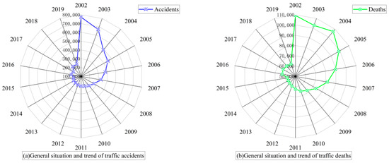
Figure 1.
General situation and trend of traffic accidents and deaths by provinces of China from 2002 to 2019.
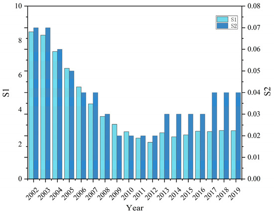
Figure 2.
Mortality rate of 100 million passenger turnover and 10,000 passenger volume in all provinces of China from 2002 to 2019.
From the perspective of time distribution, as shown in Table 2 and Figure 1, the number of traffic accidents and deaths have a gradual decline during 2002–2013, with a slight increase after 2015; however, a downward trend is observable on the whole. The maximum number of traffic accidents in 2002 is 1.89 times the minimum in 2013. Meanwhile, the maximum number of traffic deaths in 2002 is 4.12 times the minimum in 2014, which shows that the traffic safety situation tends to be stable and better, and the traffic safety work in China has achieved fruitful results.
Figure 2 shows that the annual passenger turnover per 100 million person kilometers and average accident mortality per 10,000 person kilometers in China had a steady descending trend from 2002 to 2012 and increased slightly from 2012 to 2019; however, the overall state of affairs tended to be stable. In detail, the values from 8.51 people per 100 million person kilometers and 0.07 people per 10,000 person kilometers in 2002 to 2.12 people per 100 million person kilometers and 0.02 people per 10,000 person kilometers in 2013, mean that the cost of transportation accidents in China has been significantly reduced, and the macro situation of traffic safety has been significantly improved.
From the perspective of spatial distribution, due to the expansive land area of China and the great differences in the topography, geology, and economic development of various regions, the traffic safety conditions of various regions are conspicuously different (Li et al., 2021). Additionally, Figure 3 indicates that the geographical distribution of traffic accidents and deaths is presented in various colors, which were divided into five levels. The darker the color of an area, the more traffic accidents or deaths there are in that area. Generally speaking, the southern provinces (e.g., Guizhou, Sichuan, and Guangdong) have more traffic accidents and deaths than the northern provinces (e.g., Gansu, Nei Monggol, and Shanxi). Furthermore, this difference also exists between the eastern coastal provinces (e.g., Zhejiang, Jiangsu, and Shandong) and the northwest provinces (e.g., Qinghai, Xinjiang, and Tibet).
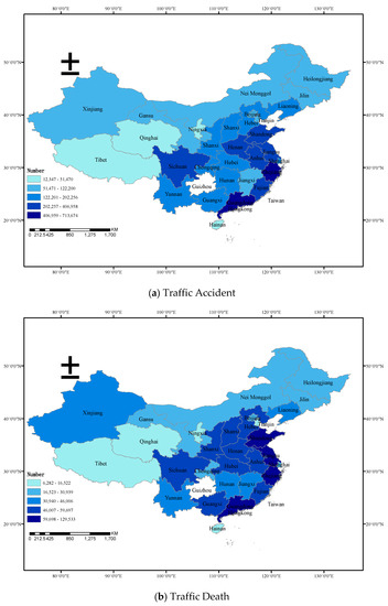
Figure 3.
Spatial distribution of traffic accidents (a) and deaths (b) by provinces of China from 2002 to 2019.
3.2. Global Spatial Autocorrelation of Traffic Accidents
We calculated the spatial autocorrelation of traffic accidents in various provinces of China from two aspects: one is the data of traffic accidents, and the other is the data of deaths caused by traffic accidents. Then, the results were arranged in Table 3 and Table 4.
Table 3.
Moran’s Index of traffic accidents from 2002 to 2019.
Table 4.
Moran’s Index of the death of traffic accidents from 2002 to 2019.
Table 3 and Table 4 suggest that, except for the data of traffic accidents in 2008–2010 and 2017, the data of traffic deaths in 2014–2017 failed to pass the 90% confidence test. All other years passed the 90% confidence test. There is a significant positive spatial autocorrelation in the occurrence of traffic accidents. In detail, its spatial autocorrelation characteristics signify that the provinces with a close number of traffic accidents and deaths show spatial aggregation; that is, the provinces with a higher number of traffic accidents and deaths also have a higher number of accidents and deaths in their adjacent provinces. On the contrary, in the provinces with a lower number of traffic accidents and deaths, the number of traffic accidents and deaths in neighboring provinces is also low.
To further excavate the spatial autocorrelation characteristics of provinces, we discussed the Moran I index of traffic accidents and deaths in 2002–2019 based on the coordinate axis (Figure 4), where gray are the years when the confidence test failed.
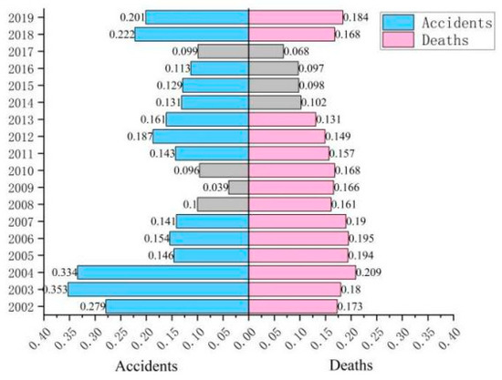
Figure 4.
Change chart of Moran’s I index of the number of traffic accidents and deaths in various provinces of China from 2002 to 2019.
As can be seen from Figure 4, with the passage of time, the Moran I index of the data of traffic accidents and deaths in China showed a downward trend from 2002 to 2019, but it showed a short upward trend from 2017 to 2018. It is worth noting that the Moran I index of accidents dropped from the highest of 0.3530 to the lowest of 0.1130, and the Moran index of deaths toll dropped from the highest of 0.2090 to the lowest of 0.1310, which shows that the trend of spatial autocorrelation in this period is weakening, and the spatial aggregation of traffic accidents and deaths in neighboring provinces is weakening.
3.3. Local Spatial Autocorrelation of Traffic Accidents
The above calculation of the global Moran I index shows that there is global autocorrelation, which indicates that the traffic accidents and deaths in China’s provinces have an aggregation effect; however, this statistic cannot show the spatial autocorrelation of local space. Therefore, we need to use the Moran scatter plot and the LISA map for further study.
3.3.1. Local Spatial Autocorrelation of Traffic Accidents Based on Moran Scatter Chart
We use the average sampling method to select four years for research in order to investigate the heterogeneity of local spatial units and ensure that the research conclusion can represent the overall situation from 2002 to 2019. In addition, the selected data are the years that passed the confidence test in Table 3 and Table 4. Finally, we selected the traffic accident and death data in 2002, 2007, 2013, and 2019, and studied the Moran scatter plot, with each dot representing a province and city. The results are shown in Figure 5 and Figure 6.
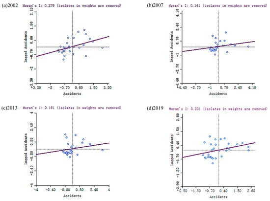
Figure 5.
Moran scatter chart of the number of traffic accidents in various provinces of China in (a) 2002, (b) 2007, (c) 2013 and (d) 2019.
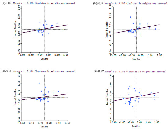
Figure 6.
Moran scatter chart of the number of traffic deaths in various provinces of China in (a) 2002, (b) 2007, (c) 2013 and (d) 2019.
As is evident from Figure 5 and Figure 6, some provinces are far from other provinces, which are mainly located in the first and second quadrants. Moreover, the data of traffic accidents and deaths in 2019 are relatively scattered, and the distribution in other years is relatively concentrated, mainly in the third quadrant. These faraway provinces far from other provinces are mainly located in the eastern coastal areas, which are areas of rapid economic development and dense population, and the data of traffic accidents and deaths are much higher than in other provinces and cities in China. Those that play a momentous role have a great influence on the global spatial autocorrelation of the data of traffic accidents and deaths. In addition, the data of traffic accidents in Tibet and Qinghai are much lower than the national average, which also has a certain impact on the spatial autocorrelation of the overall data of traffic accidents and deaths.
As shown in Table 5 and Table 6, the provinces correspond to Moran scatter plots of provincial traffic accidents and deaths in China in 2002, 2007, 2013, and 2019, which reveals that the vast majority of provinces are located in the first and third quadrants, which belong to the molds of high–high gather and low–low gather. Among them, the provinces of the low–low aggregation type are more numerous than those of the high–high aggregation type.
Table 5.
Moran scatter chart of the number of provincial traffic accidents in 2002, 2007, 2013 and 2019.
Table 6.
Moran scatter chart of the number of provincial traffic deaths in 2002, 2007, 2013 and 2019.
Firstly, the provinces surrounded by high values in these four years (located in the first quadrant) are Jiangsu, Anhui, and Fujian. In recent years, the above provinces and their adjacent provinces have experienced a high data of traffic accidents and deaths, which is unusual for a relatively developed part of China’s economy. Moreover, about 15 provinces or cities are in the third quadrant, that is, they are low-value provinces or cities surrounded by low-value provinces, which receive attention in western China and a few eastern regions (Beijing and Tianjin). The data of traffic accidents and deaths in these provinces or cities are markedly lower than the national average. At the same time, most of these provinces or regions are economically underdeveloped areas in China. Provinces or regions falling into the first and third quadrants have a strong spatial positive correlation, that is, homogeneity.
Furthermore, Jiangxi is the high-value province surrounded by low-value provinces in these four years (located in the second quadrant), while Guangxi, which is surrounded by high-value provinces in 2019, is surrounded by high-value regions in the other three years, indicating that the data of traffic accidents and deaths in Guangxi are lower than that of surrounding provinces. The data of traffic accidents and deaths in Guangxi in 2019 tend to be consistent with those in the neighboring provinces over time, forming a type of high–high aggregation. Moreover, Sichuan is the province with the highest values surrounded by low-value provinces in these four years (located in the fourth quadrant), implying that the data of traffic accidents and deaths in neighboring provinces and cities in Sichuan is low, and Sichuan is the province with more serious traffic accidents in the corresponding region. Overall, provinces and regions in the second and fourth quadrants have a strong spatial negative correlation, suggesting heterogeneity.
Generally speaking, the data of traffic accidents and deaths in China fall roughly into two quadrants: high–high and low–low, with little inter-annual variation, revealing that there has been a perceptible spatial dual structure in the regional difference in the data of traffic accidents in China since 2002. The vast bulk of traffic accidents occur in economically developed areas of the southeast coast. At the same time, it demonstrates that traffic accident control should be tailored to local conditions and that the geographical space cannot be ignored. Different measures, as well as standard measures, must be used for different regions.
3.3.2. Local Spatial Autocorrelation of Traffic Accidents Based on LISA Map
In order to further explore the spatial autocorrelation between local provinces, we also need to use the LISA map for research. Figure 7 and Figure 8 show the provincial local spatial autocorrelation LISA map of the data of traffic accidents and deaths in various provinces and cities in China. Different colors correspond to different aggregation types; blue corresponds to low–low aggregation, red represents high–high aggregation, purple means low–high aggregation, and pink corresponds to high–low aggregation.
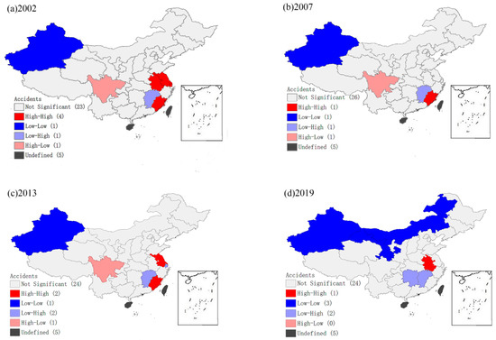
Figure 7.
LISA plots of the number of traffic accidents in various provinces of China in (a) 2002, (b) 2007, (c) 2013 and (d) 2019.
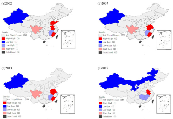
Figure 8.
LISA plots of the number of traffic deaths in various provinces of China in (a) 2002, (b) 2007, (c) 2013 and (d) 2019.
As shown in Figure 7, in terms of the data of traffic accidents in 2002, the provinces with significant positive spatial autocorrelation are Fujian, Anhui, and Jiangsu, while the province with negative spatial autocorrelation is Xinjiang. In 2007, a slight change in the positive spatial autocorrelation province occurred, but it is still located in the southeast coastal area (Fujian), and the negative spatial autocorrelation area did not change. In 2013, the provinces with significant positive spatial autocorrelation increased compared with 2007, including Jiangsu, which is also located in the southeast coastal area. The situation in 2019 is very different from that in other years. Specifically, Anhui is the only province with a significant positive spatial autocorrelation, while the province with significant negative spatial autocorrelation has expanded from Xinjiang to Inner Mongolia and Gansu. It is worth noting that, except in 2019, the province with high–low concentration has always been Sichuan.
Similarly, as indicated in Figure 8, it can be found that the data of traffic deaths are roughly the same as the data of accidents, with only a slight difference. That is, in 2002, in terms of traffic fatalities, the provinces with positive spatial autocorrelation were Fujian, Anhui, Shandong, and Xinjiang, all in negative spatial autocorrelation; In 2007, the provinces with significant positive spatial autocorrelation changed slightly, but they are located in the southeast coastal areas (Fujian, Anhui, and Jiangsu), and the regions with significant negative spatial autocorrelation did not change. Provinces with significant positive and negative spatial autocorrelation are the same in 2013 as they were in 2007. Moreover, the data of traffic deaths in 2019 are the same as the data of traffic accidents mentioned above. Similarly, except for 2019, Sichuan has been showing high-low aggregation.
As mentioned above, it is not difficult to identify the reasons.
Firstly, it is located in the southeast coastal areas like Fujian, Jiangsu, and Zhejiang, which are characterized by a high level of urbanization and industrialization that far exceeds that of many inland cities. As a result, these cities have a developed economy, a large resident population, and a traffic network extending in all directions, which makes these cities show extremely significant high-value aggregation characteristics, namely a positive radiation effect.
Secondly, Xinjiang, located on the northwest border of China, has always been a significant low–low agglomeration, which indicates that the traffic safety in Xinjiang and its surrounding provinces has always been good. The main reasons are that the economic and social development in Xinjiang and its surrounding provinces has been relatively slow, and in addition, due to the restrictions on ethnic minorities, historical and geographical conditions, small resident population, and inconvenient transportation, the traffic development in Xinjiang and its surrounding provinces has lagged behind for a long time. In addition, the reason that Gansu and Nei Monggol in 2019 show a negative spatial autocorrelation is that traffic safety rectification actions have been carried out in recent years.
Thirdly, Sichuan has always been a province of high–low aggregation, except for in 2019. Due to the complex and diverse geographical terrain and poor road conditions in Sichuan, the traffic safety situation in Sichuan is severe. However, since December 2013, road traffic safety rectification has been carried out in Sichuan; with the unremitting efforts of the public security traffic management department, the road traffic safety form in Sichuan has continued to improve (Sichuan Daily, 26 November 2015). In other words, this is the reason why the phenomenon of high–low aggregation disappeared in 2019.
3.4. Significance of Research
This paper explores the spatial autocorrelation characteristics and spatial heterogeneity among neighboring provinces or cities, reveals the spatial and temporal distribution characteristics of road traffic accidents in China, has positive significance for deepening the risk cognition of road traffic accidents, and can provide a theoretical basis for the government to formulate regional traffic management policies, construct corresponding control policies, and allocate traffic control resources.
4. Conclusions
Taking the traffic accident data of 31 provinces in China from 2002 to 2019 as an example, the purpose of this study is to investigate the traffic accident data in China’s traffic management department and explore the spatio-temporal distribution pattern. It draws the following conclusions.
The data on traffic accidents and deaths in various provinces in China are not completely random in spatial distribution but have significant global spatial autocorrelation and local spatial autocorrelation. Specifically, areas with high traffic accidents and fatalities are adjacent to areas with higher traffic accidents and fatalities, while areas with lower traffic accidents and fatalities are adjacent to areas with lower traffic accidents and fatalities. Moreover, this situation has gradually increased in recent years.
There is spatial autocorrelation and heterogeneity in the data of traffic accidents and deaths in China. Concretely, the areas with high traffic accidents are mainly concentrated in the economically developed eastern coastal areas, and the areas with low traffic accidents are mainly concentrated in the economically underdeveloped areas of the northwest region. In addition, the research also found that in the atypical areas of traffic accidents, that is, the areas deviating from the overall positive spatial autocorrelation trend, the data of traffic accidents and deaths is higher in more developed provinces such as Jiangsu, Anhui, Fujian, and Shandong are higher; moreover, the number of traffic accidents and deaths in Sichuan is significantly higher than those in neighboring provinces and cities, but this phenomenon has disappeared in recent years.
Additionally, the following characteristics can be seen from the data of traffic accidents and deaths in China’s provinces: one is the significant global spatial aggregation effect, where the provinces with high-value aggregation have gradually expanded from the southeast coastal areas to a few southwest areas, and the provinces with low-value aggregation are generally stable, mainly concentrated in the western region; the other is that the local spatial autocorrelation is obvious, and the provinces with positive spatial autocorrelation tend to be stable in the early stage, and gradually expand from Xinjiang to Gansu and Nei Monggol in the later stage.
Furthermore, the causes of regional agglomeration and spatial heterogeneity of traffic accidents and deaths in China are not only affected by geography and topography but also related to the level of economic development. Consequently, relevant departments can adjust measures to local conditions and treat them differently when formulating traffic control policies and formulating corresponding policies for traffic accidents in different regions to better improve traffic safety.
Based on the spatial statistical method, this paper analyzes the number of traffic accidents and deaths in China’s provinces and studies the spatial autocorrelation characteristics and spatial heterogeneity between neighboring provinces or cities. The research conclusion can provide a scientific basis for traffic safety management and control between neighboring provinces or cities.
Considering that the number and consequences of traffic accidents are closely related to the number of motor vehicles, we will collect relevant data for further research in the follow-up study.
Funding
This research was funded by National Natural Science Foundation of China (No. 52179136).
Conflicts of Interest
The authors declare that they have no known competing financial interests or personal relationships that could have appeared to influence the work reported in this paper.
References
- World Health Organization. World Report on Road Traffic Injury Prevention; WHO: Geneva, Switzerland, 2021. [Google Scholar]
- Singh, S.K. Road traffic accidents in India: Issues and challenges. Transp. Res. Proced. 2017, 25, 4708–4719. [Google Scholar] [CrossRef]
- Alam, M.S.; Mahumd, S.M.; Hoque, M.S. Road accident trends in Bangladesh: A comprehensive study. In Proceedings of the 4th Annual Paper Meet, and 1st Civil Engineering Congress, Dhaka, Bangladesh, 22–24 December 2011; pp. 172–180. [Google Scholar]
- PPRC. PPRC Final Report 2014. In Road Safety in Bangladesh Ground Realities and Action Imperatives; Power and Participation Research Center BRAC: Dhaka, Bangladesh, 2014. [Google Scholar]
- WHO. Global Health Estimatea: Deaths by Cause, Age, Sex, and Country, 2000–2012; WHO: Geneva, Switzerland, 2014; p. 9. [Google Scholar]
- World Health Organization. Global Status Report on Road Safety 2018 [EB/OL]; WHO: Geneva, Switzerland, 2018. [Google Scholar]
- Wang, D.Y.; Liu, Q.Y.; Ma, L. Road traffic accident severity analysis: A census-based study in China. J. Saf. Res. 2019, 70, 135–147. [Google Scholar] [CrossRef] [PubMed]
- Yang, Z.K.; Zhang, W.P.; Feng, J. Predicting multiples of traffic accident severity with explanations: A multi-task deep learning framework. Saf. Sci. 2022, 146, 105522. [Google Scholar] [CrossRef]
- Ma, Z.J.; Mei, G.; Salvatore, C. An analytic framework using deep learning for prediction of traffic accident injury severity based on contributing factors. Accident Anal. Pred. 2021, 160, 106322. [Google Scholar] [CrossRef] [PubMed]
- Sun, L.L.; Liu, D.; Chen, T.; Zhao, H. Analysis on the accident casualties influenced by several economic factors based on the traffic-related data in China from 2004–2016. Chin. J. Traumatol. 2019, 22, 75–79. [Google Scholar] [CrossRef]
- Smeed, R.J. The usefulness of formulate in traffic engineering and road safety. Accident Anal. Prev. 1972, 4, 303–312. [Google Scholar] [CrossRef]
- Zhao, L.; Xu, H.K. Traffic accident prediction based on gray weighted Markov SCGM (1,1) c. Com. Eng. Appl. 2012, 48, 11–15. [Google Scholar]
- Mannering, F.L.; Shankar, V.; Bhat, C.R. Unobserved heterogeneity and the statistical analysis of highway accident data. Anal. Methods Accid. Res. 2016, 11, 1–16. [Google Scholar] [CrossRef]
- Liu, C.; Sharma, A. Using the multivariate spatio-temporal Bayesian model to analyze traffic crashes by severity. Anal. Methods Accid. Res. 2018, 17, 14–31. [Google Scholar] [CrossRef]
- Le, K.G.; Liu, P.; Lin, L.T. Determining the road traffic accident hotspots using GIS-based temporal-spatial statistical analytic techniques in Hanoi, Vietnam. J. Geos. Inf. Sci. 2020, 23, 12. [Google Scholar] [CrossRef]
- Wee, C.; He, X.; Win, W.; Ong, M. Geospatial analysis of severe road traffic accidents in Singapore in 2013–2014. Sin. Med. J. 2020, 62, 353. [Google Scholar] [CrossRef]
- Dereli, M.A.; Erdogan, S. A new model for determining the traffic accident black spots using GIS-aided spatial statistical methods. Transp. Res. Part A Pol. Prac. 2017, 103, 106–117. [Google Scholar] [CrossRef]
- Satria, R.; Castro, R. GIS tools for analyzing accidents and road design: A review. Transp Res Proced. 2016, 18, 242–247. [Google Scholar] [CrossRef]
- Lu, H.P.; Luo, S.X.; Li, R.M. Study on spatial distribution characteristics of road traffic accidents in Shenzhen based on GIS analysis. Chin. J. Hig. 2019, 32, 156–164. [Google Scholar]
- McFadden, D.L. Chapter 24 Econometric analysis of qualitative response models. In Handbook of Econometrics; North-Holland Publishing Company: Amsterdam, The Netherlands, 1984; Volume 2, pp. 1395–1457. [Google Scholar]
- Bhat, C.R.; Astroza, S.; Hamdi, A.S. A spatial generalized ordered-response model with skew normal kernel error terms with an application to bicycling frequency. Tran. Res. Part B Met. 2017, 95, 126–148. [Google Scholar] [CrossRef]
- Fernández, D.; McMillan, L.; Arnold, R.; Spiess, M.; Liu, I. Goodness-of-fit and generalized estimating equation methods for ordinal responses based on the stereotype model. Stats 2022, 5, 30. [Google Scholar] [CrossRef]
- Wang, H.J.; Liu, Y.M.; Zhang, B.; Xu, S.; Jia, K.J.; Hong, S. Driving force analysis of urban land expansion in Wuhan City Circle Based on logistic gtwr model. J. Agric. Eng. 2018, 34, 248–257, 310. [Google Scholar]
- Valencia, C.; Ramírez, A. Spatio-temporal correlation study of traffic accidents with fatalities and injuries in Bogota (Colombia). Accid. Anal. Prev. 2020, 149, 105848. [Google Scholar]
- Li, J.; Zeng, X.S.; Sun, L.; Liu, W.; Li, P. Study on the Evolution of Spatial and Temporal Layout of Road Traffic Safety Level in China. Chin. J. Saf. Sci. 2021, 31, 136–143. [Google Scholar]
- Zheng, Y.P.; Feng, C.G.; Jing, G.X.; Qian, X.M.; Li, X.J.; Liu, Z.Y.; Huang, P. A statistical analysis of coal mine accidents caused by coal dust explosions in China. J. Loss Prev. Proc. Ind. 2009, 22, 528–532. [Google Scholar] [CrossRef]
- Garten, R.J.; Davis, C.T.; Russell, C.A. Antigenic and genetic characteristics of swine- origin 2009 A (H1N1) influenza viruses circulating in humans. Science 2009, 325, 197. [Google Scholar] [CrossRef] [PubMed]
- Ma, Q.; Jia, P.; Sun, C.; Kuang, H. Dynamic evolution trend of comprehensive transportation green efficiency in China:From a spatio-temporal interaction perspective. J. Geog. Sci. 2022, 32, 477–498. [Google Scholar] [CrossRef]
- Yin, J.; Li, S.; Zhou, L.; Jiang, L.; Ma, W. Spatial heterogeneity of the economic growth pattern and influencing factors in formerly destitute areas of China. J. Geog. Sci. 2022, 32, 829–852. [Google Scholar] [CrossRef]
- Moran, P.A.P. Notes on continuous stochastic phenomena. Biometrika 1950, 37, 17–23. [Google Scholar] [CrossRef]
- Long, T.T.; Somenahalli, S. Using GIS to Identify Pedestrian-Vehicle Crash Hot Spots and Unsafe Bus Stops. J. Pub. Transp. 2011, 14, 6. [Google Scholar]
- Yang, S.Q.; Xing, Q.Y.; Dong, W.H.; Li, S.P.; Zhan, Z.C.; Wang, Q.Y.; Yang, P.; Zhang, Y. Temporal and spatial response of target factors of influenza A (H1N1) in Beijing. J. Geog. 2018, 35, 2139–2152. [Google Scholar]
- Zhao, X.C. Review and analysis of road traffic accidents in Chongqing. High. Tran. Tec. 2003, 2, 117–119, 123. [Google Scholar]
- Xu, R.T.; Lu, J. Analysis of traffic accident data in Jiangsu Province. Chin. J. Saf. Sci. 2007, 17, 11–15. [Google Scholar]
- Wang, H.M. Analysis on the current situation and characteristics of highway traffic accidents in China. Chin. J. Saf. Sci. 2009, 19, 121–126, 179. [Google Scholar]


Publisher’s Note: MDPI stays neutral with regard to jurisdictional claims in published maps and institutional affiliations. |
© 2022 by the authors. Licensee MDPI, Basel, Switzerland. This article is an open access article distributed under the terms and conditions of the Creative Commons Attribution (CC BY) license (https://creativecommons.org/licenses/by/4.0/).