Water Quality Variation Law and Prediction Method of a Small Reservoir in China

Abstract

Compared with the attention of large reservoirs, the water quality of small reservoirs also needs attention. In recent years, the problem of reservoir water quality has become increasingly serious. How to predict reservoir water quality may be an urgent problem to be solved. Taking the Yangmeiling reservoir as an example, this paper collects the hydrological and water quality data of the Yangmeiling reservoir in the last ten years, analyzes the relationship between hydrological and water quality data, and uses a machine learning method to simulate the relationship between water quality and hydrological data. The results show that the water quality of small reservoirs can be simply linked with hydrological data and can be predicted through hydrological data, and has high simulation accuracy. This method can be popularized in the simulation and prediction of the water quality of small reservoirs; it does not provide a theoretical basis for the water quality management of small reservoirs.

1. Introduction

Reservoirs are important water collection and storage measures for human beings, and most of them carry the functions of living, production, flood protection, water supply and power generation [1,2]. Because reservoirs often supply water to cities and farmland, their water quality is often the focus of our attention. As the main indicators of reservoir water quality evaluation, the concentration of nitrogen and phosphorus is often the most concerning. Excessive nitrogen and phosphorus will not only affect the water quality but also cause eutrophication of the water body [3,4,5]. The cyanobacteria will produce harmful substances, affecting the safety of people and crops.

Eutrophication of aquatic ecosystems refers to an ecological state in which the biological process driven by the increase in nutrient load in the basin leads to the proliferation of primary producers (phytoplankton, hydrophytes and cyanobacteria), hypoxia and the loss of biodiversity. Excessive total phosphorus (TP) is one of the main factors leading to eutrophication and algal blooms in rivers, lakes and reservoirs. In view of the close relationship between TP and total nitrogen (TN) concentrations and algal biomass, TP and TN can be used as indicators of eutrophication to estimate phytoplankton concentrations. If TP in the reservoir can reach a high level under strong wind or other conditions, it will not meet the irrigation and drinking water supply standards [6]. The research on the influence of nitrogen and phosphorus content in lakes and reservoirs mainly focuses on the input of exogenous pollutants and the release of endogenous pollutants. Exogenous pollutants mainly include the nitrogen and phosphorus content contained in the incoming flow of lakes and reservoirs [7]. Endogenous phosphorus and nitrogen are usually released into lakes through the diffusion process or after the sediment is disturbed [8]. For some shallow lakes, the impact of wind speed on lake hydrodynamic forces can promote the disturbance of sediment and release nitrogen and phosphorus [9,10]. Many articles also focus on the impact of temperature on the concentration of nitrogen and phosphorus in lakes and reservoirs. The temperature will affect the biological activity in lakes and reservoirs, and thus affect the absorption and release of nitrogen and phosphorus [11,12].

The prediction of nitrogen and phosphorus concentration is conducive to the optimization of reservoir management systems. In order to simulate and predict the changes in nitrogen and phosphorus concentration in lakes and reservoirs, many scholars have carried out indoor and outdoor experiments. Bai et al. [13] determined the release law of TP in lakes under the influence of hydrodynamic forces through indoor experiments and used the lattice Boltzmann model to simulate and predict the TP concentration change. Wells and Berger [14] established the response model of dissolved oxygen in Spokane lake to phosphorus load. Katsev [15] studied the time scale of the response of lakes to the external input of restrictive nutrients (such as phosphorus), considered the nutrient cycle in sediments, and simulated and predicted it through a simple mass balance model. Yang et al. [16] used land use data, precipitation data, digital elevation model (DEM) data and the ecosystem services integrated assessment and trade-off (invest) model to simulate the nitrogen and phosphorus output of Bosten Lake Basin. Du et al. [17] obtained 216 sample points, 172 modeling points and 44 verification points from five field experiments in Taihu Lake and established a semi-analytical model for estimating TP concentration based on the absorption coefficient, which has high simulation accuracy. Han et al. [18] studied systematic nitrogen transformation in tropical freshwater systems using a three-dimensional water eutrophication model, which simulates hydrodynamics, phytoplankton processes, and nutrient cycling in Delft3D. At the same time, machine learning has also been applied to the prediction of lake water quality, because machine learning has many advantages [19]. Bai et al. [20] collected a large number of lake monitoring data based on data and machines and used natural selection based machine learning technology genetic programming to search for the robust relationship between phosphorus concentration, wind speed and water temperature. Sriworamas et al. [21] established the model of abundant water and insufficient water suitable for small reservoirs by comparing different optimization methods.

To sum up, there are many prediction models for lake water quality, most of which are based on the changes in the water quality of lakes and reservoirs; the models for simultaneous measurement with the upstream incoming water are rare. The model is often accompanied by complex reaction formulas, which makes the operation speed very slow. This operation speed often cannot meet the real-time management of water quality control in lakes and reservoirs. In addition, most of the studies prefer to study the prediction of nitrogen and phosphorus in large lakes and reservoirs; it is also necessary to study the prediction of nitrogen and phosphorus in small reservoirs. Based on the monitoring data of lakes and upstream water for ten years, the aims of this paper are to find the relationship between the data and establish a fast model for lake water quality prediction based on a machine learning method, which provides a basis for rapid response to the numerical situation of lakes and provides a theoretical basis for lake water quality control.

2. Study Methods

2.1. Study Area

The study area is located in Ninghai County, Ningbo City, Zhejiang Province, China, between 29°06′~29°32′ N and 121°09′~121°49′ E (Figure 1). It belongs to the subtropical monsoon humid climate area. It is dominated by east and south winds all year round. The climate is warm and humid, with four distinct seasons, abundant sunshine and rain. The annual average air temperature is 15.3~17 °C, the annual sunshine is about 1900 h, the average relative humidity is 78%, and the annual average precipitation is 1000~1600 mm. The average residence time is 12 days and residence time at peak flow is 3 days. The average depth of the Yangmeiling reservoir is 5 m, and the reservoir area is 1.12 × 10⁶ m². The max depth is 8 m, and so far, there is no algal bloom phenomenon. The volume of the reservoir is 5.6 × 10⁶ m³, and it is a typical small reservoir that takes into account both urban water supply and farmland water supply.

2.2. Data Analysis

Data collection is from 2012 to 2021 in the past decade. The collection of hydrological data mainly includes monthly average rainfall, monthly average wind speed, monthly average temperature, monthly average evaporation and monthly average runoff. The data are from the Hongjiata monitoring station. Water quality data mainly include TN and TP. The data come from the Hongjiata monitoring station and the Yangmeiling monitoring station. Three samples with a volume of 500 mL were taken at the depth of 1 m, 2 m and 3 m at each site by water sampler. The samples were taken every day and adopted the monthly average value. TP in the water was ascertained using the molybdenum antimony spectrophotometry method. TN was determined by ultraviolet spectrophotometry using the alkaline potassium persulfate digestion method. It is difficult to establish the relationship between rainfall, water quality and flow if the daily data are used for simulation as there is not rainfall every day. Many studies are based on the monthly average data [22,23,24,25,26,27,28,29,30], which prove that the monthly average data play a representative role in displaying the water quality of reservoirs and lakes. Therefore, this paper adopts the monthly average data.

Statistical methods were applied to process the analytical data in terms of the distribution and correlation among the studied parameters. Statistical analysis was carried out using the SPSS 16 statistical package. Pearson correlation coefficient was used in the correlation analysis of the data, and the probability P was 0.05 and 0.01, respectively.

2.3. Machine Learning Model–Eureqa

The previous data solution method first assumes a mathematical formula structure and then uses the multi-objective regression method or trial and error method to find the optimal parameters. Some studies have tried to use programs to find the optimal mathematical formula structure without giving an empirical model in advance [30,31]. Schmidt and Lipson [32] found that machine learning (ML) technology can find the relationship between variables without giving the relationship between data. The method of the genetic program has now become a very effective method to find the relationship between data, not just a purely statistical and numerical model. This method has found in practice that genetic programs can find satisfactory solutions in complex systems. These successful examples have prompted the authors to study the water quality prediction of reservoirs.

A genetic program regards the sub-formula of the formula as an individual in the evolutionary population. The data need to be divided into three groups: the training group will produce sub-expressions generation after generation, the verification group will choose the best sub-expressions, and then eliminate the sub-expressions that perform poorly; the test group will be used to test the quality of the results [33]. Elimination, crossover, and random mutation occur in the process of evolution. Genetic programs obtain meaningful connections between data in the process of evolution. Genetic programs produce a set of expressions with different complexity, but the program will give priority to expressions that are neither complex nor too simple. An overly simple expression will be inaccurate, but an overly complex expression will be too adaptive. When selecting an expression, we need to comprehensively consider the accuracy and complexity of the formula [34]. Here, we use Eureqa [35] which is a method that can be effectively applied in the prediction of the formula (https://www.nutonian.com/download/eureqa-onprem-download/ (accessed on 21 January 2017).

2.4. Data Prediction

We divided the data into three groups: four years of data are used for training, three years of data for validation and three years of data for testing. The formula is obtained by considering the accuracy and complexity. The independent variable and dependent variable of the simulation should be treated as dimensionless, which is mainly manifested in the treatment of the measured maximum value with the measured value, as shown in Equation (6). The coefficient of determination (R²) and mean absolute error (MAE) were adopted to judge the simulation result, and the MAE and R² were determined by:

$$R^2=1-\frac{SSE}{SST}$$

(1)

$$SST={{\displaystyle \sum }}_{i=1}^N{\left(Y_i-meanY\right)}^2$$

(2)

$$SSE={{\displaystyle \sum }}_{i=1}^N{\left(Y_i-X_i\right)}^2$$

(3)

$$meanY=\frac{1}{N}{{\displaystyle \sum }}_{i=1}^N{Y}_i$$

(4)

$$MAE=\frac{{{\displaystyle \sum }}_1^N\left|Y_i-X_i\right|}{N}$$

(5)

$$\frac{y}{y_{max}}=f\left(\frac{x_1}{x_{1max}},\frac{x_2}{x_{2max}},\dots \frac{x_i}{x_{imax}}\right)$$

(6)

where $N$ denotes the number of lateral measuring points; $X$ and $Y$ represent the calculated and measured values, respectively, $SSE$ is the Sum of Squares for Error, and $SST$ is the Sum of Squares for total. $y$ is the dependent variable, and $y_{max}$ is the max measured value of the dependent variable; $x_i$ is the ith independent variable, and $x_{imax}$ is the max measured value of the independent variable.

Eureqa’s main steps are:

(1)

Enter training and validation data.

(2)

The random equation generator generates preliminary equations that combine operational factors (such as constants and variables) with operations (addition, subtraction, multiplication, division, etc.).

(3)

MAE was used to compare the predicted values generated by the equations with the measured values of the test group. Bad solutions are discarded. The rest of the program hybridizes with the probability function given by the program and generates a new sub-expression according to the inherent mutation probability function.

(4)

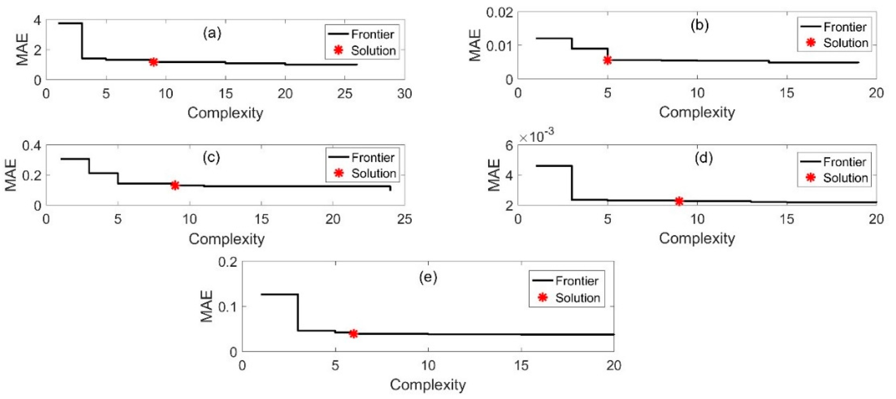
Stop the program when a reasonable solution appears (it will not stop automatically). This program will provide a series of solutions with different accuracy and complexity.

3. Results

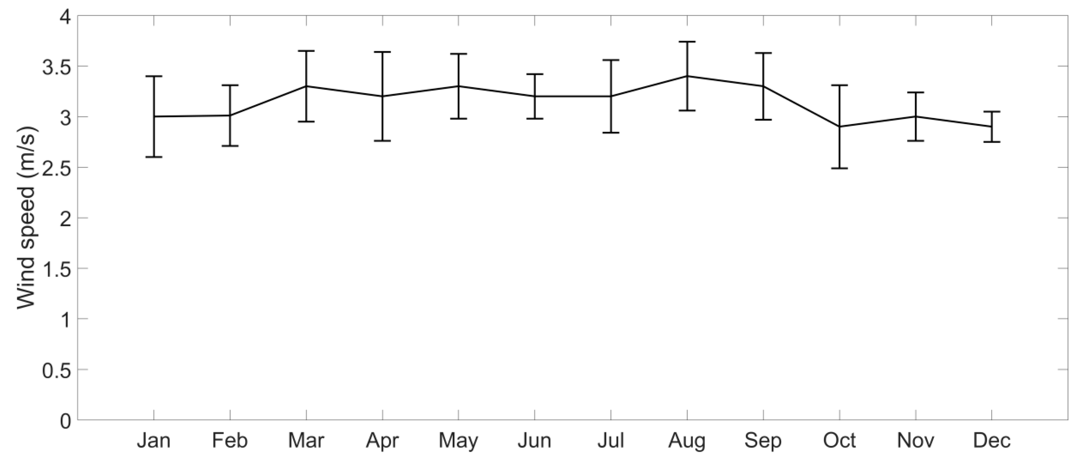
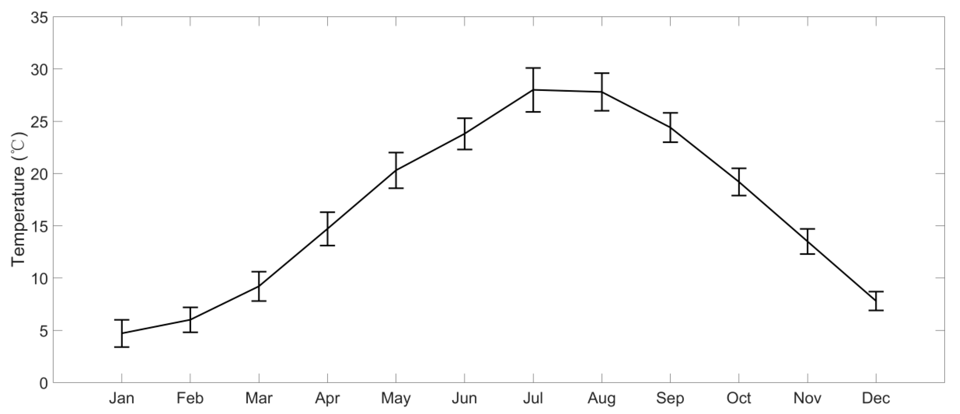
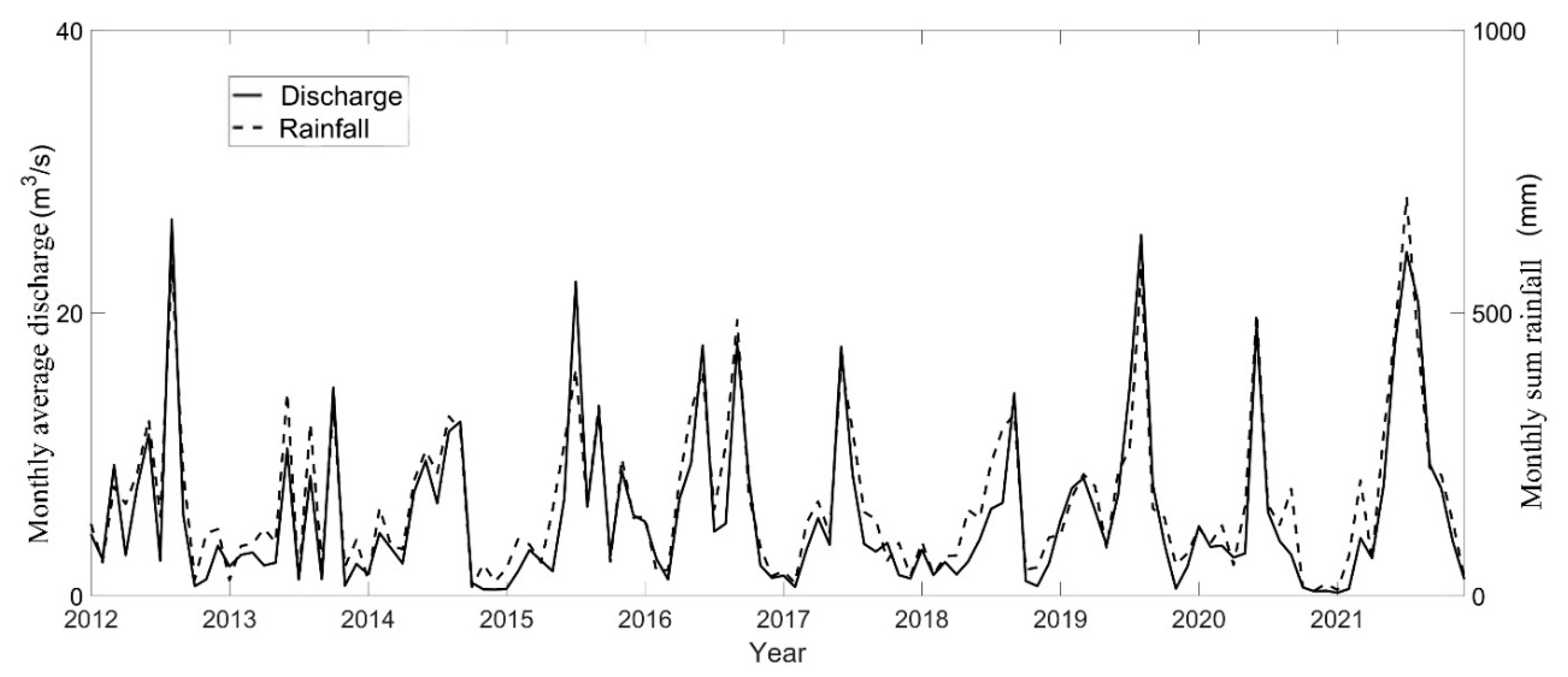
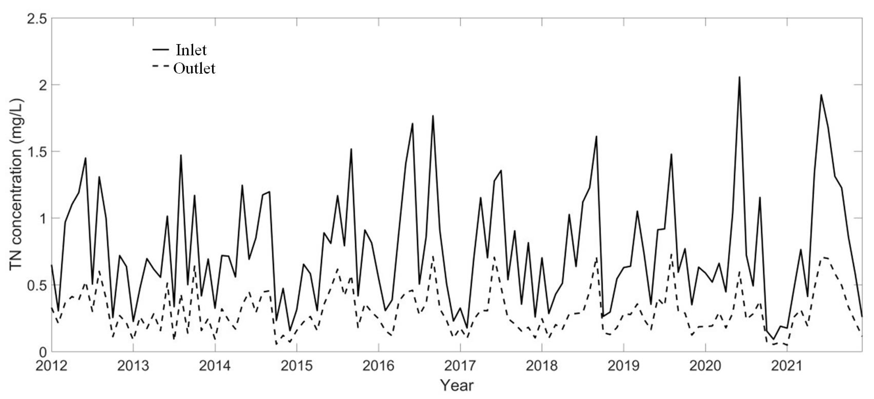
3.1. Vary Law of the Parameters in Yangmeiling Reservoir

The monthly average wind speed in the study area in the last ten years is shown in Figure 2. The average wind speed is between 2.9~3.4 m/s, and the wind speed changes relatively evenly throughout the year. The monthly average air temperature ranged between 4.7 and 28 °C and changed relatively evenly throughout the year in the study area in the last ten years (Figure 3).

The data of the river’s monthly average discharge and the basin’s monthly average rainfall are shown in Figure 4. It can be seen that the discharge increases with the increase in rainfall and decreases with the decrease in rainfall. The river discharge varies from 0.2 to 26.6 m³/s, and the rainfall varies from 8.5 to 705.5 mm. Rainfall and discharge are higher in the middle of the year and are relatively small at the beginning and end of the year. The TP concentration of the Inlet monitoring station varies from 0.007 to 0.075 mg/L, and that of the Inside monitoring station varies from 0.003 to 0.031 mg/L shown in Figure 5. The TP concentration of the water flow at the inlet of the reservoir is significantly higher than that in the reservoir, and the concentration change law is close to that in the middle of the year. The concentration is large, and the concentration at the beginning and end of the year is relatively small. The TP concentration of the Inlet monitoring station varies from 0.091 to 2.056 mg/L, and the TN concentration of the Inside monitoring station varies from 0.048 to 0.726 mg/L shown in Figure 6. The TN concentration of the water at the inlet of the reservoir is significantly higher than that in the reservoir. The concentration is large, and the concentration at the beginning and end of the year is relatively small. The correlation coefficients between various parameters are shown in

Table 1. The correlation between different parameters.

	$\mathit{T}{\mathit{P}}_{\mathit{i}\mathit{n}\mathit{l}\mathit{e}\mathit{t}}$	$\mathit{T}{\mathit{N}}_{\mathit{i}\mathit{n}\mathit{l}\mathit{e}\mathit{t}}$	$\mathit{T}{\mathit{P}}_{\mathit{o}\mathit{u}\mathit{t}\mathit{l}\mathit{e}\mathit{t}}$	$\mathit{T}{\mathit{N}}_{\mathit{o}\mathit{u}\mathit{t}\mathit{l}\mathit{e}\mathit{t}}$	$\mathit{Q}$	$\mathit{R}$	$\mathit{E}$	$\mathit{T}$	$\mathit{W}$
$T{P}_{inlet}$	1	0.7867 b	0.901 a,b	0.8191 b	0.7958 b	0.8514 a,b	0.23	0.5512	0.3747
$T{N}_{inlet}$		1	0.8113 b	0.903 a,b	0.8065 b	0.8928 a,b	0.2598	0.5605	0.532
$T{P}_{outlet}$			1	0.8209 b	0.7889 b	0.8463 b	0.1897	0.489	0.3892
$T{N}_{outlet}$				1	0.883 a,b	0.9324 a,b	0.2550	0.5743	0.5071
$Q$					1	0.9476 a,b	0.2309	0.5405	0.4125
$R$						1	0.2918	0.6063	0.4961
$E$							1	0.8009 b	0.5526
$T$								1	0.5945
$W$									1

Note: ^a presents p < 0.01, ^b presents p < 0.05, $T{P}_{inlet}$ presents the TP concentration at Inlet monitoring station, $T{N}_{inlet}$ presents the TN concentration at Inlet monitoring station, $T{P}_{outlet}$ presents the TP concentration at Inside monitoring station, $T{N}_{outlet}$ presents the TN concentration at Inside monitoring station, $Q$ presents the discharge at Inlet monitoring station, $R$ presents the rainfall, $E$ presents the evaporation, $T$ presents the temperature, $W$ presents the wind speed.

. It can be found that the correlation between flow, rainfall and nitrogen and phosphorus concentration is very significant, but the relationship between temperature, wind speed, evaporation and nitrogen and phosphorus concentration is not significant.

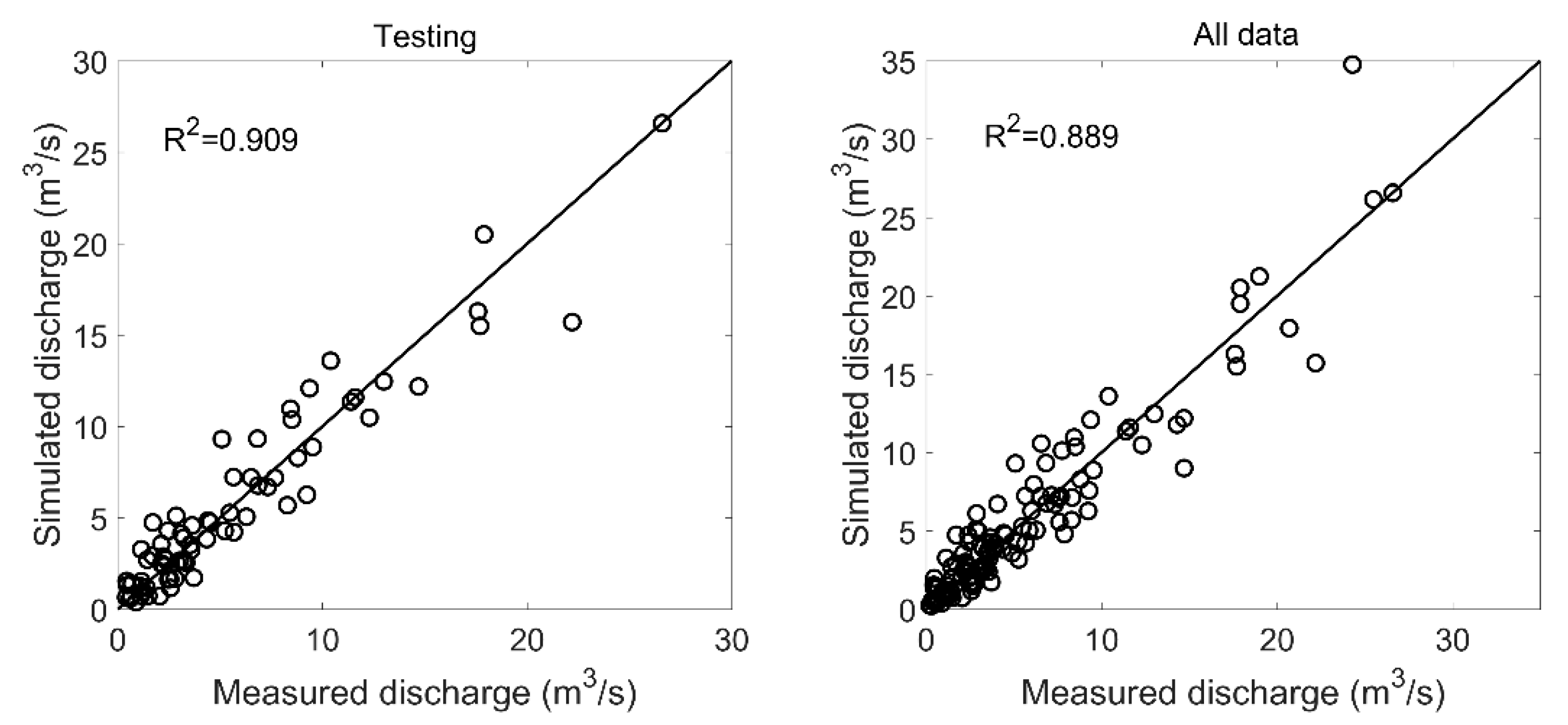
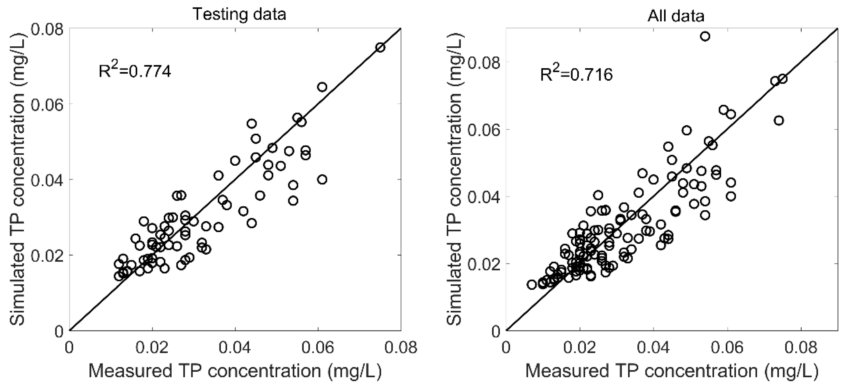
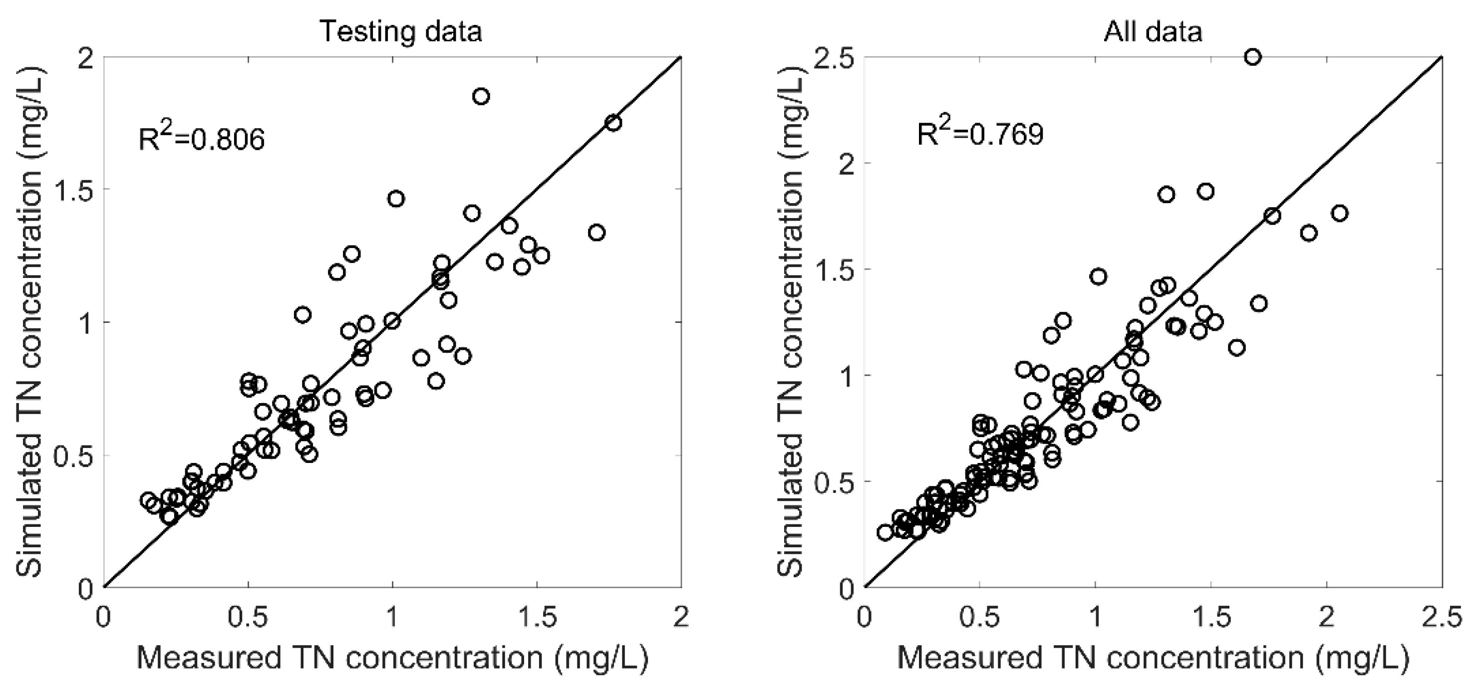
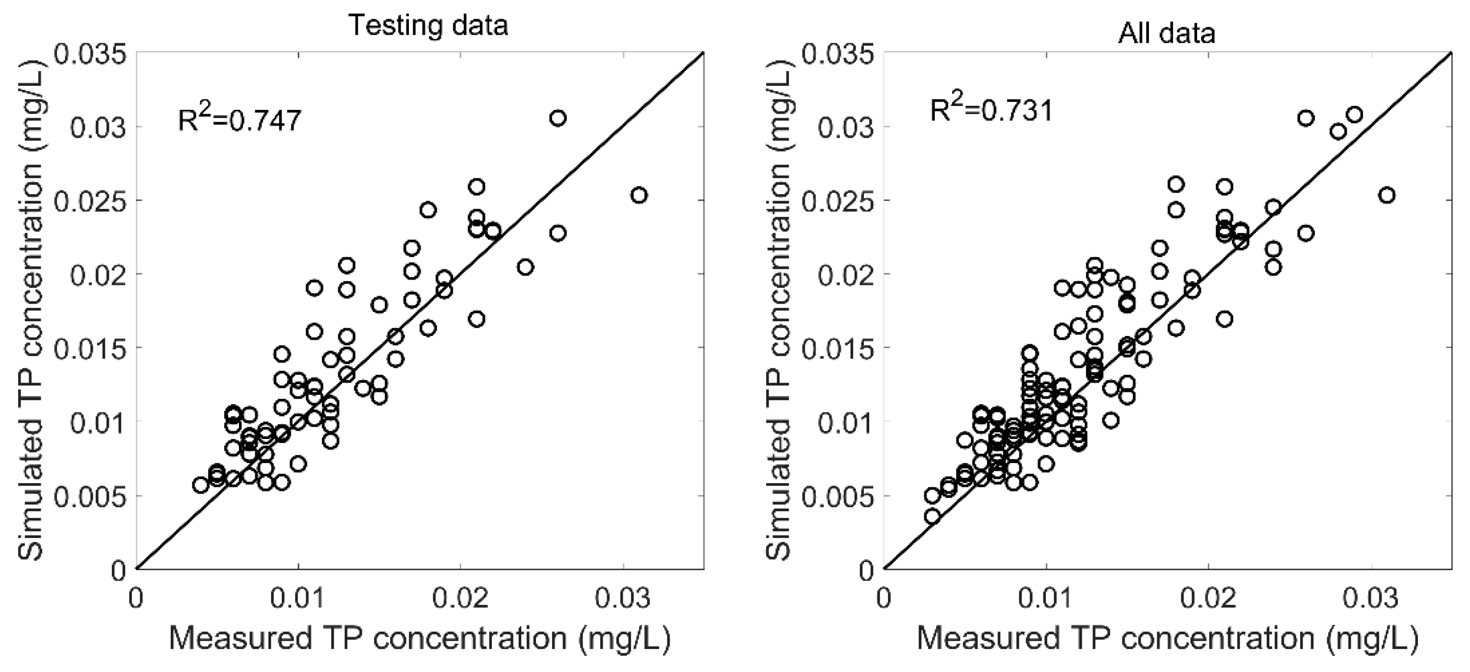
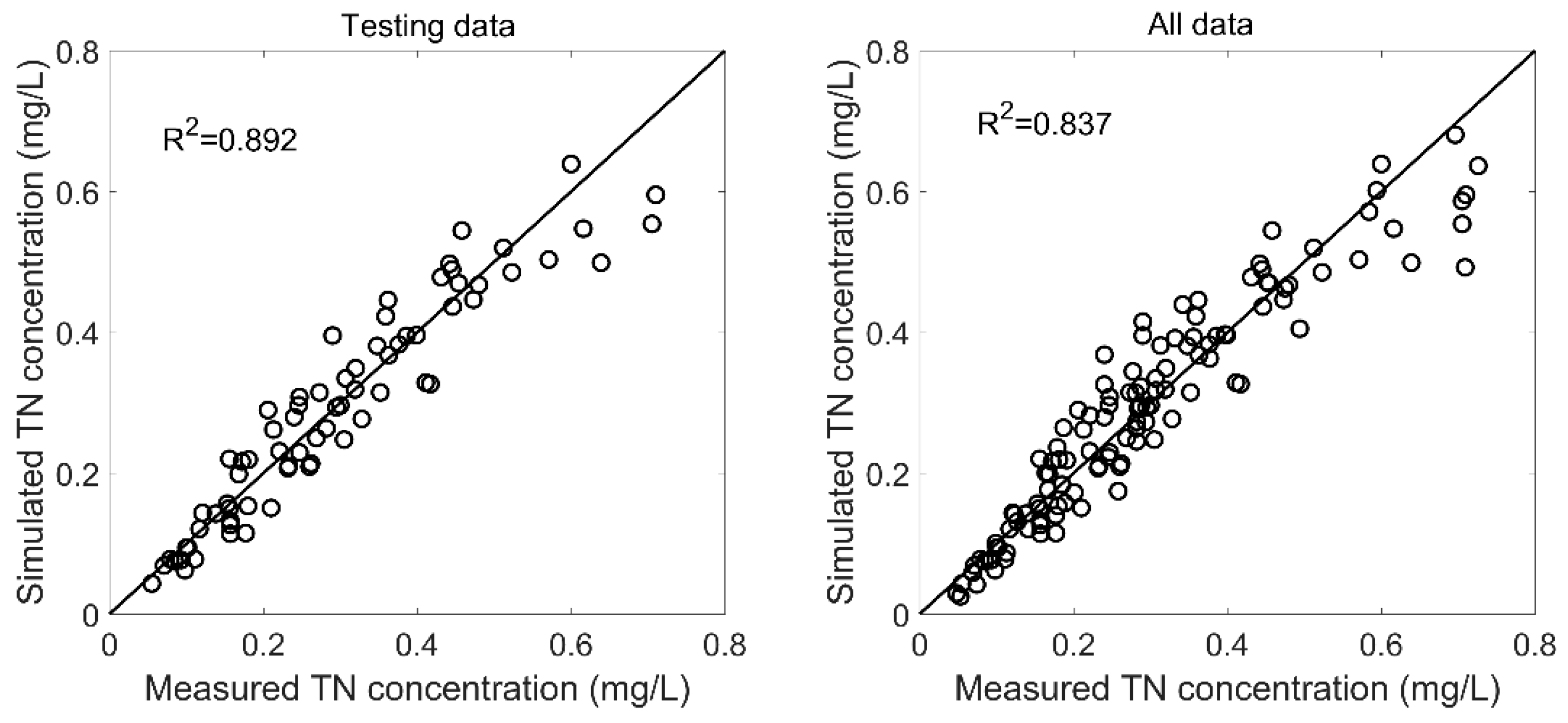
3.2. The Analysis of the Optimal Result

The simulation results of various parameters are shown in

Table 2. The optimal formula of each parameter.

Parameter	Complexity	MAE	Formula
$Q$	9	1.167	$\frac{Q}{Q_{max}}=0.7028\times R/R_{max}+0.604\times R/R_{max}{}^2$
$T{P}_{inlet}$	5	0.0056	$\frac{T{P}_{inlet}}{T{P}_{inletmax}}=0.1707+0.9971\times R/R_{max}$
$T{N}_{inlet}$	9	0.1295	$\frac{T{N}_{inlet}}{T{N}_{inletmax}}=0.1127+1.578\times R/R_{max}+0.533\times \frac{Q}{Q_{max}}$
$T{P}_{outlet}$	9	0.0023	$\frac{T{P}_{outlet}}{T{P}_{outletmax}}=0.2252+1.0355\times \frac{T{P}_{inlet}}{T{P}_{inletmax}}+0.0702\times \frac{Q}{Q_{max}}$
$T{N}_{outlet}$	6	0.03922	$\frac{T{N}_{outlet}}{T{N}_{outletmax}}=\frac{R}{R_{max}}/\left(0.3399+0.726\frac{R}{R_{max}}\right)$

. It can be seen that high simulation accuracy has been achieved when the complexity of the simulation is between 5 and 9. The relationship between attack complexity and accuracy is shown in Figure 7. We choose the time when the complexity increases but the accuracy increases little. The simulation accuracy of each formula testing data and the simulation accuracy of all data are shown in Figure 8, Figure 9, Figure 10, Figure 11 and Figure 12. It can be seen that the simulation effect of each formula is relatively good, and the R² of testing data is 0.909, 0.774, 0.806, 0.747, and 0.892, respectively. The R² of all data is 0.889, 0.716, 0.769, 0.731, and 0.837, respectively.

4. Discussion

By analyzing the relationship between correlations (Table 1), we can see that the relationship between rainfall and runoff is very significant. This is also consistent with previous studies. Runoff is mainly caused by rainfall, which can be used to calculate runoff [36,37,38,39]. Through the correlation analysis, it can be found (Table 1) that the correlation between the nitrogen and phosphorus concentration produced by rainfall and runoff is very high, which can be predicted according to the relevant fitting formula (Table 2). This is also consistent with previous studies, which show that a large amount of sediment and nutrients are usually carried away after runoff caused by rainfall [39,40,41]. These sediment and nutrients are the main reasons for affecting the water quality of the reservoir. However, this paper focuses on the impact of rainfall on nutrient loss. In fact, the influencing factors of nutrient loss may also include rainfall intensity, soil texture, slope, farming conditions, protective measures and other factors [42,43,44,45], but the biggest impact is rainfall, so our fitting formula has high accuracy. However, if we want to continue to improve the accuracy in the future, we can substitute these factors into our model and collect more reservoir data to verify the model.

For large lakes and reservoirs, the internal change in nitrogen and phosphorus concentrations is a complex process, which is related to runoff and nitrogen and phosphorus in the runoff, as well as the temperature, pH, wind speed and other related factors of the lake. The simulation of its change process needs to consider the model of complex conditions [46,47,48]. For the small reservoir studied in this paper, the influence of hydrodynamic changes caused by temperature and wind speed on the change in nitrogen and phosphorus concentration in the reservoir is not great (Table 1). Only analyzing rainfall can better predict the change in nitrogen concentration in the reservoir, and only analyzing runoff and phosphorus concentration in runoff can better predict the change in phosphorus concentration in the reservoir. This probably is due to the small water volume of the small reservoir, frequent water release and storage, and the release of endogenous pollutants in the reservoir being far lower than that of exogenous pollutants. These machine learning models with relatively simple structures are mainly based on weather data (such as rainfall). With the development of weather prediction models [49,50], the accuracy of rainfall prediction is getting higher and higher, so it is feasible to use rainfall to predict future reservoir water quality.

Future climate scenario data can be obtained from GCMs, which are provided by the World Climate Research Program (WCRP) of Coupled Model Inter-comparison Project phase 6 (CMIP6, https://esgf-node.llnl.gov/search/cmip6/ (accessed on 15 January 2021)) [51,52]. At the same time, it is also conducive to the management of the reservoir to deduce the water quality of the reservoir according to meteorological predictions. If the water quality of the reservoir does not meet the irrigation and water supply requirements, it is necessary to allocate water from other reservoirs to ensure the normal production and life of people.

In reservoirs, the current velocities are generally low and the water residence time usually ranges from a few weeks to several months or more than one year. Therefore, reservoirs provide us with a time-integrated response to the external forcing [53,54]. In our research, the residence time is not considered and it should be added to the prediction model in future research. At the same time, the Yangmeiling reservoir is mainly used for urban water supply and agricultural water supply, which have high requirements for water quality. This paper only discusses the laws of TN and TP, and other parameters that need to meet the Environmental Quality Standards for Surface Water (GB 3838-2002) should also be fully discussed in future research.

In the catchment of the Yangmeiling Reservoir, the response of the discharge on rainfall is very fast and also that of TP and TN. It means that there is not much storage capacity in the catchment and erosion is quite relevant to the TP and TN concentrations. In other reservoirs with catchments with large hydrologic storage capacity, e.g., lowland regions having thick aquifers, the result will be different from ours. It would be a further substantial limitation for our results on these reservoirs. Chlorophyll concentration and turbidity are highly related to drinking water production [55]. In future research, we will add chlorophyll measurement to the monitoring plan inside the reservoir to establish its relationship with rainfall, flow and water quality, so as to better help reservoir management.

Our method is mainly based on machine learning, it reflects exactly the conditions of the investigated location during the period of data collection. When there are changes in these conditions, e.g., because of changes in the land use in the catchment area, in the hydrologic conditions due to the establishment of big water abstractions or due to climate change or construction of a reservoir upstream, etc., the identified model no longer applies and it will take several years (>5) to collect enough data to establish a new model that is able to reflect the new conditions. At the same time, to apply our results to other reservoirs, we also need to collect a certain amount of data in that reservoir before establishing the equation. If changes in the conditions in the catchment and reservoir are occurring gradually, adaptive learning of the model based on permanently collected monitoring data may overcome the limitation of the application of the model in case of changes. However, in case of rapid and strong changes in the conditions, the model is losing its predictive power and fully new data collection is needed. Moreover, the very limited transferability of a particular model from one water body to another remains. The model does not intend to provide a model for short-term predictions, since they based their model on monthly data and their problems in handling daily data are one more limitation of their approach.

5. Conclusions

Through ten years of long-term hydrological and water quality observation and analysis, the water quality change law and prediction method of the Inside reservoir is determined. The main results are as follows:

(1)

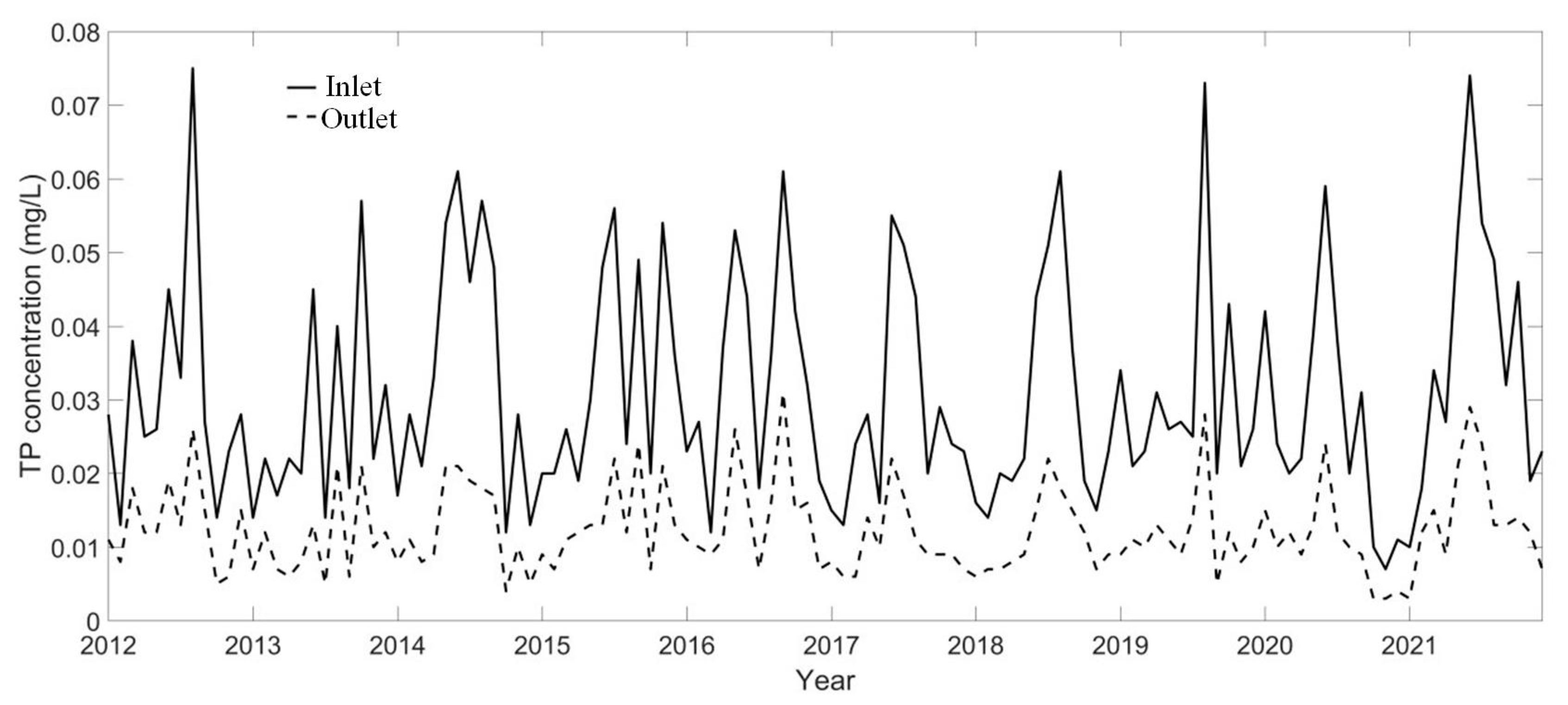
The analysis shows that runoff and the nitrogen and phosphorus content in the runoff have a very significant relationship with rainfall, and the formula related to rainfall can be used to predict runoff and nitrogen and phosphorus concentration.

(2)

It is found that the nitrogen and phosphorus content of the Inside reservoir is less than the nitrogen and phosphorus concentration in the runoff and can also be obtained by using the relevant formula with rainfall, runoff and pollutant concentration content in the runoff. The simple formula is more conducive to the promotion and application of the model and does not provide a theoretical basis for the water quality management of small reservoirs.

References

1. Zhang, S.; Zeng, Y.; Zha, W.; Huo, S.; Niu, L.; Zhang, X. Spatiotemporal variation of phosphorus in the Three Gorges Reservoir: Impact of upstream cascade reservoirs. Environ. Sci. Pollut. Res. 2022, 29, 56739–56749. [Google Scholar] [CrossRef] [PubMed]
2. Winston, B.; Scott, J.T.; Pollock, E. The synergistic effect of elevated CO2 and phosphorus on reservoir eutrophication. Lake Reserv. Manag. 2016, 32, 373–385. [Google Scholar] [CrossRef]
3. Lima, D.J.N.; Menezes, R.F.; Araújo, F.O. Phosphorus fractions and their availability in the sediments of eight tropical semiarid reservoirs. J. Soils Sediments 2022, 22, 982–993. [Google Scholar] [CrossRef]
4. Lu, T.; Chen, N.; Duan, S.; Chen, Z.; Huang, B. Hydrological controls on cascade reservoirs regulating phosphorus retention and downriver fluxes. Environ. Sci. Pollut. Res. 2016, 23, 24166–24177. [Google Scholar] [CrossRef]
5. Khare, Y.; Naja, G.M.; Stainback, G.A.; Martinez, C.J.; Paudel, R.; van Lent, T. A Phased Assessment of Restoration Alternatives to Achieve Phosphorus Water Quality Targets for Lake Okeechobee, Florida, USA. Water 2019, 11, 327. [Google Scholar] [CrossRef] [Green Version]
6. Bai, Y.; Gao, J.; Zhang, Y. Research on wind-induced nutrient release in Yangshapao Reservoir, China. Water Supply 2020, 20, 469–477. [Google Scholar] [CrossRef]
7. Xu, Z.; Yu, C.; Sun, H.; Yang, Z. The response of sediment phosphorus retention and release to reservoir operations: Numerical simulation and surrogate model development. J. Clean. Prod. 2020, 271, 122688. [Google Scholar] [CrossRef]
8. Dang, C.; Lu, M.; Mu, Z.; Li, Y.; Chen, C.; Zhao, F.; Cheng, Y. Phosphorus fractions in the sediments of Yuecheng Reservoir, China. Water 2019, 11, 2646. [Google Scholar] [CrossRef] [Green Version]
9. Huang, L.; Fang, H.; He, G.; Jiang, H.; Wang, C. Effects of internal loading on phosphorus distribution in the Taihu Lake driven by wind waves and lake currents. Environ. Pollut. 2016, 219, 760–773. [Google Scholar] [CrossRef]
10. Shi, W.; Zhu, L.; Van Dam, B.; Smyth, A.R.; Deng, J.; Zhou, J.; Pan, G.; Yi, Q.; Yu, J.; Qin, B. Wind induced algal migration manipulates sediment denitrification N-loss patterns in shallow Taihu Lake, China. Water Res. 2022, 209, 117887. [Google Scholar] [CrossRef]
11. Hu, Y.; Peng, Z.; Zhang, Y.; Liu, G.; Zhang, H.; Hu, W. Air temperature effects on nitrogen and phosphorus concentration in Lake Chaohu and adjacent inflowing rivers. Aquat. Sci. 2022, 84, 33. [Google Scholar] [CrossRef]
12. Gibbons, K.J.; Bridgeman, T.B. Effect of temperature on phosphorus flux from anoxic western Lake Erie sediments. Water Res. 2020, 182, 116022. [Google Scholar] [CrossRef] [PubMed]
13. Bai, Y.; Zeng, Y.; Nie, B.; Jiang, H.; Zhang, X. Hydrodynamic disturbance on phosphorus release across the sediment–water interface in Xuanwu Lake, China. Water Supply 2019, 19, 735–742. [Google Scholar] [CrossRef]
14. Wells, S.A.; Berger, C.J. Modeling the response of dissolved oxygen to phosphorus loading in Lake Spokane. Lake Reserv. Manag. 2016, 32, 270–279. [Google Scholar] [CrossRef]
15. Katsev, S. When large lakes respond fast: A parsimonious model for phosphorus dynamics. J. Great Lakes Res. 2017, 43, 199–204. [Google Scholar] [CrossRef]
16. Yang, X.; Ji, G.; Wang, C.; Zuo, J.; Yang, H.; Xu, J.; Chen, R. Modeling nitrogen and phosphorus export with InVEST model in Bosten Lake basin of Northwest China. PLoS ONE 2019, 14, e0220299. [Google Scholar] [CrossRef] [PubMed]
17. Du, C.; Li, Y.; Lyu, H.; Liu, N.; Zheng, Z.; Li, Y. Remote estimation of total phosphorus concentration in the Taihu Lake using a semi-analytical model. Int. J. Remote Sens. 2020, 41, 7993–8013. [Google Scholar] [CrossRef]
18. Han, H.J.; Los, F.J.; Burger, D.F.; Lu, X.X. A modelling approach to determine systematic nitrogen transformations in a tropical reservoir. Ecol. Eng. 2016, 94, 37–49. [Google Scholar] [CrossRef]
19. Yosri, A.; Siam, A.; El-Dakhakhni, W.; Dickson-Anderson, S. A Genetic Programming–Based Model for Colloid Retention in Fractures. Groundwater 2019, 57, 693–703. [Google Scholar] [CrossRef]
20. Bai, Y.; Yang, J.; Sun, G.; Zhao, Y.; Yu, Y. A genetic programming-based model for predicting phosphorus concentration in shallow lakes. Water Pract. Technol. 2022, 17, 637–644. [Google Scholar] [CrossRef]
21. Sriworamas, K.; Kangrang, A.; Thongwan, T.; Prasanchum, H. Optimal Reservoir of Small Reservoirs by Optimization Techniques on Reservoir Simulation Model. Adv. Civ. Eng. 2021, 2021, 6625743. [Google Scholar] [CrossRef]
22. Chao, J.Y.; Zhang, Y.M.; Kong, M.; Zhuang, W.; Wang, L.; Shao, K.; Gao, G. Long-term moderate wind induced sediment resuspension meeting phosphorus demand of phytoplankton in the large shallow eutrophic Lake Taihu. PLoS ONE 2017, 12, e0173477. [Google Scholar] [CrossRef] [PubMed] [Green Version]
23. Zhu, G.; Qin, B.; Gao, G. Direct evidence of phosphorus outbreak release from sediment to overlying water in a large shallow lake caused by strong wind wave disturbance. Chin. Sci. Bull. 2005, 50, 577–582. [Google Scholar] [CrossRef]
24. Shinohara, R.; Imai, A.; Kohzu, A.; Tomioka, N.; Furusato, E.; Satou, T.; Sano, T.; Komatsu, K.; Miura, S.; Shimotori, K. Dynamics of particulate phosphorus in a shallow eutrophic lake. Sci. Total Environ. 2016, 563, 413–423. [Google Scholar] [CrossRef] [PubMed]
25. Tammeorg, O.; Niemistö, J.; Möls, T.; Laugaste, R.; Panksep, K.; Kangur, K. Wind-induced sediment resuspension as a potential factor sustaining eutrophication in large and shallow Lake Peipsi. Aquat. Sci. 2013, 75, 559–570. [Google Scholar] [CrossRef]
26. Maceina, M.J.; Soballe, D.M. Wind-related limnological variation in Lake Okeechobee, Florida. Lake Reserv. Manag. 1990, 6, 93–100. [Google Scholar] [CrossRef]
27. Kamiya, H.; Ohshiro, H.; Tabayashi, Y.; Kano, Y.; Mishima, K.; Godo, T.; Yamamuro, M.; Mitamura, O.; Ishitobi, Y. Phosphorus release and sedimentation in three contiguous shallow brackish lakes, as estimated from changes in phosphorus stock and loading from catchment. Landsc. Ecol. Eng. 2011, 7, 53–64. [Google Scholar] [CrossRef]
28. Spears, B.M.; Carvalho, L.; Paterson, D.M. Phosphorus partitioning in a shallow lake: Implications for water quality management. Water Environ. J. 2007, 21, 47–53. [Google Scholar] [CrossRef]
29. Søndergaard, M.; Jensen, J.P.; Jeppesen, E. Role of sediment and internal loading of phosphorus in shallow lakes. Hydrobiologia 2003, 506, 135–145. [Google Scholar] [CrossRef]
30. Selig, U.; Hübener, T.; Michalik, M. Dissolved and particulate phosphorus forms in a eutrophic shallow lake. Aquat. Sci. 2002, 64, 97–105. [Google Scholar] [CrossRef]
31. Koza, J.R. Human-competitive results produced by genetic programming. Genet. Program. Evolvable Mach. 2010, 11, 251–284. [Google Scholar] [CrossRef] [Green Version]
32. Schmidt, M.; Lipson, H. Eureqa (Version 0.995 Beta); Nutonian: Somerville, MA, USA, 2003. [Google Scholar]
33. Koza, J.R. Genetic programming as a means for programming computers by natural selection. Stat. Comput. 1994, 4, 87–112. [Google Scholar] [CrossRef]
34. Tinoco, R.O.; Goldstein, E.B.; Coco, G. A data-driven approach to develop physically sound predictors: Application to depth-averaged velocities on flows through submerged arrays of rigid cylinders. Water Resour. Res. 2015, 51, 1247–1263. [Google Scholar] [CrossRef]
35. Liu, M.Y.; Huai, W.X.; Yang, Z.H.; Zeng, Y.H. A genetic programming-based model for drag coefficient of emergent vegetation in open channel flows. Adv. Water Resour. 2020, 140, 103582. [Google Scholar] [CrossRef]
36. Peel, M.C.; McMahon, T.A. Historical development of rainfall-runoff modeling. Wiley Interdiscip. Rev. Water 2020, 7, e1471. [Google Scholar] [CrossRef]
37. Tao, Z.; Li, M.; Si, B.; Pratt, D. Rainfall intensity affects runoff responses in a semi-arid catchment. Hydrol. Process. 2021, 35, e14100. [Google Scholar] [CrossRef]
38. Gao, J.; Bai, Y.; Cui, H.; Zhang, Y. The effect of different crops and slopes on runoff and soil erosion. Water Pract. Technol. 2020, 15, 773–780. [Google Scholar] [CrossRef]
39. Bai, Y.; Cui, H. An improved vegetation cover and management factor for RUSLE model in prediction of soil erosion. Environ. Sci. Pollut. Res. 2021, 28, 21132–21144. [Google Scholar] [CrossRef] [PubMed]
40. Liu, J.; Gao, G.; Wang, S.; Jiao, L.; Wu, X.; Fu, B. The effects of vegetation on runoff and soil loss: Multidimensional structure analysis and scale characteristics. J. Geogr. Sci. 2018, 28, 59–78. [Google Scholar] [CrossRef] [Green Version]
41. López-Vicente, M.; Calvo-Seas, E.; Álvarez, S.; Cerdà, A. Effectiveness of Cover Crops to Reduce Loss of Soil Organic Matter in a Rainfed Vineyard. Land 2020, 9, 230. [Google Scholar] [CrossRef]
42. Barrena-González, J.; Rodrigo-Comino, J.; Gyasi-Agyei, Y.; Pulido, M.; Cerdá, A. Applying the RUSLE and ISUM in the Tierra de Barros Vineyards (Extremadura, Spain) to Estimate Soil Mobilisation Rates. Land 2020, 9, 93. [Google Scholar] [CrossRef] [Green Version]
43. Keesstra, S.D.; Rodrigo-Comino, J.; Novara, A.; Giménez-Morera, A.; Pulido, M.; Di Prima, S.; Cerdà, A. Straw mulch as a sustainable solution to decrease runoff and erosion in glyphosate-treated clementine plantations in Eastern Spain. An assessment using rainfall simulation experiments. Catena 2019, 174, 95–103. [Google Scholar] [CrossRef]
44. Moradi, E.; Rodrigo-Comino, J.; Terol, E.; Mora-Navarro, G.; Marco da Silva, A.; Daliakopoulos, I.N.; Cerdà, A. Quantifying Soil Compaction in Persimmon Orchards Using ISUM (Improved Stock Unearthing Method) and Core Sampling Methods. Agriculture 2020, 10, 266. [Google Scholar] [CrossRef]
45. Jiang, C.; Zhang, H.; Zhang, Z.; Wang, D. Model-based assessment soil loss by wind and water erosion in China’s Loess Plateau: Dynamic change, conservation effectiveness, and strategies for sustainable restoration. Glob. Planet. Change 2019, 172, 396–413. [Google Scholar] [CrossRef]
46. Bhagowati, B.; Ahamad, K.U. A review on lake eutrophication dynamics and recent developments in lake modeling. Ecohydrol. Hydrobiol. 2019, 19, 155–166. [Google Scholar] [CrossRef]
47. Zhang, Q.; Jin, J.; Zhu, L.; Lu, S. Modelling of water surface temperature of three lakes on the Tibetan Plateau using a physically based lake model. Atmos. Ocean 2018, 56, 289–295. [Google Scholar] [CrossRef]
48. Guo, M.; Zhuang, Q.; Yao, H.; Golub, M.; Leung, L.R.; Pierson, D.; Tan, Z. Validation and Sensitivity Analysis of a 1-D Lake Model Across Global Lakes. J. Geophys. Res. Atmos. 2021, 126, e2020JD033417. [Google Scholar] [CrossRef]
49. Hunt, B.G.; Dix, M.R. Stochastic implications for long-range rainfall predictions. Clim. Dyn. 2017, 49, 4189–4200. [Google Scholar] [CrossRef]
50. Jain, S.; Scaife, A.A.; Mitra, A.K. Skill of Indian summer monsoon rainfall prediction in multiple seasonal prediction systems. Clim. Dyn. 2019, 52, 5291–5301. [Google Scholar] [CrossRef]
51. Xiao, D.; Li Liu, D.; Feng, P.; Wang, B.; Waters, C.; Shen, Y.; Tang, J. Future climate change impacts on grain yield and groundwater use under different cropping systems in the North China Plain. Agric. Water Manag. 2021, 246, 106685. [Google Scholar] [CrossRef]
52. O’Neill, B.C.; Tebaldi, C.; van Vuuren, D.P.; Eyring, V.; Friedlingstein, P.; Hurtt, G.; Sanderson, B.M. The scenario model intercomparison project (ScenarioMIP) for CMIP6. Geosci. Model Dev. 2016, 9, 3461–3482. [Google Scholar] [CrossRef] [Green Version]
53. Perga, M.E.; Maberly, S.C.; Jenny, J.P.; Alric, B.; Pignol, C.; Naffrechoux, E. A century of human-driven changes in the carbon dioxide concentration of lakes. Glob. Biogeochem. Cycles 2016, 30, 93–104. [Google Scholar] [CrossRef] [Green Version]
54. Schindler, D.W. Recent advances in the understanding and management of eutrophication. Limnol. Oceanogr. 2006, 51, 356–363. [Google Scholar] [CrossRef] [Green Version]
55. Garrido, M.; Cecchi, P.; Malet, N.; Bec, B.; Torre, F.; Pasqualini, V. Evaluation of FluoroProbe® performance for the phytoplankton-based assessment of the ecological status of Mediterranean coastal lagoons. Environ. Monit. Assess. 2019, 191, 204. [Google Scholar] [CrossRef]
Figure 1. The situation of the study area (1 presents Hongjiata monitoring station at the inlet of reservoir; 2 presents Yangmeiling monitoring station at the inside of reservoir).
Sustainability 14 13755 g001
Figure 2. The monthly average wind speed in the last ten years. The horizontal lines above and below the data points represent error bars.
Sustainability 14 13755 g002
Figure 3. The monthly average air temperature in the last ten years. The horizontal lines above and below the data points represent error bars.
Sustainability 14 13755 g003
Figure 4. The monthly average discharge and monthly sum rainfall of Inlet monitoring station in last ten years.
Sustainability 14 13755 g004
Figure 5. The TP concentration of Inlet and Inside monitoring station in last ten years.
Sustainability 14 13755 g005
Figure 6. The TN concentration of Inlet and Inside monitoring station in last ten years.
Sustainability 14 13755 g006
Figure 7. The relationship between MAE and complexity (a) presents the simulated result of discharge at Inlet monitoring station, (b) presents the simulated result of TP concentration at Inlet monitoring station, (c) presents the simulated result of TN concentration at Inlet monitoring station, (d) presents the simulated result of TP concentration at Inside monitoring station, (e) presents the simulated result of TN concentration at Inside monitoring station.
Sustainability 14 13755 g007
Figure 8. The simulated result of discharge at Inlet monitoring station of testing data and all data.
Sustainability 14 13755 g008
Figure 9. The simulated result of TP concentration at Inlet monitoring station of testing data and all data.
Sustainability 14 13755 g009
Figure 10. The simulated result of TN concentration at Inlet monitoring station of testing data and all data.
Sustainability 14 13755 g010
Figure 11. The simulated result of TP concentration at Inside monitoring station of testing data and all data.
Sustainability 14 13755 g011
Figure 12. The simulated result of TN concentration at Inside monitoring station of testing data and all data.
Sustainability 14 13755 g012