Selected Economic Determinants of Labor Profitability in Family Farms in Poland in Relation to Economic Size

Abstract

Farms in Poland come in a wide variety of sizes, and the effect of farm size on the profitability of labor has not been sufficiently investigated. This paper takes a fresh look at the model for labor profitability determinants of family farms in Poland in relation to their economic size. The purpose of this paper is to analyze the factors that determine the labor profitability index in farms of various economic size classes (classes ES1–ES5). In the analysis of factors shaping the profitability of labor in family farms, a panel analysis was applied. Family farm income expressed per family labor unit was adopted as the dependent variable. The following variables were used as explanatory variables: (1) macroeconomic index of price relations (“price gap”); unemployment; average monthly gross wages and salaries; inflation; (2) technical-agricultural production efficiency index; (3) microeconomic ratio of total assets to agricultural land; technical equipment for work; land-to-labor ratio; debt ratio, subsidy ratio, and investment effort. A diversified influence of selected factors determining the level of profitability of labor in agriculture in particular groups of farms was found. The econometric models developed also indicate different strategies that are adopted by farmers on various farms. There is no single solution here; strategies for improving the profitability of work must take into account the specificity of a given entity. The models estimated indicate the necessity of using other mechanisms and tools of agricultural policy for farms of various economic sizes. It should be expected that, in the future, there will be a dichotomous development of farms. Medium-sized farms will become larger and economically effective, and smaller farms will perform residential functions, with the disappearing function of agricultural production.

1. Introduction

Family farming is widely touted as the most “sustainable” form of agricultural production. Its contribution to social, environmental and economic development is emphasized, ensuring the most efficient food production, positive environmental impacts, and the management of family labor, which contributes to rural economic development [1].

The profitability of labor in agriculture is the result of the value of income generated in agriculture and the level of employment in this sector. The level of labor profitability is particularly important in European agriculture, where family farms play a dominant role. They are relevant to achieving the objectives of the European Union’s common agricultural policy and also to ensuring the existence of a sustainable agricultural sector and rural areas. There are about 10.3 million farms in the European Union (1.41 million in Poland) [2], with an annual working unit (AWU) (Appendix A) of around 9.0 million (1.6 million AWU in Poland), of which about 81% fall under the family farm labor force [3].

A specific feature of EU agriculture is also the predominance of farms with small utilized agricultural areas. The average farm in the EU-28 had 16.6 ha of UAA (utilized agricultural area) in 2016 (in Poland, 10.2 ha). Most farms in the EU-28 are small in physical terms, two-thirds of the EU’s farms were less than 5 ha UAA in size in 2016 and only 7% had more than 50 ha of utilized agricultural areas in 2016 [4]. Comparisons to other nations are as follows: U.S.A.—190 ha; Brazil—46 ha; Chile—52 ha; Canada—281 ha; Argentina—367 ha; Australia—more than 2600 ha per farm [5]. The small scale of production in the majority of farms in the European Union Member States is considered to be one of the main factors that limit the possibilities of improving farming efficiency, including labor profitability [6]. Taking into account the level of family farm income per annual work unit (AWU) compared to wages in the rest of the economy in the EU, it constitutes, on average, only about 45%. Such a large difference between the level of farmers’ income and wages in the rest of the economy, on the one hand, is a social problem related to the poverty of farmers and, on the other hand, limits the development opportunities of farms and may contribute to their bankruptcy, threatening the sustainability of rural areas. The low profitability of labor in agriculture threatens the sustainable development of farms. This is an existential problem for farmers and their families, but it is also a threat to the sustainable development of rural areas and the natural environment.

It is worth noting that the assessment of the importance of the existence of small farms for regions’ social sustainability and biodiversity in many locations of the world is perceived as crucial [7]. There is also some evidence that emissions and resource use efficiency are lower in such farms than they are in middle-sized farms [8,9], especially in low-income countries [10].

The bankruptcy of family farms or the limitation of their development opportunities may cause undesirable effects in rural areas, such as the depopulation of rural areas, the loss of biodiversity, the disappearance of folk culture, the impoverishment of the rural population, etc., but they also pose a threat to food security [11,12,13,14,15,16,17,18,19,20,21,22]. For this reason, the EU’s agricultural policy places great emphasis on ensuring a fair standard of living for the rural population, especially by increasing the individual income of people working in agriculture. The development of the factors determining the level of profitability of labor is important from the point of view of the possibility of shaping appropriate agricultural policy instruments adapted to various types of farms which differ in terms of the scope of production, the direction of production, the degree of connection with the market, etc. The literature regarding the profitability of the farms revolves primarily around the factors that influence the absolute level of agricultural income or its changes over time [23,24,25,26]. According to our knowledge, there is a lack of research regarding the determinants of the profitability of family labor in agriculture, especially taking into account the multi-criteria approach, concerning macroeconomic, microeconomic and technical factors. The degree of agricultural income without reference to the degree of employment of the family workforce is not sufficient to provide a reliable view of the economic situation of the farms. Therefore, despite the high level of agricultural income connected with overly high levels of the use of the family workforce, the costs of the farmer’s own labor and that of their family may not be covered. Such a situation may cause a decline in the standard of living of the farmer’s family and limit the development possibilities of the farm. Hence, from the point of view of the agricultural policy, it is crucial to develop the appropriate instruments to improve the efficiency of using the family workforce in agriculture. The impact of agricultural policy instruments can be twofold. On the one hand, it should aim for the stabilization of the agricultural income, whereas, on the other hand, it should aim for the conditions for the management of surplus labor outside agriculture. The assessment of income support and farm development with subsidies in the EU countries is not clear. It is indicated that the subsidy calculated per output unit is much higher in small farms [27,28]. Moreover, in small farms, subsidies are allocated mainly to financing consumption and not to financing development [29]. Despite that, subsidies supporting the development of small- and medium-sized farms are necessary due to the lack of farmers’ own capital. In some EU countries, insufficient support for farm development leads to the liquidation of a large part of small farms [30].

The literature suggests that the economic size of a farm is of great importance in shaping economic results and management efficiency in agriculture [31,32,33]. Larger entities are able to manage risk and have easier access to credit [34]. As a result, it may lead to a greater stabilization of revenues [35]. The research also points to the fact that the size of farms has a statistically insignificant impact on the variability of income in low-developed countries [36,37,38]. For developed countries, including the countries of the European Union, such as those from the former Soviet bloc, numerous studies show that, with the increase in the size of farms, land and labor productivity and income per working person usually increase [34,39,40,41,42]. Moreover, there is a constant decrease in the number of farms and the concentration of land and labor [22,43]. For this reason, the problem of the influence of the economic size of a farm is included in the scope of the research related to the analysis of the relationship between the farm size and its economic situation and, in the case of this paper, labor profitability.

In the literature on the subject, there is no strict definition of a “small”, “medium” or “large” farm. There are various ways to classify farms [44]. The paper adopts the classification of farms according to the economic size commonly used in the EU (economic size of holding expressed in EUR 1000 of standard output on the basis of the community typology). This measure is widely used for statistical and policy purposes within the EU. This measure determines the size of the farm, its production potential and its production possibilities. This measure has an advantage over the measure of farm size expressed in the area of the agricultural land. In this way, you avoid errors resulting from the incorrect assignment of farms with a small area but which carry out intensive industrial agricultural production (e.g., production in greenhouses, fattening poultry or pigs) to small farms. Therefore, in our research paper, we use economic size.

2. Review of the Literature

2.1. General Aspects of Income and Labor Profitability in Agriculture

There are many trends in the research in the field of income in agriculture. These are review studies [45] and methodological studies [18,46] that take into account the impact of agricultural policy [24], but the main emphasis in the research is on economic factors [25,47]. The analysis of factors determining agricultural income is complicated due to the fact that the set of potential variables is very broad. Therefore, research on the determinants of agricultural income requires a specific research perspective [48]. The research carried out in this paper is part of the analysis of economic factors determining agricultural income, focusing on the profitability of labor.

The profitability of labor is of fundamental importance in assessing the efficiency of managing family farms. It is the level of labor profitability that determines the competitiveness of farms, the level of capital accumulation, their development abilities as well as the level of consumption of farm families [49,50]. In agriculture in developed countries, a change in the implementation of production factor prices is observed. In particular, there is a relative increase in labor costs compared to the other factors: land and, above all, capital [51,52]. This results in the need to improve the use of the labor factor in terms of its productivity and profitability.

The profitability of labor in the family farm should be defined as a relation between the agricultural income generated by the family farm and the resources of the family labor force. Hence, improvements in labor profitability can be obtained by increasing the level of farm income or by reducing the resources of the family labor force. The reduction in the family labor force is mainly related to the possibility of taking up employment outside of agriculture and obtaining income from non-agricultural activity [53], which is especially important for small farms and needier farmers [54,55]. This possibility depends largely on the factors in the surrounding area of the farms. On the other hand, the second way to improve the profitability of labor is related to the increase in agricultural income. It is conditioned by many factors related both to the surroundings of the farm and to the changes taking place in the farm.

The factors shaping the level of labor profitability in family farms are found both in the farm environment (exogenous factors) and inside the farm (endogenous factors). The exogenous factors include macroeconomic, socio-cultural and institutional factors, especially agricultural policy, or factors related to the natural environment and climate [25,56,57,58,59]. In turn, the group of endogenous factors includes the farm size, the resources and relations of production factors, the quality of human capital, managerial abilities, the relation of the farmer’s family to the farm, applied production technologies, etc. [26,60,61,62].

The economic perspective is of particular importance in the research on the determinants of labor profitability in agriculture. From this point of view, three areas can be distinguished [63]: (1) macroeconomic area, (2) technical area, (3) microeconomic area.

2.2. Macroeconomic Determinants of Income in Agriculture

In the macroeconomic area, in economic research, models are constructed in which independent variables are, inter alia, relations between the prices of products sold by farmers to the prices of the means of agricultural production, the costs of factors of production, the exchange rate, interest rates (monetary policy), the GDP level, the economic situation, international trade conditions, the unemployment rate, global financial and economic crises, etc. [25,64,65,66,67,68,69,70]. In the literature on the subject, special attention is paid to macroeconomic factors, as they influence the decisions of agricultural producers and allow one to better understand both the causes and the consequences of changes in farm income. The economic situation of farms will depend on the level of these factors, as well as the strength and direction of their impact [50]. The knowledge of the strength and direction of the impact of these factors is also necessary to shape appropriate agricultural policy instruments correcting their unfavorable impact on agriculture [71]. Moreover, the question arises whether the impact of these factors is the same on the economic situation of various types of farms, especially in countries such as Poland, where small family farms characterized by a weak connection with the market and which produce for their own needs prevail. Therefore, the macroeconomic factors may have a weaker impact on small-scale farms and a greater impact on farms producing on a larger scale, which supply most of their production to the market. Therefore, their responses to changes in macroeconomic parameters may be more sensitive.

2.3. Technical Determinants of Income in Agriculture

Among the factors from the technical area, the relations between the level of agricultural income and the indicators of technical agricultural production efficiency are considered. An improvement in the technical efficiency of farming is a necessary condition to increase economic efficiency. Technological progress has been the most crucial factor in the growth of productivity in agriculture in the new EU member states in recent decades [72]. Moreover, in these countries, an increase in productivity was achieved in a situation of pressure to reduce the consumption of inputs in agriculture [73]. Technological progress and the availability of new agricultural production technologies are the main factors responsible for changes in the technical area of the functioning of farms [74]. However, as a result of the technology treadmill effect occurring in agriculture in the long run, the main beneficiaries of technological progress in agriculture are consumers, not agricultural producers [13,75,76]. Empirical evidence suggests that increases in welfare due to technological advances in agriculture are captured as consumer surplus rather than producer surplus. Ultimately, farmers may find themselves in a worse situation than before the change in production technology. The implementation of technological progress is a necessity, and its effect in the long term is the removal of small farms of poor economic condition from the market. Moreover, technical progress in agriculture has the effect of forcing the labor force out of agriculture, which, in turn, leads to a reduction in the number of people working in agriculture and an improvement in labor profitability [39,77]. However, in order for this effect to be effective, the phenomenon of the labor pull of the agricultural labor force must also occur. The labor pull effect of people working in agriculture largely depends on macroeconomic factors, especially the economic development of the country and the level of unemployment. With a low unemployment rate, the labor pull effect will be strengthened through the labor push effect [38,78,79,80]. Despite the negative consequences of the technology treadmill, farmers are under pressure to implement technological progress. Avoiding new solutions in business practice is impossible. Technical progress allows farmers to reduce unit production costs, increase the scale of production, increase production potential, improve farming efficiency and use environmentally friendly technologies [13]. In this way, it is also possible to limit the unfavorable influence of the price spread between the prices of the final food product and its value as an agricultural raw material on the economic situation of farms [81,82,83,84].

2.4. Microeconomic Determinants of Income in Agriculture

The literature on the subject also highlights the third group of factors that determine the level of agricultural income: endogenous factors, which are mainly microeconomic in nature. It is assumed that, with relatively constant macroeconomic conditions and a constant level of production technologies available, these are the endogenous factors that determine the economic results of farms and the level of efficiency of the resources used. These are factors that largely depend on the farmer [33,85,86]. In the literature of the subject, the following factors are distinguished: the production potential [26,61,87], the value of the farm’s fixed assets [88], the production scale [89], the specialization of farms and the concentration of farm production [36,90,91], the financial situation [17,36,92], the cooperation of farmers [93], the location of farms [92] and human capital [92,94,95]. The set of factors determining farm income and labor profitability is very wide and concerns both quantitative and qualitative aspects. Their significance in shaping the profitability of labor of farms is significant in the short term. In the long term, these are the macroeconomic factors that exert much greater pressure on the financial situation of farms. This pressure forces farmers to change the organizational structure of a farm, the production structure, the relations between production factors and the need to adapt to legal requirements.

In this paper, a multi-criteria approach was applied. In the analysis of the factors determining the profitability of labor in family farms, both macroeconomic as well as technical and microeconomic determinants were taken into account. This approach results from the fact that there are interrelationships between these areas and the feedback pressures between them. The analysis concerns the relationships between macroeconomic, technical and microeconomic factors and the profitability of labor on farms of different economic sizes. This will make it possible to capture the internal differentiation of production structures in agriculture, which determines the need for a different approach to agricultural policy instruments aimed at the development of farms.

3. Materials and Methods

3.1. Objective and Scope of Research

The aim of this paper is to analyze the factors determining the labor profitability index in farms of various economic size classes. The scope of the research included an analysis of the relationship between the labor profitability of a farm and selected macroeconomic, technical and microeconomic indicators.

3.2. Data Source

The analyses were based on the data from two primary sources: (1) mass statistics data and (2) the FADN (Farm Accountancy Data Network) (Appendix A) system for collecting and using farm accountancy data in the EU. Economic and financial data from the FADN system concerned farms operating in the territory of Poland for the period 2004–2020. The time range adopted resulted from the availability of data, and since 2004, farms are based on a standard output according to EU typology. Moreover, since 2004, Poland has been a member of the European Union, and the presented results illustrate the functioning of agriculture in the new economic and political conditions.

3.3. Methods

Panel models are special models built from cross-sectional-temporal data (objects × variables × periods). They describe a fixed group of objects over more than one period. The combination of cross-sectional data and time series contributes primarily to an increase in the number of observations, thus providing more information on the phenomena studied, and this facilitates the establishment of existing relationships between them and their assessment. As a result, it is possible to conduct more in-depth, detailed analyses that cannot be carried out on other types of statistical data. Combining cross-sectional and temporal observations also makes it possible to identify and measure effects that are not observable on typical cross-sectional data or typical time series [96]. The purpose of panel models is to isolate differences between objects that are intrinsically linked to object-specific factors. Therefore, an integral part or even the central issue of the analysis is the heterogeneity of objects [97].

Panel models assume that the formation of the dependent variable is influenced, apart from the explanatory variables, by unmeasured, time-constant and object-specific factors called time effects. Including group and time effects in panel models necessitates specific estimation methods. The extensive use of panel models for econometric analysis is presented by, for example, Baltagi [96], Hsiao [98], Bollen and Brand [99] and Kaddoura and Westerlund [100].

Conducting research using panel analyses also has its limitations. Some difficulties can be encountered at the data collection stage for these analyses, especially if the type of study requires data collection for a balanced panel. A balanced panel is a dataset containing complete data from T periods about each of N units. The longer the analyzed time, the more difficult it is to collect homogeneous data for the same group of objects.

Panel data analysis can be carried out using the ordinary least squares method (OLSM) estimation, the fixed effects model and the random effects model.

Panel models can take the form of models with the decomposition of a constant (FEM—Fixed Effects Model) or models with random component decomposition (REM—Random Effects Model).

In a model estimated using OLSM, the regression occurs on all available observations as if they were cross-sectional data. It is assumed that there are no individual effects (the homogeneity of the community after accounting for differences in the available vector of observable variables X) and no changes in the analyzed phenomenon over time. Under such assumptions, one can treat all observations as if they were from a simple random sample and apply OLSM [101]:

$$y_{it}=X_{it}\beta +v_{it}$$

(1)

where:

• y_it—a dependent variable,
• X_it—an explanatory variable (generally, a vector of explanatory variables),
• β—a vector with the dimension N of structural parameters,
• v_it—total random error, consisting of a purely random part ε_it and an individual effect u_i relating to a specific i-th panel unit (v_it = ε_it + u_i),
• i = 1, 2, …, N—subsequent objects,
• t = 1, 2, …, T—time units.

Fixed Effect Model (FEM). The simplest assumption is that there are constant, unknown (unobservable) but time-constant differences between units:

$$y_{it}=X_{it}\beta +u_i+{\epsilon }_{it}$$

(2)

gdzie:

• u_i—the time-constant individual effect for observations i,
• ε_it—pure random error.

Each individual effect includes all of the time-constant characteristics of an individual that affect the explained variable but are not included explicitly in the vector of explanatory variables due to, for example, the lack of quantifiability or the difficulty of measurement. In a panel model with fixed effects, the determined individual effects are eliminated by averaging the model against time (index t).

Random Effect Model (REM). In a random effects model, each unit is assigned a certain random variable, the realization of which is responsible for the individual effect in a given period. Since individual effects are not the same from period to period, they are not treated as parameters, and their values are not estimated. The total random error, consisting of an individual effect (random effects) and a pure random error v_it = ε_it + u_i, is characterized by a correlation in the same object and a lack of correlation for different objects. It requires the use of a generalized estimator of least squares (GLS) ${\widehat{\beta }}_{RE}$ of structural parameters in the form of [63]:

$${\widehat{\beta }}_{RE}={(X^T{\mathsf{\Omega }}^{-1}X)}^{-1}{X}^T{\mathsf{\Omega }}^{-1}y$$

(3)

where:

• X—a matrix of explanatory variables,
• y—a vector of dependent variables,
• Ω—a reversible matrix of variance and covariance of the total random error.

Specific statistical tests are used to verify panel models:

• The goodness of a model with fixed effects compared to a classic model is verified using the Wald test. The verified null hypothesis assumes that all constants entered into the model are equal, regardless of the object and time. In this case, OLSM should be used.
• The F Test for Individual and/or Time Effects is used to assess the significance of differences between models, assuming the existence or the absence of group effects. The rejection of the null hypothesis assuming the lack of group effects indicates the need to estimate models with fixed effects.
• The Breusch–Pagan test is used to verify the assumption of the constancy of the variance of the random component. The rejection of the null hypothesis indicates the heteroscedasticity of the random component.
• The Hausman test is usually used when choosing between a fixed-effect model and a random-effect model. The null hypothesis is that the individual effects are independent of the explanatory variables, so both estimators are unconstrained. In this case, the estimator for the random effects model is considered more efficient. The opposite situation, on the other hand, means that the estimator for the fixed effects model is unconstrained, while the estimator for the random effects model is constrained. The situation thus indicates that a model with fixed effects is more appropriate.

When choosing between a fixed-effect model and a random-effect model, the nature of the dataset is also important [102]. If the panel contains observations on a fixed and relatively small set of units of interest (e.g., macro-regions in Poland), there is a presumption in favor of fixed effects. In the case of observations on a large number of randomly selected individuals, there is a presumption in favor of random effects. In addition, models with random effects cannot be used if the number of independent variables exceeds the number of units covered by the study.

3.4. Statistical Data

The analysis concerned the impact of selected factors on the level of labor profitability in farms diversified in terms of economic size. The analysis takes into account the farmer’s own labor resources and those of their family and does not include the labor resources employed and paid for by the farmer. The labor profitability index was calculated as a relation of the family farm income to the unpaid labor expressed in FWU (Family Work Unit) (Appendix A). The work profitability analysis concerned farms from six economic size classes (ES1–ES6) (Appendix A) for four macroregions designated for the needs of FADN in Poland. The original intention of the authors was to analyze the profitability of family labor on farms divided into six economic size classes (ES1–ES6). Due to the lack of statistical data on the largest farms (ES6), their analysis was abandoned.

The profitability of labor calculated as the ratio of family farm income (Appendix A) to family work unit [€/FWU] was adopted as the dependent variable— y₁. In the analysis of factors influencing the profitability of labor in family farms, explanatory variables from three areas— macroeconomic, technical and microeconomic—were used. The set of potential explanatory variables belonging to the determinants of labor profitability included:

• Macroeconomic area:

  −

  X₁—the index of price relations (“price gap”) constitutes the ratio of the price index of sold agricultural products to the price index of purchased goods and services. The price indices of sold agricultural products reflect changes in the average weighted procurement prices and the marketplace prices received by farmers. The price indices of purchased goods and services illustrate changes in the retail prices of goods and services purchased for the consumer, current agricultural production or investment purposes. Price indices have been calculated using the structure of the sold agricultural products as well as the structure of purchased goods and services from the year preceding the one under the survey as a weight system. The following weight systems have been applied for goods and services intended for: (1) consumption—the structure of the expenditure (excluding own consumption) of households of farmers resulting from the household budgets survey; (2) current agricultural production—the structure of purchases that were carried out by private farms; (3) investment—the structure of monetary expenditure based on data from national accounts concerning gross capital formation [103]. When this index is greater (less) than 100.0, it indicates that agricultural product (output) prices increase at a faster rate than farm input (commodity) prices, thereby having a positive (negative) effect on farm income. This was estimated for individual regions in Poland and synthetically informs about the economic situation in agriculture.

  −

  X₂—unemployment—registered unemployment rate (for end of year) [%].

  −

  X₃—average monthly gross wages and salaries. This indicator X₂ and X₃ allows for capturing the importance of the process of labor pull from agriculture.

  −

  X₄—price indices of consumer goods and services (inflation).

• Technical area:

  −

  X₅—agricultural production efficiency index, calculated as an output-to-input relation. The costs only represent the total specific costs of agricultural production. The output presents the total output of crops and crop products, livestock and livestock products and other output. The sale and use of (crop and livestock) products and livestock + change in the stock of products + change in the valuation of livestock—purchases of livestock + various non-exceptional products. This index shows the effectiveness of the production technology used and, to a large extent, shows the level of technological advancement of a farm.

• Microeconomic area:

  −

  X₆—ratio of total assets to agricultural land [€/ha]—technical infrastructure of the land,

  −

  X₇—ratio of total assets to the number of people working in the farm [€/AWU] (sum of own and hired labor inputs)—technical equipment for work,

  −

  X₈—land-to-labor [ha/AWU] (AWU—sum of own and hired labor inputs) ratio. These three microeconomic indices (X₆, X₇, X₈) make it possible to take into account the importance of the relationship of production factors in shaping the income situation of a farm. Indirectly, these relations determine the production technique used and reflect the prices of the factors of production.

  −

  X₉—the debt ratio [%] is calculated as the ratio of total liabilities to total assets,

  −

  X₁₀—subsidy ratio [%]—the ratio of the total amount of subsidies to the production value—it depends on the agricultural policy (institutional factor) but also on the farmer’s decision to use specific subsidies (e.g., for public goods provided). The subsidy rate was chosen instead of the simple sum of subsidies because, as indicated by Bojnec and Latruffe [87], it is less correlated with the farm size. In the conditions of the existence of the agricultural support system, it is necessary to take into account the institutional factor, the tangible elements of which are subsidies.

  −

  X₁₁—investment effort calculated as the ratio of gross investment on fixed assets to the sum of depreciation and farm net income. This index informs about the scale of abandoning current consumption in favor of future benefits [104,105].

The above set does not fully exhaust the problem of the determinants of labor profitability, which results from the research approach applied, as well as limitations related to data availability.

4. Results

4.1. Description of Statistical Data

In the macroeconomic area, the four variables presented in Figure 1, Figure 2, Figure 3 and Figure 4 have been highlighted. The price gap (PG) index is used to estimate general price trends and is quite often used by governments to plan, shape and evaluate the effects of agricultural policy. It is also used by farmers to plan the structure and volume of production or to plan investments. It is an index that, to a large extent, can be applied to the analysis of the economic situation in agriculture. Figure 1 presents the value of the price gap in the years 2004–2020. This index was characterized by a relatively high level of changes.

The next two indices adopted as determinants of labor profitability in agriculture in the macroeconomic area are the level of unemployment and the level of remunerations in the national economy (Figure 2 and Figure 3). Both indicators show positive trends in the analyzed period. The unemployment level was characterized by a downward trend, while wages in the national economy were characterized by an increase each year. The increase in wages and salaries in recent years has slowed down, and unemployment was characterized by a low level. This situation should positively affect the level of labor profitability. The decline in unemployment and the growth of remunerations lead to an intensification of the labor pull effect in agriculture, and the impact of this effect may be more significant for smaller farms characterized by under-utilized family labor. Declining unemployment in the national economy pushes the labor force out of the farm. The paper also focused on the level of inflation. This indicator is important because, among other things, it will determine the cost of acquiring capital for the development of farms. Falling inflation has a positive effect on the reduction of the costs of obtaining money from the banking sector and may contribute to stimulating the investment activity of farmers and, consequently, to the development of farms. Inflation data in Poland show a downward trend until 2015. Since 2016, the trend has been reversed (Figure 4).

Table 1. Explained variable and explanatory variables—technical and microeconomic area in 2004–2020.

Variable	ES1	ES2	ES3	ES4	ES5
y1—profitability of labor
$\overline{x}$	1841.32	3786.94	8240.06	14,758.31	32,718.23
Vs (%)	37.84	18.07	18.14	16.30	19.31
As	0.07	0.05	0.18	0.04	0.83
X5—agricultural production efficiency index
$\overline{x}$	3.00	2.70	2.58	2.44	2.16
Vs (%)	12.15	10.35	10.25	8.13	7.12
As	0.20	0.01	0.03	0.01	0.56
X6—technical infrastructure of the land
$\overline{x}$	3312.61	3124.85	3343.23	3589.37	3944.14
Vs (%)	27.83	22.13	24.74	27.79	46.24
As	0.28	−0.14	−0.21	−0.32	0.52
X7—technical equipment for work
$\overline{x}$	21,178.79	27,494.80	43,624.68	63,623.66	78,993.31
Vs (%)	18.63	12.21	9.97	13.69	18.41
As	0.24	0.36	0.02	−0.61	0.19
X8—land-to-labor
$\overline{x}$	6.71	9.22	13.88	19.39	25.59
Vs (%)	21.97	23.72	26.57	34.29	55.36
As	−0.12	0.48	0.77	0.79	0.92
X9—debt ratio
$\overline{x}$	1.63	3.30	6.72	10.99	17.56
Vs (%)	115.80	57.44	48.62	43.04	37.23
As	2.21	0.96	0.82	0.79	0.88
X10—subsidy ratio
$\overline{x}$	36.41	28.28	21.30	16.72	11.13
Vs (%)	38.27	35.84	37.99	40.00	45.75
As	0.53	0.61	0.72	0.65	0.72
X11—investment effort
$\overline{x}$	7.44	23.97	30.29	38.32	41.82
Vs (%)	322.25	129.21	29.35	28.68	43.03
As	3.70	7.56	0.35	0.40	2.81

Source: own elaboration based on the Farm Accountancy Data Network (FADN) (European Commission 2022) [111].

presents selected descriptive statistics of explanatory variables from the microeconomic and technical areas and the dependent variable used for econometric modeling. The variables for all five economic groups under consideration are presented. The profitability of labor clearly increased with the growth of the economic size (Table 1). The largest farms (ES5) were characterized by more than 17 times higher labor profitability than the smallest farms (ES1). These data indicate that small farms are not able to generate a sufficient level of income to cover the costs of their own labor but also to provide prospects for development. In the technical area, the agricultural production efficiency index was taken into account, calculated as the output-to-input ratio (X₅—agricultural production efficiency index) (Table 1). With the increase in the economic size, this index decreased. A similar tendency was found for the capital-to-land ratio (X₆—technical infrastructure of the land). Additionally, farms with a smaller economic size were characterized by a higher level of technical land infrastructure. The situation is different in the case of the technical equipment of work (X₇—technical equipment for work). This index is clearly the lowest in the group of farms by ES1. The changes observed in the relations of production factor prices, consisting in an increase in labor prices in relation to other production factors, result in the need to substitute more expensive labor inputs with relatively cheaper capital [52,107,108]. On the other hand, the ratio of agricultural land per one person employed in a farm (X₈—land-to-labor) was characterized by an increase, along with an increase in the economic size. This situation should be regarded as favorable and conducive to the improvement of management efficiency. The level of farm debt (X₉—debt ratio) clearly increased with the growth in economic size. Small farms use fewer external financing sources. This may limit their exposure to financial risk and reduce the impact of the level of interest rates on their economic situation, but on the other hand, it may contribute to limiting the level of investment and, consequently, the loss of development opportunities. Concerning subsidies (X₁₀—subsidy ratio), we may observe that their proportion of farm revenue is higher among small farms. As the economic size grows, the importance of subsidies declines significantly. This may be caused by the so-called “capping” mechanism, i.e., a limit of the amounts of payment a farm may receive. This index shows that the importance of subsidies and, hence, agricultural policy in shaping the economic situation of small farms is definitely greater than in the case of large farms. The indicator informing about the investment effort of farms (X₁₁—investment effort) is the lowest value, which is significantly different from the remaining groups of farms, in the ES1 group. On average, these farms spent only 7.44% of the sum of depreciation and agricultural income on investments. In the remaining groups of farms, this indicator was definitely higher, and along with the increase in the economic size, this indicator showed an upward trend. It should be assumed that a higher level of this indicator (provided that the level of investment is optimal for a farm) contributes to a higher pace of the development of farms, a faster adaptation to technological changes in agricultural production and an increase in farming efficiency or allows for the release of resources from agricultural to non-agricultural sectors [109,110].

4.2. Results of Econometric Modeling

GRETL and R were used in the econometric modelling of the balanced panel data. Each model was estimated as an ordinary model (OLSM) and a model with fixed effects. The equations were estimated in two analytical forms according to the following equations:

• classic linear panel model:

  $$ESk={\beta }_0+{\beta }_1{X}_1+{\beta }_2{X}_2+{\beta }_3{X}_3+{\beta }_4{X}_4+{\beta }_5{X}_6+{\beta }_7{X}_7+{\beta }_8{X}_8+{\beta }_9{X}_9+{\beta }_{10}{X}_{10}+{\beta }_{11}{X}_{11}+v_i$$

  (4)
• linear fixed effects model:

  $$ESk=u_i+{\beta }_1{X}_1+{\beta }_2{X}_2+{\beta }_3{X}_3+{\beta }_4{X}_4+{\beta }_5{X}_6+{\beta }_7{X}_7+{\beta }_8{X}_8+{\beta }_9{X}_9+{\beta }_{10}{X}_{10}+{\beta }_{11}{X}_{11}+{\epsilon }_i$$

  (5)
• classic exponential panel model:

  $$lnESk={\beta }_0+{\beta }_1{X}_1+{\beta }_2{X}_2+{\beta }_3{X}_3+{\beta }_4{X}_4+{\beta }_5{X}_6+{\beta }_7{X}_7+{\beta }_8{X}_8+{\beta }_9{X}_9+{\beta }_{10}{X}_{10}+{\beta }_{11}{X}_{11}+v_i$$

  (6)
• exponential fixed effects model:

  $$lnESk=u_i+{\beta }_1{X}_1+{\beta }_2{X}_2+{\beta }_3{X}_3+{\beta }_4{X}_4+{\beta }_5{X}_6+{\beta }_7{X}_7+{\beta }_8{X}_8+{\beta }_9{X}_9+{\beta }_{10}{X}_{10}+{\beta }_{11}{X}_{11}+{\epsilon }_i$$

  (7)

For each dependent variable, the four analytical forms listed above were estimated, and the model that better fit the empirical data and the corresponding properties of the random component was selected.

Since the number of independent variables exceeded the number of units covered by the study, models with random effects could not be estimated. The following are the best models of labor profitability in agricultural farms according to their economic size and statistical goodness.

An exponential model with fixed effects was used to build the ES1 (for farm size class ES1) best model (

Table 2. Results of the estimation of the model with fixed effects lnES1.

Variables	Coefficient	Std. Error	t-Ratio	p-Value
const	−6.907680	3.645	−1.895	0.064 *
X1	−0.225046	0.778	−0.289	0.773
X2	−0.011786	0.022	−0.525	0.602
X3	−0.000441	0.000	−2.673	0.010 ***
X4	0.108541	0.030	3.671	0.001 ***
X5	1.001393	0.208	4.820	0.000 ***
X6	0.000188	0.001	0.315	0.754
X7	−0.000021	0.000	−0.236	0.814
X8	0.130750	0.247	0.530	0.598
X9	0.114782	0.053	2.146	0.036 **
X10	0.026099	0.008	3.164	0.003 ***
X11	−0.005063	0.003	−1.818	0.075 *
R2			0.4885	-
F-Statistic			4.6019	0.0001
Wald test (${\chi }^2$)			50.6208	0.0000
F Test for Individual and/or Time Effects			7.9794	0.0002
Breusch−Pagan Test			12.2153	0.3477

* α ≤ 0.1; ** α ≤ 0.05; *** α ≤ 0.01. Source: own elaboration based on the Farm Accountancy Data Network [111].

). This is due to the statistical significance of differences between individual and/or time effects (F Test for Individual and/or Time Effects). In turn, the high value of χ² statistics of Wald’s test confirms the statistical significance of constants. The model describes the variance in the dependent variable at 48.8%, and the value of the F statistic indicates its statistical significance. Five coefficients occurring at variables should be considered statistically significant (α = 0.05): X₃, X₄, X₅, X₉ and X₁₀. An in-depth analysis of the properties of the random component of the model shows that it does not exhibit the property of heteroscedasticity (Breusch–Pagan test).

In the case of the ES2 group of farms, the classic linear panel model, based on the OLS method, was used to describe the profitability of work (

Table 3. Results of the estimation of the classic linear panel model ES2.

Variables	Coefficient	Std. Error	t-Ratio	p-Value
const	−19,467.149	5148.852	−3.781	0.000 ***
X1	3271.970	1416.063	2.311	0.025 **
X2	−43.748	38.163	−1.146	0.257
X3	−0.431	0.265	−1.624	0.110
X4	162.427	43.041	3.774	0.000 ***
X5	759.623	523.467	1.451	0.152
X6	0.166	0.661	0.251	0.803
X7	0.055	0.087	0.630	0.531
X8	215.083	226.599	0.949	0.347
X9	−56.903	96.801	−0.588	0.559
X10	−11.080	17.814	−0.622	0.536
X11	−4.825	2.295	−2.102	0.040 **
R2			0.4801	−
F-Statistic			4.7014	0.0000
Wald test (${\chi }^2$)			51.7154	0.0000
F Test for Individual and/or Time Effects			0.6043	0.6151
Breusch−Pagan Test			20.5465	0.0584

** α ≤ 0.05; *** α ≤ 0.01. Source: own elaboration based on the Farm Accountancy Data Network [111].

). Its correctness of use is indicated by the low value of the F statistic of the test for individual and/or time effects. At the same time, the high value of χ² statistics of Wald’s test indicates the statistical significance of the constant. The discussed model describes the variance in the dependent variable in 48.01%, and the value of the F statistic indicates its statistical significance. Apart from the constant, the three coefficients next to the variables—X₁, X₄, X₁₁—should be considered as statistically significant (α = 0.05). The model does not show heteroscedasticity (Breusch–Pagan test).

In the construction of the ES3 model (

Table 4. Results of the estimation of the model with fixed effects lnES3.

Variables	Coefficient	Std. Error	t-Ratio	p-Value
const	3.375360	1.143	2.952	0.005 ***
X1	0.264986	0.285	0.930	0.357
X2	−0.003672	0.010	−0.371	0.712
X3	−0.000042	0.000	−0.725	0.472
X4	0.034056	0.010	3.471	0.001 ***
X5	0.626949	0.155	4.049	0.000 ***
X6	−0.000172	0.000	−1.339	0.186
X7	0.000045	0.000	3.793	0.000 ***
X8	−0.054220	0.037	−1.455	0.152
X9	−0.001960	0.012	−0.161	0.873
X10	−0.008868	0.006	−1.474	0.146
X11	0.001324	0.002	0.555	0.581
R2			0.7385	-
F-Statistic			13.6087	0.0000
Wald test (${\chi }^2$)			149.6955	0.0000
F Test for Individual and/or Time Effects			7.3285	0.0003
Breusch–Pagan Test			20.0631	0.0545

*** α ≤ 0.01. Source: own elaboration based on the Farm Accountancy Data Network [111].

), an exponential model with fixed effects was used, as indicated by the high value of the F test for individual and/or time effects statistics. The value of the χ² statistics of Wald’s test confirms the statistical significance of constants. The model is fitted to the actual data in 73.58%, and the value of the F statistic indicates its statistical significance. The three coefficients next to the variables—X₃, X₅, X₇—should be considered as statistically significant (α = 0.05). The model does not show heteroscedasticity (Breusch–Pagan test).

The linear model with fixed effects was used to build the ES4 model (

Table 5. Results of the estimation of the model with fixed effects ES4.

Variables	Coefficient	Std. Error	t-Ratio	p-Value
const	−74,505.200	13,556.100	−5.496	0.000 ***
X1	3972.274	3240.871	1.226	0.226
X2	−37.101	103.915	−0.357	0.722
X3	−0.780	0.625	−1.249	0.217
X4	525.521	114.626	4.585	0.000 ***
X5	8516.222	1813.608	4.696	0.000 ***
X6	−0.955	1.093	−0.874	0.386
X7	0.283	0.064	4.432	0.000 ***
X8	129.099	185.932	0.694	0.491
X9	22.305	106.605	0.209	0.835
X10	−189.728	94.864	−2.000	0.051 *
X11	−3.593	22.392	−0.160	0.873
R2			0.7234	-
F-Statistic			12.6030	0.0000
Wald test (${\chi }^2$)			138.6330	0.0000
F Test for Individual and/or Time Effects			6.3502	0.0009
Breusch−Pagan Test			17.5234	0.0933

* α ≤ 0.1; *** α ≤ 0.01. Source: own elaboration based on the Farm Accountancy Data Network [111].

). In this case, high values of the test statistics were recorded for both the Wald test and the F test for individual and/or time effects. The model describes the variance in the dependent variable in 72.34%, and the value of the F statistic indicates its statistical significance. The three coefficients next to the variables—X₄, X₅, and X₇—should be considered as statistically significant (α = 0.05). An in-depth analysis of the properties of the random component of the model shows that it does not exhibit heteroscedastic properties (Breusch–Pagan test).

As in the case of the ES4 model, for the group of the largest farms (ES5), a linear model with fixed effects was used to describe the profitability of work (

Table 6. Results of the estimation of the model with fixed effects ES5.

Variables	Coefficient	Std. Error	t-Ratio	p-Value
const	−115,589.000	40,680.600	−2.841	0.006 ***
X1	14,610.152	9034.753	1.617	0.112
X2	−346.381	288.828	−1.199	0.236
X3	−0.466	2.008	−0.232	0.817
X4	1484.159	355.157	4.179	0.000 ***
X5	6934.137	4669.461	1.485	0.143
X6	0.483	1.257	0.384	0.702
X7	−0.026	0.103	−0.247	0.806
X8	−276.349	314.543	−0.879	0.384
X9	−599.909	234.243	−2.561	0.013 **
X10	−889.734	296.754	−2.998	0.004 ***
X11	16.690	36.076	0.463	0.646
R2			0.4813	-
F-Statistic			4.4716	0.0001
Wald test (${\chi }^2$)			49.1875	0.0000
F Test for Individual and/or Time Effects			5.8291	0.0016
Breusch−Pagan Test			12.8345	0.3043

** α ≤ 0.05; *** α ≤ 0.01. Source: own elaboration based on the Farm Accountancy Data Network [111].

). The necessity of abandoning the use of the classic panel model was indicated by the high values of the test statistics of Wald’s test and the F test for individual and/or time effects. The model describes the variance in the dependent variable at 48.13%, and the value of the F statistic indicates its statistical significance. The three coefficients next to the variables—X₄, X₉ and X₁₀—should be considered as statistically significant (α = 0.05). The test statistics of the Breusch–Pagan test also indicate that the model does not exhibit heteroscedastic properties.

5. Discussion

The analysis of the factors that determine the profitability of work of farms shows the existence of their diversified impact in various groups of farms. Only in the group of the smallest farms (ES1—statistically significant) were dependencies between the labor market and labor profitability recorded (Table 2). A negative impact of the increase in wages in the national economy (average monthly gross wages and salaries) on the labor profitability was found. Rising wages cause the effects of pull labor. This reduces the involvement of the farmer and their family in working on the farm, thus limiting the possibility of increasing agricultural production and income from agricultural activity. The results of this statistical analysis indicate the necessity to use rural development policy instruments that stimulate the creation of jobs outside agriculture. These instruments should be primarily dedicated to the farmers with small farms. The result of such activities should be the improvement of the living conditions of small farmers, as well as the release of land resources that can be used for the development of other farms. The importance of off-farm income is indicated by many authors [112,113,114,115]. Emphasizing the importance of this non-agricultural income in ensuring an adequate standard of living for agricultural families, especially in small farms, attention is drawn to the negative impact on agricultural production and the subsequent positive influence on the purchase of means of production. When analyzing the impact of the labor market on the profitability of work in farms, there is no impact of the unemployment level. Only in the group of the smallest farms did the level of remuneration have a statistically significant impact on the profitability of work. This analysis shows that, in the remaining groups of farms, labor resources can be effectively used on the farm, and it does not necessitate the search for additional sources of income outside the farm. However, it should not be considered that, for other farmers (from farms ES2–ES5), the level of wages outside agriculture does not play an important role (Table 3, Table 4, Table 5 and Table 6). The comparison of agricultural income to wages in the economy is an important aspect that determines the level of job satisfaction on a farm and testifies to the standard of living of farmers. These relationships were not analyzed in the study, which requires further research. Moreover, the lack of a statistically significant impact of the unemployment level, along with the statistically significant influence of the level of wages in the national economy, suggests that farmers take up additional employment if it is possible to obtain satisfactory wages. These data may also indicate the disappearance of the role of small farms in agricultural production in economically developed countries. The decrease in the number of the smallest farms may be beneficial due to the release of resources (especially land) from this type of farms and the taking over of these resources by larger farms. This should stimulate the development of other farms and contribute to the growth of their competitiveness. On the other hand, one should also remember the functions of these farms in rural areas and the public goods they provide [13,116]. This requires further research.

The price indices of consumer goods and services (inflation—X₄) were among the explanatory variables in the macroeconomic area that statistically significantly influenced labor profitability in all analyzed groups of farms. The price indices of consumer goods and services had a positive impact on the level of labor profitability (Table 2, Table 3, Table 4, Table 5 and Table 6). Research by Baek and Koo [117] for farms in the U.S. shows that an increase in the interest rate has a negative impact on the level of agricultural income. 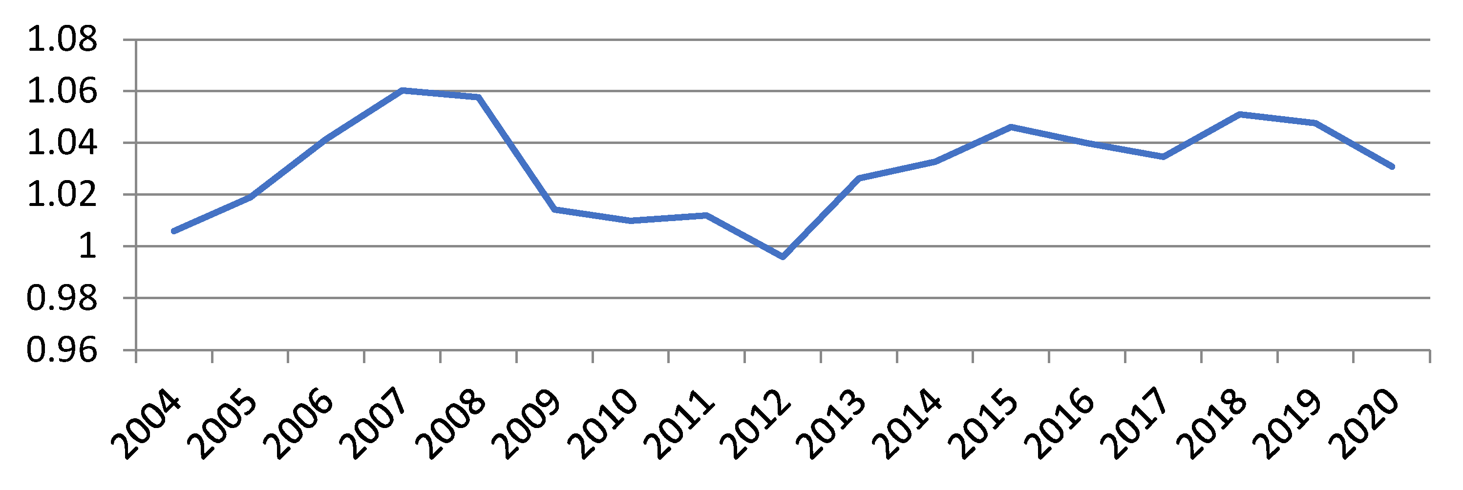Similarly, in the study by Beckman and Schimmelpfennig [25], an increase in the interest rate had a negative impact on the level of agricultural income. The negative relationship between interest rates and agricultural incomes seems obvious, but in our own research, this relationship is reversed. When looking for the reasons for such dependence, attention should be paid to the change in the political situation that Poland experienced after 2004. In 2004, Poland joined the European Union, which had a clear impact on the economic situation in the country. Poland’s accession to the EU improved the situation of farmers in agricultural markets. The downward trends in agricultural commodity prices were reversed, and they stabilized compared to the situation before the accession [84]. Additionally, the prices of food grew at a much faster pace than the prices of non-food products; moreover, in this period, consumer incomes grew much faster than inflation or food prices [118]. These factors contributed to the improvement in the economic situation of farms. Moreover, it should be noted that the level of indebtedness of the analyzed farms was low (Table 1), which did not burden farms with credit costs. Farmers usually reduce the financial risk related to debt, which may inhibit the dynamic development of farms but increase their resistance to financial market disturbances [38,119,120,121].

The macroeconomic variable index of price relations (“price gap”—X₁) had a positive and statistically significant impact on the profitability of labor only in the group of ES2 farms (Table 3). Labor profitability goes up as agricultural commodity prices increase at a faster rate than agricultural input prices. This is confirmed by the results of research by Baek and Koo [117]. Price relations in agriculture are closely related to the profitability of farms. Low and volatile agricultural commodity prices, coupled with ever-increasing agricultural input prices, are the most common economic risks faced by farmers. Similarly, in the studies by Czyżewski et al. [47], attention was drawn to the instability of agricultural product prices, which poses a risk of the destabilization of agricultural income. For this reason, agricultural policy should focus on instruments limiting market risk (ex. revenue and margin insurance) [45,122,123,124,125,126,127,128]. It is also possible to promote collective forms of farmers’ activity or the integration of farmers with agri-food enterprises, which improves the bargaining power of farmers in the market and allows for the possibility of price negotiation.

The agricultural production efficiency index (X₅) was included in the model, explaining the statistically significant work profitability in farms of the size classes ES1, ES3 and ES4. The increase in the value of this index had a positive effect on the profitability of labor. This confirms the dependencies found in many studies by other authors [129,130,131,132,133,134] and points to the need for undertaking actions supporting technological progress in agriculture. In particular, these actions should be focused on smaller farms, as they may have problems with the implementation of new technological solutions due to the limited financial resources. In the group of ES5 farms, no statistically significant relationships were noted, which may indicate a higher level of technological advancement of these farms. These observations are crucial for the policy of supporting investments in farms. Such instruments should be mainly directed toward the medium-sized farms. Larger farms may introduce new technological solutions without financial help from public funds.

Another group of explanatory variables is that of microeconomic indicators that characterize the analyzed farms. Among the micro-economic variables, the technical equipment for work indicator (X₇) had a statistically significant influence on the profitability of labor. At the same time, a statistically significant positive effect of this index was recorded only in the farms of the ES3 and ES4 groups. The importance of modern equipment for the efficient functioning of farms is often emphasized in the literature of the subject [133,135,136]. Moreover, a change in the ratio of prices of production factors (especially dynamically growing labor costs) makes it necessary to replace labor with capital [51,52,107,108]. In the analyzed farms, the process of replacing work with capital had a positive and statistically significant impact on the profitability of work only in farms in the ES3 and ES4 groups (Table 4 and Table 5); in the remaining analyzed groups, no such correlation was noted. This may result from the fact that, in the group of farms ES1 and ES2, the value of technical equipment for work (X₇) was too small (Table 1) to obtain a positive effect of the increase in technical equipment for work. On the other hand, the group of farms ES5 was characterized by the highest level of technical equipment for work, and its further increase did not result in the improvement of management efficiency. These farms (ES5) may have already reached the optimum level of technical equipment for work in relation to their size and production capacity. This is an important observation from the point of view of agricultural policy instruments supporting the investment activity of farmers. This indicates the need to precisely define the support criteria and direct it to a selected group of farms. These results correspond to the above-presented relationships between the profitability of labor and the agricultural production efficiency index (X₅). Further research should also pay attention to the marginal efficiency of capital in various farms. In addition, an important issue is also the quality of machinery and equipment, their degree of modernity, technological advancement and innovation. This requires more detailed research. It is worth noting here that the other two indicators concerning the relationship of production factors (technical infrastructure of the land—X₆ and land-to-labor—X₈) had no statistically significant impact on the profitability of work in the analyzed groups of farms (Table 2, Table 3, Table 4, Table 5 and Table 6).

Among the microeconomic variables, the debt ratio (X₉) was introduced into the model, but only on farms from groups ES1 and ES5. The increase in the debt ratio had a positive impact on labor profitability in ES1 farms, and it had a negative impact in ES5 farms. The financial literature indicates that the growth in debt may have a diversified impact on the financial situation of farms [137,138,139,140,141]. Taking a loan allows for investments and farm development, but too high of a debt level increases the financial risk. In very small farms (ES1), the debt level was low (Table 1), which allowed for the use of the financial leverage effect. In large farms, the level of debt was much higher (Table 1), but it should also be noted that it was not a very high level of debt. Despite this, the increase in indebtedness had a negative impact on the level of work profitability. This may indicate a lower resilience of farms, especially larger ones, to the financial risk related to the growing level of debt. Rising operating costs can burden farms for a long time. Moreover, the specific features of agriculture, resulting from its high dependence on natural, climatic, technological and socio-cultural conditions, affect the specificity of finance in agriculture. In agricultural production, there are usually long production cycles that require pre-financing, leading to a high susceptibility to natural risk. There is a need for specialized machinery and equipment, creating demand for long-term capital and leading to a high volatility of cash flows and economic results. For this reason, it is an important signal for the agricultural policy, indicating the need to mitigate the consequences of credit restrictions in agriculture [142,143,144,145].

In a further analysis, attention was drawn to the relationship between the level of subsidies obtained by farmers as part of state aid and the level of labor profitability. These issues are widely discussed in the literature on the subject, and the conclusions drawn from these studies are not unequivocal. It is indicated that the impact of subsidies on management efficiency, agricultural income and the modernization of agriculture may be positive or negative. It depends on the type of subsidies, the scale of support and the rules for granting subsidies [29,87,146,147,148,149,150,151]. The research also found a diversified influence of operating subsidies on the profitability of work. In the smallest farms (ES1), a statistically significant and positive impact of subsidies on the increase in labor profitability was recorded (Table 2). This is due to the large role of subsidies in shaping the profitability of work (Table 1). In this type of farms, operating subsidies constitute a significant support of agricultural income and may be responsible for the duration of these farms. In the groups of farms ES2 and ES3, operating subsidies did not have a statistically significant impact on the level of work profitability (Table 3 and Table 4). On the other hand, in the largest farms (ES4 and ES5), they had a statistically significant and negative impact on labor profitability (Table 5 and Table 6). This may result from the fact that the decreasing level of subsidies forces farmers to take the trouble of looking for other sources of improving the profitability of work, e.g., in terms of improving the efficiency of farming. Operating subsidies may cause the effect of the “laziness” of farmers, consisting in the lack of motivation to improve the efficiency of the functioning of the farm. It is also emphasized that subsidies are an important decision variable taken into account in the profitability and optimization accounts of farm managers [152], prompting them to behave more riskily. This can also be the cause of negative dependencies between the profitability of work and the level of subsidies. Despite the fact that government support for European agriculture focuses, inter alia, on ensuring an adequate and stable level of income for farming families, the authors’ own research found a diversified impact of agricultural subsidies on labor profitability: positive for very small farms (ES1), negative for large farms (ES5) and no statistically significant correlations in other groups of farms. This indicates a high dependence on the agricultural policy mechanisms of very small farms and a lesser dependence for others. However, this analysis needs to take into account the context of the specificity of Polish agriculture, where very small farms predominate (it is estimated that, out of 1,411,000 farms, only 300–400,000 are potentially developing), which do not produce for the market or occasionally sell their products. For this type of farm, the mechanisms of agricultural policy may be important in shaping agricultural income. In the FADN agricultural accounting system database, commercial farms selling their products on the market are mainly represented. For this reason, the analysis of factors determining the profitability of labor in very small farms of a social nature (production intended for household needs or occasionally sold) requires separate studies that also take into account their role in the social environment related to maintaining the vitality of rural areas and natural environmental benefits (e.g., maintenance of biodiversity). Moreover, the methodology used in the FADN system does not take into account the income obtained by farmers from sources other than agricultural production, which makes the analysis of the income situation difficult [18]. Further research on the impact of subsidies on labor profitability should focus on the structure of obtained subsidies and their role in shaping agricultural income, as well as on their importance in the process of the modernization of farms.

The last microeconomic factor taken into account was the investment effort index (X₁₁). A statistically significant influence of this index on work profitability was found only in the smallest farms (ES1 and ES2). The increase in the investment effort negatively influenced the level of work profitability. This may result from the fact that these farms generate a low level of agricultural income, and the implementation of investments (even small ones) significantly burdens such farms, negatively affecting their financial situation, especially in terms of financial liquidity. Moreover, small farms may implement unprofitable, too small, replacement investments which do not allow for the significant development of the farm, achieving a production scale ensuring a significant increase in agricultural income. This may be related to barriers to the development of such farms, but it requires further research. In the remaining groups of farms, no statistically significant impact of the investment effort index on the level of work profitability was recorded. The investment effort in the farms of the ES3–ES5 groups was much higher than that in the farms of ES1 and ES2. This may result from the fact that these farms implement rational and profitable investments that do not burden the economic result with excessive costs, but due to the presence of a technological treadmill, they cannot have a positive impact on the level of agricultural income [13,75,153].

This article estimates models of labor profitability determinants in farms diversified in terms of economic size. The profitability of labor is one of the basic criteria ensuring the sustainability of a farm and its development possibilities, and it is also a prerequisite to providing a wide range of desired services from agriculture, ranging from the provision of food to environmental goods and services and cultural services [154,155].

A diversified influence of selected factors determining the level of profitability of work in agriculture in particular groups of farms was found. The econometric models developed also indicate different strategies that are adopted by farmers on various farms. There is no single solution here; strategies for improving the profitability of work must take into account the specificity of a given entity.

6. Conclusions

In conclusion, it is worth paying particular attention to the importance of macro-economic factors and agricultural policy. The analysis showed a diversified influence of macroeconomic factors, but in all analyzed groups of farms, a positive influence was found regarding the price indices of consumer goods and services (inflation—X₄). This analysis shows the importance of macroeconomic factors in shaping the work profitability of farms of various economic sizes, both in small and large ones. In the analyzed group of farms, small farms, despite a small scale of production, were present in agricultural markets (they sold their production; they were not farms focused on production for their own needs). Therefore, thanks to contacts with agricultural markets, macroeconomic conditions were transmitted to farms, even the smallest ones. In the context of the impact of macroeconomic factors and the lack of influence of subsidies on labor profitability, it is worth considering the mechanisms of agricultural policy. Admittedly, subsidies increase the level of agricultural income. It cannot be ruled out, however, that, in the conditions of ceasing subsidization, farmers would be forced to improve the efficiency of farming, which would favor an improvement in income. Secondly, in the absence of subsidies, one should expect an increase in the prices of agricultural products and, on the other hand, a decrease in the prices of the means of production. Thus, it can be concluded that part of the payments from the budget of the Common Agricultural Policy of the European Union (CAP) is capitalized not only in land prices but also in price relations (the so-called “price scissors”). It is therefore clear that the potential elimination of the payments would lead to a smaller drop in income than a simple calculation of the subsidy share in income. The European Commission estimates that this decrease would amount to approximately 17% [63]. The research confirmed the influence of the price gap index on the profitability of labor in farms. For this reason, an important tool of agricultural policy should be instruments limiting the market risk related to the volatility of prices in agricultural markets. However, this cannot be achieved by providing guaranteed prices. This direction operated for nearly the first 20 years of CAP, generated high costs and turned out to be ineffective. Currently, attention is drawn to the need to introduce risk management instruments in agriculture, not only in the market but also those related to climate change (e.g., revenue and margin insurance, insufficient area yield and weather index, income insurance).

The obtained results can be the basis for presenting a general conclusion. It seems possible that, in situations of supporting farms with subsidies, the importance of market and economic factors will be minor and will not significantly affect the production and organizational decisions of the farmers running small farms. This is due to the lower income per person in small farms, which results in the need to look for employment outside of agriculture. Moreover, such farms will not be an attractive workplace for farmers’ children, and, due to the lack of successors, they will not develop. There will be a dichotomous development of farms. Medium-sized farms will become larger and economically effective, and smaller farms will perform residential functions, with disappearing agricultural production functions. This is due to the need to incur expenditures on development investments, which might be too heavy of a burden in small farms.

The conducted analysis also indicated the need to pay attention to agricultural policy instruments that promote the implementation of new production technologies and innovative solutions. This leads to an improvement in the profitability of agricultural production, which is positively correlated with the increase in labor profitability. However, such instruments should be mainly directed toward the medium-sized and smaller farms that are potentially developing. Large farms can cope without such support.

The models estimated indicate the necessity of using other mechanisms and tools of agricultural policy for farms of various economic sizes. At the same time, particular attention should be paid to the mechanisms that allow one to limit the exposure to the market risk of farms. The analyses relate to a short period of time; in further studies, it is necessary to pay attention to the influence of the dynamics of changes in macroeconomic, technical and microeconomic factors on the level of profitability of labor in agriculture.

References

1. Fuller, A.M.; Xu, S.; Sutherland, L.-A.; Escher, F. Land to the Tiller: The Sustainability of Family Farms. Sustainability 2021, 13, 11452. [Google Scholar] [CrossRef]
2. Available online: https://ec.europa.eu/eurostat/databrowser/view/ef_m_farmleg/default/table?lang=en (accessed on 6 October 2022).
3. Available online: https://ec.europa.eu/eurostat/databrowser/view/ef_lf_main/default/table?lang=en (accessed on 6 October 2022).
4. Available online: https://ec.europa.eu/eurostat/statistics-explained/index.php?title=Farms_and_farmland_in_the_European_Union_-_statistics#Farms_in_2016 (accessed on 6 October 2022).
5. Available online: https://www.fao.org/faostat/en/#data (accessed on 6 October 2022).
6. Dabkienė, V. The Comparative Analysis of Lithuanian Farms Economic Performance in the Context of Selected EU Countries. Bulg. J. Agric. Sci. 2021, 27, 1074–1083. Available online: https://www.agrojournal.org/27/06-05.pdf (accessed on 11 October 2022).
7. Ricciardi, V.; Mehrabi, Z.; Wittman, H.; James, D.; Ramankutty, N. Higher Yields and More Biodiversity on Smaller Farms. Nat. Sustain. 2021, 4, 651–657. [Google Scholar] [CrossRef]
8. Rada, N.E.; Fuglie, K.O. New Perspectives on Farm Size and Productivity. Food Policy 2019, 84, 147–152. [Google Scholar] [CrossRef]
9. Wicki, L.; Wicka, A. Is the EU Agriculture Becoming Low-Carbon? Trends in the Intensity of GHG Emissions from Agricultural Production. In Proceedings of the 23rd International Scientific Conference Economic Science for Rural Development 2022, Jelgava, Latvia, 11–13 May 2022; Auzina, A., Ed.; Latvia University of Life Sciences and Technologies: Jelgava, Latvia, 2022; Volume 56, pp. 68–78. Available online: https://llufb.llu.lv/conference/economic_science_rural/2022/Latvia_ESRD_56_2022.pdf (accessed on 11 October 2022).
10. Foster, A.D.; Rosenzweig, M.R. Are There Too Many Farms in the World? Labor Market Transaction Costs, Machine Capacities, and Optimal Farm Size. J. Political Econ. 2022, 130, 636–680. [Google Scholar] [CrossRef]
11. Ikerd, J.E. The need for a system approach to sustainable agriculture. Agric. Ecosyst. Environ. 1993, 46, 147–160. [Google Scholar] [CrossRef]
12. Schaller, N. The concept of agricultural sustainability. Agric. Ecosyst. Environ. 1993, 46, 89–97. [Google Scholar] [CrossRef]
13. Kusz, D. Modernization of agriculture vs sustainable agriculture. Sci. Pap. Ser. Manag. Econ. Eng. Agric. Rural Dev. 2014, 14, 171–178. Available online: http://managementjournal.usamv.ro/pdf/vol4_1/Art28.pdf (accessed on 23 August 2022).
14. Sussy, M.; Ola, H.; Maria, F.A.B.; Niklas, B.-O.; Onyango, M.C.; Oluoch-Kosura, W.; Håkan, M.; Djurfeldt, G. Micro-Spatial Analysis of Maize Yield Gap Variability and Production Factors on Smallholder Farms. Agriculture 2019, 9, 219. [Google Scholar] [CrossRef] [Green Version]
15. Poczta-Wajda, A. Economic viability of family farms in Europe—A literature review. Ann. PAAAE 2020, XXII, 161–172. [Google Scholar] [CrossRef]
16. Poczta-Wajda, A.; Sapa, A.; Stępień, S.; Borychowski, M. Food Insecurity among Small-Scale Farmers in Poland. Agriculture 2020, 10, 295. [Google Scholar] [CrossRef]
17. Poczta, W.; Średzińska, J.; Chenczke, M. Economic Situation of Dairy Farms in Identified Clusters of European Union Countries. Agriculture 2020, 10, 92. [Google Scholar] [CrossRef]
18. Runowski, H. Dilemmas of measuring and evaluating income in agriculture in the European Union. Ann. PAAAE 2020, XXII, 289–299. [Google Scholar] [CrossRef]
19. Aydoğdu, M.H.; Cançelik, M.; Sevinç, M.R.; Çullu, M.A.; Yenigün, K.; Küçük, N.; Karlı, B.; Ökten, Ş.; Beyazgül, U.; Doğan, H.P.; et al. Are You Happy to Be a Farmer? Understanding Indicators Related to Agricultural Production and Influencing Factors: GAP-Şanlıurfa, Turkey. Sustainability 2021, 13, 12663. [Google Scholar] [CrossRef]
20. Smędzik-Ambroży, K.; Matuszczak, A.; Kata, R.; Kułyk, P. The Relationship of Agricultural and Non-Agricultural Income and Its Variability in Regard to Farms in the European Union Countries. Agriculture 2021, 11, 196. [Google Scholar] [CrossRef]
21. Suresh, A.; Krishnan, P.; Jha, G.K.; Reddy, A.A. Agricultural Sustainability and Its Trends in India: A Macro-Level Index-Based Empirical Evaluation. Sustainability 2022, 14, 2540. [Google Scholar] [CrossRef]
22. Filipiak, T.; Wicki, L. Is the Structure of Polish Agriculture Changing? A Comparison Based on the Results of Recent General Agricultural Censuses. Ann. PAAAE 2022, XXIV, 37–53. [Google Scholar] [CrossRef]
23. Gardner, B.L. Determinants of farm family income inequality. Am. J. Agric. Econ. 1969, 51, 753–769. [Google Scholar] [CrossRef]
24. Severini, S.; Tantari, A. The impact of agricultural policy on farm income concentration: The case of regional implementation of the CAP direct payments in Italy. Agric. Econ. 2013, 44, 275–286. [Google Scholar] [CrossRef]
25. Beckman, J.; Schimmelpfennig, D. Determinants of farm income. Agric. Financ. Rev. 2015, 75, 385–402. [Google Scholar] [CrossRef]
26. Ryś-Jurek, R. Determinants of family farm income depending on farm size. Ann. PAAAE 2019, XXI, 401–411. [Google Scholar] [CrossRef] [Green Version]
27. Čechura, L.; Žáková Kroupová, Z.; Lekešová, M. Productivity and Efficiency in Czech Agriculture: Does Farm Size Matter? Agric. Econ. (Zemědělská Ekon.) 2022, 68, 1–10. [Google Scholar] [CrossRef]
28. Svobodová, E.; Redlichová, R.; Chmelíková, G.; Blažková, I. Are the Agricultural Subsidies Based on the Farm Size Justified? Empirical Evidence from the Czech Republic. Agriculture 2022, 12, 1574. [Google Scholar] [CrossRef]
29. Bereżnicka, J.; Wicki, L. Do Operating Subsidies Increase Labour Productivity in Polish Farms? Stud. Agric. Econ. 2021, 121, 114–121. [Google Scholar] [CrossRef]
30. Ciutacu, C.; Chivu, L.; Andrei, J.V. Similarities and Dissimilarities between the EU Agricultural and Rural Development Model and Romanian Agriculture. Challenges and Perspectives. Land Use Policy 2015, 44, 169–176. [Google Scholar] [CrossRef] [Green Version]
31. Yan, J.; Chen, C.; Hu, B. Farm size and production efficiency in Chinese agriculture: Output and profit. China Agric. Econ. Rev. 2019, 11, 20–38. [Google Scholar] [CrossRef]
32. Kata, R.; Wosiek, M. Inequality of Income in Agricultural Holdings in Poland in the Context of Sustainable Agricultural Development. Sustainability 2020, 12, 4963. [Google Scholar] [CrossRef]
33. Kryszak, Ł.; Guth, M.; Czyżewski, B. Determinants of farm profitability in the EU regions. Does farm size matter? Agric. Econ.—Czech 2021, 67, 90–100. [Google Scholar] [CrossRef]
34. Ladvenicová, J.; Miklovičová, S. The Relationship between Farm Size and Productivity in Slovakia. Visegr. J. Bioecon. Sustain. Dev. 2015, 4, 46–50. [Google Scholar] [CrossRef] [Green Version]
35. Goddard, E.; Weersink, A.; Chen, K.; Turvey, C.G. Economics of Structural Change in Agriculture. Can. J. Agric. Econ./Rev. Can. D’agroecon. 1993, 41, 475–489. [Google Scholar] [CrossRef]
36. Purdy, B.M.; Langemeier, M.R.; Featherstone, A.M. Financial Performance, Risk, and Specialization. J. Agric. Appl. Econ. 1997, 29, 149–161. [Google Scholar] [CrossRef] [Green Version]
37. Barry, P.J.; Escalante, C.L.; Bard, S.K. Economic risk and the structural characteristics of farm businesses. Agric. Financ. Rev. 2001, 61, 74–86. [Google Scholar] [CrossRef]
38. Foster, A.; Rosenzweig, M.R. Barriers to farm profitability in India: Mechanization, scale and credit markets. In Proceedings of the Conference Agriculture for Development-Revisited, Berkeley, CA, USA, 1–2 October 2010. [Google Scholar]
39. Bojnec, Š.; Fertő, I. Farm Income Sources, Farm Size and Farm Technical Efficiency in Slovenia. Post-Communist Econ. 2013, 25, 343–356. [Google Scholar] [CrossRef]
40. Wicki, L. Size vs Effectiveness of Agricultural Farms. Ann. PAAAE 2019, XXI, 285–296. [Google Scholar] [CrossRef] [Green Version]
41. Sheng, Y.; Chancellor, W. Exploring the Relationship between Farm Size and Productivity: Evidence from the Australian Grains Industry. Food Policy 2019, 84, 196–204. [Google Scholar] [CrossRef]
42. Bojnec, Š.; Fertő, I. The Growth of Farms: A Hungarian-Slovenian Comparison. Post-Communist Econ. 2021, 33, 79–93. [Google Scholar] [CrossRef]
43. Kisielińska, J. Concentration of Production Factors and Support and Their Productivity in EU Farms. Ann. PAAAE 2019, XXI, 204–214. [Google Scholar] [CrossRef] [Green Version]
44. Davidova, S.; Thomson, K. Family Farming in Europe: Challenges and Prospects; European Parliament’s Committee on Agriculture and Rural Development: Brussels, Belgium, 2014; Available online: https://www.europarl.europa.eu/RegData/etudes/note/join/2014/529047/IPOL-AGRI_NT(2014)529047_EN.pdf (accessed on 1 June 2022).
45. Finger, R.; El Benni, N. Farm income in European agriculture: New perspectives on measurement and implications for policy evaluation. Eur. Rev. Agric. Econ. 2021, 48, 253–265. [Google Scholar] [CrossRef]
46. Runowski, H. The problem of assessing the level of agricultural income in European Union. Ann. PAAAE 2017, XIX, 185–190. [Google Scholar] [CrossRef]
47. Czyżewski, A.; Grzelak, A.; Kryszak, Ł. Determinants of income of agricultural holdings in EU countries. In Proceedings of the 2018 VII International Scientific Conference Determinants of Regional Development, Pila, Poland, 12–13 April 2018. [Google Scholar] [CrossRef]
48. Kryszak, Ł.; Staniszewski, J. The fallacy of composition on the example of incomes in European agriculture. In Proceedings of the 2018 VII International Scientific Conference Determinants of Regional Development, Pila, Poland, 12–13 April 2018. [Google Scholar] [CrossRef]
49. Coppola, A.; Scardera, A.; Amato, M.; Verneau, F. Income Levels and Farm Economic Viability in Italian Farms: An Analysis of FADN Data. Sustainability 2020, 12, 4898. [Google Scholar] [CrossRef]
50. Kulawik, J.; Płonka, R.; Wieliczko, B. Changes in the income situation of agricultural holdings in the light of the polish FADN observations from 2004–2018. Probl. Agric. Econ. 2020, 365, 108–134. [Google Scholar] [CrossRef]
51. Hayami, Y.; Ruttan, V.W. Factor prices and technical change in agricultural development: The United States and Japan, 1880–1960. J. Political Econ. 1970, 78, 1115–1141. [Google Scholar] [CrossRef]
52. Runowski, H.; Ziętara, W. Future role of agriculture in multifunctional development of rural areas. Appl. Stud. Agribus. Commer. 2010, 4, 135–143. [Google Scholar] [CrossRef] [PubMed]
53. Haggblade, S.; Hazell, P. Agricultural technology and farm-nonfarm growth linkages. Agric. Econ. 1989, 3, 345–364. [Google Scholar] [CrossRef]
54. Kakungulu, M.; Isabirye, M.; Akoyi, K.T.; Van Hoyweghen, K.; Liesbet Vranken, L.; Maertens, M. Changing income portfolios and household welfare in rural Uganda. Agrekon 2021, 60, 227–242. [Google Scholar] [CrossRef]
55. Lanjouw, J.O.; Lanjouw, P. The rural non-farm sector: Issues and evidence from developing countries. Agric. Econ. 2001, 26, 1–23. [Google Scholar] [CrossRef]
56. Góral, J.; Kambo, K.; Kulawik, J.; Osuch, D.; Płonka, R.; Poczta-Wajda, A.; Soliwoda, M.; Wąs, A. Subsidies versus Economics, Finances and Income of Farms (1); Monographs of Multi-Annual Programme, Institute of Agricultural and Food Economics National Research Institute: Warsaw, Poland, 2015; Available online: https://ssrn.com/abstract=3593217 (accessed on 24 August 2022).
57. Kusz, D.; Gędek, S.; Kata, R. Macroeconomic determinants of the dynamics of investment in agriculture (case of Poland). Sci. Pap. Ser. Manag. Econ. Eng. Agric. Rural Dev. 2015, 15, 171–178. Available online: http://managementjournal.usamv.ro/pdf/vol15_2/Art28.pdf (accessed on 24 August 2022).
58. Czyżewski, A.; Kryszak, Ł. Agricultural income and prices. The interdependence of selected phenomena in Poland compared to EU-15 member states. Manag. Econ. 2017, 18, 47–62. [Google Scholar] [CrossRef] [Green Version]
59. Kryszak, Ł. Agricultural models in EU FADN regions and changes in farm productivity and incomes. J. Agribus. Rural Dev. 2018, 50, 403–413. [Google Scholar] [CrossRef]
60. Kusz, D.; Gędek, S.; Ruda, M.; Zając, S. Endogenous determinants of investments in farms of selected countries of central and Eastern Europe. Sci. Pap. Ser. Manag. Econ. Eng. Agric. Rural Dev. 2014, 14, 107–116. Available online: http://managementjournal.usamv.ro/pdf/vol_14/art16.pdf (accessed on 24 August 2022).
61. Strzelecka, A.; Zawadzka, D.; Kurdyś-Kujawska, A. Production Potential and Income of Agricultural Holdings in Poland. Barom. Reg. 2018, 16, 137–144. Available online: http://br.wszia.edu.pl/zeszyty/pdfs/br53_15strzelecka.pdf (accessed on 24 August 2022). [CrossRef]
62. Grzelak, A.; Staniszewski, J.; Borychowski, M. Income or Assets—What Determines the Approach to the Environment among Farmers in a Region in Poland? Sustainability 2020, 12, 4917. [Google Scholar] [CrossRef]
63. Kryszak, Ł.; Czyżewski, B. Determinanty Dochodów Rolniczych w Regionach Unii Europejskiej (Determinants of Agricultural Income in the Regions of the European Union); CeDeWu: Warsaw, Poland, 2020. [Google Scholar]
64. Schuh, G.E. The exchange rate and US agriculture. Am. J. Agric. Econ. 1974, 56, 1–13. [Google Scholar] [CrossRef]
65. Chambers, R.G. Agricultural and financial market interdependence in the short run. Am. J. Agric. Econ. 1984, 66, 12–24. [Google Scholar] [CrossRef]
66. Orden, D. Exchange rate effects on agricultural trade. J. Agric. Appl. Econ. 2002, 34, 303–312. [Google Scholar] [CrossRef] [Green Version]
67. Baek, J.; Koo, W.W. On the dynamic relationship between US farm income and macroeconomic variables. J. Agric. Appl. Econ. 2009, 41, 521–528. [Google Scholar] [CrossRef] [Green Version]
68. Baek, J.; Koo, W.W. The US agricultural sector and the macroeconomy. J. Agric. Appl. Econ. 2010, 42, 457–465. [Google Scholar] [CrossRef] [Green Version]
69. Rabiei, H.; Salarpour, M.; Sabouhi Saboni, M. Effect of macroeconomic variables on the Iran agricultural sector income. Agric. Econ. Res. 2012, 4, 65–85. [Google Scholar]
70. Martinho, V.J.P.D. Testing for Structural Changes in the European Union’s Agricultural Sector. Agriculture 2019, 9, 92. [Google Scholar] [CrossRef] [Green Version]
71. Martinho, V.J.P.D.; Mourao, P.R.; Georgantzis, N. Efficiency of the European Union farm types: Scenarios with and without the 2013 CAP measures. Open Agric. 2022, 7, 93–111. [Google Scholar] [CrossRef]
72. Wicki, L. The Role of Productivity Growth in Agricultural Production Development in the Central and Eastern Europe Countries after 1991. In Proceedings of the 19th International Scientific Conference Economic Science for Rural Development, Jelgava, Latvia, 9–11 May 2018; Auzina, A., Ed.; Latvia University of Life Sciences and Technologies: Jelgava, Latvia, 2018; Volume 47, pp. 514–523. [Google Scholar] [CrossRef]
73. Wicki, L. The Role of Technological Progress in Agricultural Output Growth in the NMS Upon European Union Accession. Ann. PAAAE 2021, XXIII, 85–99. [Google Scholar] [CrossRef]
74. Barnes, A.P.; Soto, I.; Eory, V.; Beck, B.; Balafoutis, A.; Sánchez, B.; Vangeyte, J.; Fountas, S.; van der Wal, T.; Gómez-Barbero, M. Exploring the Adoption of Precision Agricultural Technologies: A Cross Regional Study of EU Farmers. Land Use Policy 2019, 80, 163–174. [Google Scholar] [CrossRef]
75. Cochrane, W.W. Farm Prices: Myth and Reality; University of Minnesota Press: Minneapolis, MN, USA, 1958. [Google Scholar]
76. Czyżewski, B.; Poczta-Wajda, A. Effects of policy and market on relative income deprivation of agricultural labor. Wieś Rol. 2017, 3, 53–70. [Google Scholar] [CrossRef]
77. Tudor, V.C.; Dinu, T.A.; Vladu, M.; Smedescu, D.; Vlad, I.M.; Dumitru, E.A.; Sterie, C.M.; Costuleanu, C.L. Labour Implications on Agricultural Production in Romania. Sustainability 2022, 14, 8549. [Google Scholar] [CrossRef]
78. Jorgenson, D.W. The Development of a Dual Economy. Econ. J. 1961, 71, 309–334. [Google Scholar] [CrossRef]
79. Kelley, A.C.; Williamson, J.G.; Cheetham, R.J. Dualistic Economics Development: Theory and History; University of Chicago Press: Chicago, IL, USA, 1972. [Google Scholar]
80. Alvarez-Cuadrado, F.; Poschke, M. Structural change out of agriculture: Labor push versus labor pull. Am. Econ. J. Macroecon. 2011, 3, 127–158. [Google Scholar] [CrossRef] [Green Version]
81. Gardner, B.L. The Farm-Retail Price Spread in a Competitive Food Industry. Am. J. Agric. Econ. 1975, 57, 399–409. [Google Scholar] [CrossRef]
82. Riston, C. Agricultural Economics Principles and Policy; Westview: Denver, CO, USA, 1982. [Google Scholar]
83. Chavas, J.-P.; Pan, F. The Dynamics and Volatility of Prices in a Vertical Sector. Am. J. Agric. Econ. 2020, 102, 353–369. [Google Scholar] [CrossRef]
84. Kusz, D.; Kusz, B.; Hydzik, P. Changes in the Price of Food and Agricultural Raw Materials in Poland in the Context of the European Union Accession. Sustainability 2022, 14, 4582. [Google Scholar] [CrossRef]
85. Naschold, F. Microeconomic determinants of income inequality in rural Pakistan. J. Dev. Stud. 2009, 45, 746–768. [Google Scholar] [CrossRef]
86. Rembisz, W.; Bezat-Jarzębowska, A. Microeconomics of Agricultural Producers’ Income; LAP Lambert Academic Publishing: Chisinau, Republic of Moldova, 2013. [Google Scholar]
87. Bojnec, Š.; Latruffe, L. Farm size, agricultural subsidies and farm performance in Slovenia. Land Use Policy 2013, 32, 207–217. [Google Scholar] [CrossRef]
88. Średzińska, J. Determinants of the Income of Farms in EU Countries. Stud. Oecon. Posnaniensia 2018, 6, 54–65. [Google Scholar] [CrossRef]
89. Duffy, M. Economies of Size in Production Agriculture. J. Hunger Environ. Nutr. 2009, 4, 375–392. [Google Scholar] [CrossRef]
90. Albrecht, D.E. The Correlates of Farm Concentration in American Agriculture. Rural Sociol. 1992, 57, 512–520. [Google Scholar] [CrossRef]
91. Mugera, A.; Langemeier, M. Does Farm Size and Specialization Matter for Productive Efficiency? Results from Kansas. J. Agric. Appl. Econ. 2011, 43, 515–528. [Google Scholar] [CrossRef] [Green Version]
92. Schurle, B.; Tholstrup, M. Farm Characteristics and Business Risk in Production Agriculture. Appl. Econ. Perspect. Policy 1989, 11, 183–188. [Google Scholar] [CrossRef]
93. Golovina, S.; Hess, S.; Nilsson, J.; Wolz, A. Networking among Russian farmers and their prospects for success. Post-Communist Econ. 2019, 31, 484–499. [Google Scholar] [CrossRef] [Green Version]
94. Butko, G.P.; Saparova, O.N. Features of using human capital in agrarian sector of economy. Agrar. Bull. Ural. 2021, 212, 73–79. [Google Scholar] [CrossRef]
95. Bratianu, C.; Stanescu, D.F.; Mocanu, R.; Bejinaru, R. Serial Multiple Mediation of the Impact of Customer Knowledge Management on Sustainable Product Innovation by Innovative Work Behavior. Sustainability 2021, 13, 12927. [Google Scholar] [CrossRef]
96. Baltagi, B.H. Econometric Analysis of Panel Data; John Wiley & Sons, Ltd.: Chichester, UK, 2005. [Google Scholar]
97. Greene, W.H. Econometric Analysis; Prentice-Hall, Inc.: Hoboken, NJ, USA, 2003. [Google Scholar]
98. Hsiao, C. Panel data analysis—Advantages and challenges. TEST 2007, 16, 1–22. [Google Scholar] [CrossRef] [Green Version]
99. Bollen, K.A.; Brand, J.E. A General Panel Model with Random and Fixed Effects: A Structural Equations Approach. Soc. Forces 2010, 89, 1–34. [Google Scholar] [CrossRef] [PubMed] [Green Version]
100. Kaddoura, Y.; Westerlund, J. Estimation of Panel Data Models with Random Interactive Effects and Multiple Structural Breaks when T is Fixed. J. Bus. Econ. Stat. 2022, 1–13. [Google Scholar] [CrossRef]
101. Kufel, T. Ekonometria. Rozwiązywanie Problemów z Wykorzystaniem Programu GRETL; Wydawnictwo Naukowe PWN: Warsaw, Poland, 2013. [Google Scholar]
102. Cottrell, A.; Lucchetti, R.J. Gretl User’s Guide. Gnu Regression, Econometrics and Time-Series Library. 2022. Available online: http://gretl.sourceforge.net/gretl-help/gretl-guide.pdf (accessed on 1 July 2022).
103. Statistics Poland. Statistical Yearbook of the Republic of Poland; Statistics: Warsaw, Poland, 2021. Available online: https://stat.gov.pl/obszary-tematyczne/roczniki-statystyczne/roczniki-statystyczne/rocznik-statystyczny-rzeczypospolitej-polskiej-2021,2,21.html (accessed on 3 June 2022).
104. Szymańska, E.J.; Dziwulski, M.; Kruszyński, M. Determinants of Fixed Asset Investment in the Polish Farms. Sustainability 2021, 13, 13741. [Google Scholar] [CrossRef]
105. Kusz, D.; Zając, S.; Dziekan, R. Regional Diversification of Investment Outlays and Labour Profitability in Agriculture in Poland. Ann. PAAAE 2020, XXII, 116–126. [Google Scholar] [CrossRef]
106. Available online: https://stat.gov.pl/obszary-tematyczne/ceny-handel/wskazniki-cen/wskazniki-cen-towarow-i-uslug-konsumpcyjnych-pot-inflacja-/roczne-wskazniki-cen-towarow-i-uslug-konsumpcyjnych (accessed on 4 June 2022).
107. Kislev, Y.; Peterson, W. Prices, Technology, and Farm Size. J. Political Econ. 1982, 90, 578–595. Available online: http://www.jstor.org/stable/1831371 (accessed on 22 August 2022). [CrossRef]
108. Kusz, D. Changes in the Relations of Production Factors in Agriculture (the Case of Poland). Sci. Pap. Ser. Manag. Econ. Eng. Agric. Rural Dev. 2015, 15, 179–188. Available online: http://managementjournal.usamv.ro/pdf/vol15_2/Art29.pdf (accessed on 11 July 2022).
109. Cicea, C.; Subić, J.; Turlea, C. Specific Economic Efficiency Indicators of Investments in Agriculture. J. Cent. Eur. Agric. 2010, 11, 255–263. Available online: https://hrcak.srce.hr/63011 (accessed on 13 July 2022).
110. Donckt, M.V.; Chan, P.; Silvestrini, A. A new global database on agriculture investment and capital stock. Food Policy 2021, 100, 101961. [Google Scholar] [CrossRef]
111. Farm Accountancy Data Network (FADN) European Commission. 2022. Available online: https://agridata.ec.europa.eu/extensions/FADNPublicDatabase/FADNPublicDatabase.html (accessed on 4 June 2022).
112. Mishra, A.K.; Goodwin, B.K. Farm Income Variability and the Supply of Off-Farm Labor. Am. J. Agric. Econ. 1997, 79, 880–887. [Google Scholar] [CrossRef]
113. Alwang, J.; Siegel, P.G. Labor shortages on small landholdings in Malawi: Implications for policy reforms. World Dev. 1999, 27, 1461–1475. [Google Scholar] [CrossRef]
114. Barrett, C.B.; Bezuneh, M.; Aboud, A. Income diversification, poverty traps and policy shocks in Côte d’Ivoire and Kenya. Food Policy 2001, 26, 367–384. [Google Scholar] [CrossRef]
115. Pfeiffer, L.; López-Feldman, A.; Taylor, J.E. Is off-farm income reforming the farm? Evidence from Mexico. Agric. Econ. 2009, 40, 125–138. [Google Scholar] [CrossRef]
116. Bisht, I.S.; Rana, J.C.; Pal Ahlawat, S. The Future of Smallholder Farming in India: Some Sustainability Considerations. Sustainability 2020, 12, 3751. [Google Scholar] [CrossRef]
117. Baek, J.; Koo, W.W. Dynamic Interrelationships between the U.S. Agricultural Trade Balance and the Macroeconomy. J. Agric. Appl. Econ. 2007, 3, 457–470. [Google Scholar] [CrossRef]
118. Seremak-Bulge, J. Zmiany cen i marż cenowych na podstawowych rynkach żywnościowych. Zesz. Nauk. SGGW Ekon. Organ. Gospod. Żywn. 2012, 100, 5–23. Available online: https://sj.wne.sggw.pl/pdf/EIOGZ_2012_n100_s5.pdf (accessed on 5 September 2022).
119. Hubbard, R.G.; Kashyap, A.K. Internal Net Worth and the Investment Process: An Application to U.S. Agriculture. J. Political Econ. 1992, 100, 506–534. Available online: http://www.jstor.org/stable/2138729 (accessed on 26 August 2022). [CrossRef] [Green Version]
120. Barry, P.J.; Bierlen, R.W.; Sotomayor, N.L. Financial Structure of Farm Businesses under Imperfect Capital Markets. Am. J. Agric. Econ. 2000, 82, 920–933. Available online: http://www.jstor.org/stable/1244530 (accessed on 26 August 2022). [CrossRef]
121. Petrick, M. Credit Rationing of Polish Farm Households. A Theoretical and Empirical Analysis; Studies on the Agricultural and Food Sector in Central and Eastern Europe; Institute of Agricultural Development in Central and Eastern Europe IAMO: Halle, Germany, 2004; Volume 26, Available online: https://ageconsearch.umn.edu/record/93022 (accessed on 5 September 2022).
122. Chavas, J.-P. Agricultural policy in an uncertain world. Eur. Rev. Agric. Econ. 2011, 38, 383–407. [Google Scholar] [CrossRef]
123. Bowman, M.S.; Zilberman, D. Economic Factors Affecting Diversified Farming Systems. Ecol. Soc. 2013, 18, 33. Available online: http://www.jstor.org/stable/26269286 (accessed on 26 August 2022). [CrossRef]
124. Glauber, J.W. The growth of the federal crop insurance program, 1990–2011. Am. J. Agric. Econ. 2013, 95, 482–488. [Google Scholar] [CrossRef] [Green Version]
125. Meuwissen, M.P.M.; de Mey, Y.; van Asseldonk, M. Prospects for agricultural insurance in Europe. Agric. Financ. Rev. 2018, 78, 174–182. [Google Scholar] [CrossRef]
126. Meraner, M.; Finger, R. Risk perceptions, preferences and management strategies: Evidence from a case study using German livestock farmers. J. Risk Res. 2019, 22, 110–135. [Google Scholar] [CrossRef]
127. Hazell, P.; Varangis, P. Best practices for subsidizing agricultural insurance. Glob. Food Secur. 2020, 25, 100326. [Google Scholar] [CrossRef]
128. Boháčiková, A.; Bencová, T.; Rábek, T. Comparison of Public Risk Management Tools in Slovak Agriculture. In SHS Web of Conferences; EDP Sciences: Les Ulis, France, 2021; Volume 92. [Google Scholar] [CrossRef]
129. Mishra, A.K.; El-Osta, H.S.; Steele, C.J. Factors Affecting the Profitability of Limited Resource and Other Small Farms. Agric. Financ. Rev. 1999, 59, 77–99. Available online: https://pubag.nal.usda.gov/download/39009/pdf (accessed on 5 September 2022).
130. Rahman, S. Profit efficiency among Bangladeshi rice farmers. Food Policy 2003, 28, 487–503. [Google Scholar] [CrossRef]
131. Pudaka, D.L.; Rusdarti, R.; Prasetyo, P.E. Efficency analysis of rice production and farmers’ income in Sengah Temila District Landak Regency. J. Econ. Educ. 2018, 7, 31–38. Available online: https://journal.unnes.ac.id/sju/index.php/jeec/article/view/22799 (accessed on 27 August 2022).
132. Skarżyńska, A.; Grochowska, R. Determinants of Farm Income Diversification Among the European Union Countries. Zagadnienia Ekon. Rolnej/Probl. Agric. Econ. 2021, 2, 119–134. Available online: https://ssrn.com/abstract=4048007 (accessed on 28 August 2022). [CrossRef]
133. Balafoutis, A.; Beck, B.; Fountas, S.; Vangeyte, J.; Wal, T.V.d.; Soto, I.; Gómez-Barbero, M.; Barnes, A.; Eory, V. Precision Agriculture Technologies Positively Contributing to GHG Emissions Mitigation, Farm Productivity and Economics. Sustainability 2017, 9, 1339. [Google Scholar] [CrossRef] [Green Version]
134. Van Evert, F.K.; Gaitán-Cremaschi, D.; Fountas, S.; Kempenaar, C. Can Precision Agriculture Increase the Profitability and Sustainability of the Production of Potatoes and Olives? Sustainability 2017, 9, 1863. [Google Scholar] [CrossRef] [Green Version]
135. Střeleček, F.; Lososová, J. An evaluation of the types of technical development in agriculture in the years 1995–2000. Agric. Econ.—Czech 2003, 49, 151–165. [Google Scholar] [CrossRef] [Green Version]
136. Balafoutis, A.T.; Evert, F.K.V.; Fountas, S. Smart Farming Technology Trends: Economic and Environmental Effects, Labor Impact, and Adoption Readiness. Agronomy 2020, 10, 743. [Google Scholar] [CrossRef]
137. Greig, B.; Nuthall, P.; Old, K. Resilience and finances on Aotearoa New Zealand farms: Evidence from a random survey on the sources and uses of debt. N. Z. Geogr. 2019, 75, 21–33. [Google Scholar] [CrossRef] [Green Version]
138. Schorr, A.; Lips, M. The optimal capital structure of Swiss dairy farms. Agric. Financ. Rev. 2019, 79, 323–337. [Google Scholar] [CrossRef]
139. Gadanakis, Y.; Stefani, G.; Lombardi, G.V.; Tiberti, M. The impact of financial leverage on farm technical efficiency during periods of price instability. Agric. Financ. Rev. 2020, 80, 1–21. [Google Scholar] [CrossRef]
140. Grashuis, J. Returns to debt and equity in farm producer organizations. Ann. Public Coop. Econ. 2020, 91, 55–69. [Google Scholar] [CrossRef]
141. Ma, W.; Renwick, A.; Zhou, X. The relationship between farm debt and dairy productivity and profitability in New Zealand. J. Dairy Sci. 2020, 103, 8251–8256. [Google Scholar] [CrossRef]
142. Petrick, M. A microeconometric analysis of credit rationing in the Polish farm sector. Eur. Rev. Agric. Econ. 2004, 31, 77–101. [Google Scholar] [CrossRef]
143. Briggeman, B.C.; Towe, C.A.; Morehart, M.J. Credit Constraints: Their Existence, Determinants, and Implications for U.S. Farm and Nonfarm Sole Proprietorships. Am. J. Agric. Econ. 2009, 91, 275–289. [Google Scholar] [CrossRef]
144. Kata, R.; Walenia, A. Financial exclusion of farmers and rural entrepreneurs. J. Agribus. Rural Dev. 2015, 2, 225–235. [Google Scholar] [CrossRef]
145. Kata, R.; Filip, P. European Union subsidies and bank credits as external sources of financing for small and medium enterprises in Poland. Management 2016, 20, 457–472. [Google Scholar] [CrossRef] [Green Version]
146. Poon, K.; Weersink, A. Factors affecting variability in farm and off-farm income. Agric. Financ. Rev. 2011, 71, 379–397. [Google Scholar] [CrossRef] [Green Version]
147. Góral, J. Subsidies and Technical Efficiency of Large-Scale Farms in Poland. Agrarian Perspectives XXIV. Global Agribusiness and the Rural Economy. In Proceedings of the 24th International Scientific Conference, Prague, Czech Republic, 16–18 September 2015; pp. 135–144. Available online: https://spu.fem.uniag.sk/Marian.Toth/publikacie/2015.pdf (accessed on 6 September 2022).
148. Soliwoda, M. The impact of the support instruments of the Common Agricultural Policy on economic and financial stability of farms in EU countries. Acta Univ. Lodz. Folia Oecon. 2016, 2, 99–116. [Google Scholar] [CrossRef]
149. Severini, S.; Tantari, A.; Di Tommaso, G. Do CAP direct payments stabilise farm income? Empirical evidences from a constant sample of Italian farms. Agric. Food Econ. 2016, 4, 6. [Google Scholar] [CrossRef] [Green Version]
150. Bojnec, Š.; Fertő, I. Do CAP subsidies stabilise farm income in Hungary and Slovenia? Agric. Econ. 2019, 65, 103–111. [Google Scholar] [CrossRef] [Green Version]
151. Bereżnicka, J.; Wicki, L. Do Farm Subsidies Improve Labour Efficiency in Farms in EU Countries? Eur. Res. Stud. 2021, XXIV, 925–937. [Google Scholar] [CrossRef]
152. Turvey, C.G. Whole Farm Income Insurance. J. Risk Insur. 2012, 79, 515–540. [Google Scholar] [CrossRef]
153. Czyżewski, B.; Czyżewski, A.; Kryszak, Ł. The Market Treadmill against Sustainable Income of European Farmers: How the CAP Has Struggled with Cochrane’s Curse. Sustainability 2019, 11, 791. [Google Scholar] [CrossRef] [Green Version]
154. Swinton, S.M.; Lupi, F.; Robertson, G.P.; Hamilton, S.K. Ecosystem services and agriculture: Cultivating agricultural ecosystems for diverse benefits. Ecol. Econ. 2007, 64, 245–252. [Google Scholar] [CrossRef]
155. Siebrecht, N. Sustainable Agriculture and Its Implementation Gap—Overcoming Obstacles to Implementation. Sustainability 2020, 12, 3853. [Google Scholar] [CrossRef]
Figure 1. Macroeconomic area—X1—index of price relations (“price gap”), previous year = 100. Sources: [103].
Sustainability 14 13819 g001
Figure 2. Macroeconomic area—X2—unemployment [%]. Sources: [103].
Sustainability 14 13819 g002
Figure 3. Macroeconomic area—X3—the changes in average monthly gross wages and salaries, previous year = 1, fixed prices from 2020. Sources: own calculation based on [103].
Sustainability 14 13819 g003
Figure 4. Macroeconomic area—X4—price indices of consumer goods and services (inflation), previous year = 100. Sources: [106].
Sustainability 14 13819 g004