A Dynamic Dispatching Method for Large-Scale Interbay Material Handling Systems of Semiconductor FAB

Abstract

Interbay Automated Material Handling Systems (AMHS) are widely adopted especially in Semiconductor Wafer Fabrication Systems (SWFS). The dispatching method plays a major role in the control of AMHS. This paper proposes an efficient multi-objective dynamic dispatching method which will dynamically adjust vehicle-load assignments according to the real-time situation of the system. A multi-objective cost function with variable weights is established, taking into account various performance indices (i.e., transport time, throughput, cycle time, vehicle utilization, movement, and waiting time), and the corresponding mathematical model is formulated. Then, in order to obtain the suitable weights according to the real-time condition, an advanced method is developed based on fuzzy theory. After that, a Hungarian algorithm is adopted to solve the model. Finally, simulations are conducted to validate the proposed method. The results demonstrate that it has better comprehensive performance compared to the previous dispatching methods.

1. Introduction

Semiconductor wafer fabrication systems are different from traditional Flow-shop and Job-shop manufacturing systems by many features, such as re-entrant flows, sophisticated processing, mass and mixed work-in-process (WIP), long production cycle times, and high capital investment [1]. Since the wafer size grows from 200 mm to 300 mm, the AMHS has been used in semiconductor manufacturing fabs worldwide [2]. The interbay AMHS is a large-scale, stochastic, dynamic, multi-objective, and re-entrant system, and these features substantially increase the scheduling complexity.

1.1. Scheduling Optimization Problem

Research has been focusing on a scheduling optimization problem. Wong et at. combined the method of given product mix, expected product mix and characteristics of AMHS to generate transportation scheduling patterns [3]. Montoya conducted a survey of wafer fabrication facilities design and automated material handling systems operation and established the optimization objectives such as minimizing the flow time, maximizing the carrier utilization, etc. [4]. In order to improve the overall efficiency of semiconductor manufacturing facilities, Yoon and Chae proposed several effective scheduling strategies for the dispatching of the electrical die sorting (EDS) test facility in the manufacturing process of semiconductor products [5].

Wang proposed a heuristic OHT dispatching rule, which expedited the movement of lots, reduced the waiting time, and minimized the transportation delay in handling [6]. Le-Anh and Koster introduced some single-attribute and multi-attribute dispatching rules [7]. The dispatching rule’s performance was evaluated by using the real-world case study, and the experiment results showed composite rules from multi-attribute dispatching and vehicle reassignment yielded the best performance. An evaluation system based on the mathematical meaning of each index was proposed to study and analyze the performance index of semiconductor system and then obtained the linear relationship between the index [8].

1.2. Real-Time Production Scheduling Problem

These methods mostly used fixed weights and static dispatching rules, which were difficult to meet the demand of multi-objective optimal scheduling of the interbay system. Aiming at the real-time production scheduling problem in the semiconductor manufacturing industry, a self-organizing dynamic scheduling rule is proposed to improve the scheduling efficiency, and the optimal scheduling scheme is automatically generated through interactive methods [9]. Based on system status, a neural network was used to adjust attribute weights. Compared to the same dispatching rule with fixed attribute weights or single attribute rules, their method reached a balance point among different performance measures such as unload cycle time, blocking time, and WIP. With the increase of the demand for embedded flash memory devices, Huh et al. proposed a scheduling device based on artificial neural networks, which effectively reduces the low resource utilization rate, frequent re-entered lots, and long flow time, etc. when producing high-capacity and multi-chip products (MCPS) during the semiconductor wafer manufacturing process [10]. Pan et al. designed a real-time OHT dispatching mechanism, since there were multiple solutions of the scheduling problem with the Hungarian algorithm, and the Hungarian algorithm was improved to distinguish different solutions [11]. The simulation results showed that the real-time OHT dispatching mechanism reduced the average waiting time and average leading time. Li and Min proposed an efficient adaptive dispatching method (ADM), which could adjust parameter weights dynamically according to the real-time state information in fabs [12]. The simulation results showed that compared to the traditional rules, ADM had better performance in adapting to changing environments. Zhang et al. proposed a modified Markov chain model (MMCM) to analyze the performance of a closed-loop automated material handling system with shortcuts and blockings [13]. Zhou and Zhou proposed an impending deadlock detection model and used a graphic formulation with critical chains and shared nodes to effectively avoid impending deadlocks [14]. Their method could be used for high-level deadlocks in AMHSs. Huang et al. proposed a conceptual framework to handle the vehicle allocation problem [15]. Gupta et al. reduced the flow of vehicles, avoided congestion, and reduced cycle time by studying the algorithm of vehicle scheduling in AMHS [16]. Therefore, an effective OHT dispatching rule and differentiated preemptive dispatching (DPD) policy were developed to reduce the impact of OHTs blockages and delivery time, which also minimized the impact of transporting normal lots during the hot lots transportation in a 300 mm OHT system. Wang designed big data analytics (BDA) to predict wafer lots’ cycle time [17]. In addition, a data pre-processing technique was designed to extract, transform, and load data from wafer lot transactions dataset, and a conditional mutual information-based feature selection process was proposed to select key feature subset to reduce the dimension of dataset through analyzing data without pre-knowledge. The results showed that the BDA has higher accuracy than linear regression and back-propagation network in CT forecasting. Lin et al. developed a Markov decision model for vehicle allocation control in AMHS to minimize the sum of the expected waiting time for long-run average transport jobs [18]. Their method reduced the waiting cost for AMHS vehicle transportation significantly. Wang and Chen considered frequent traffic jams when OHT vehicles load and unload in wafer diffusion factories and developed a dispatching rule named heuristic preemptive dispatching rule [19]. Zhang et al. implemented a fuzzy neural network based on a rescheduling decision model in semiconductor manufacturing systems [20]. Their method could quickly choose an optimized rescheduling strategy for semiconductor fabrication lines according to current system disturbances. Li et al. presented an adaptive dispatching rule whose parameters were determined dynamically by the real-time information [21]. In their paper, a backward propagation neural network (BPNN) and a particle swarm optimization (PSO) algorithm were used to identify the relations between parameter weights and real-time information and adapt to these parameters when there was a change. Tyan et al. considered multiple performance measures in a fully automated fab environment and presented an integrated tool and a vehicle dispatching strategy based on these measures [22]. Compared to a static dispatching rule, their rule achieved better performance in measures such as on-time delivery and cycle time. Li et al. considered the effect of OHTs blockages and proposed an OHT reassignment approach based on a Hungarian algorithm [23]. Qin et al. presented a dynamic dispatching method based on a fuzzy logic control to dynamically adjust the weights of the system parameter [24]. This method improved the system efficiency and achieved better overall performance. However, the membership function and fuzzy rules of fuzzy logic were based on expert experience, which has strong subjectivity. Rong and Wang presented an algorithm to extract fuzzy rules directly from the sample data [25]. In order to make up for the lack of expert experience, an advanced method is developed based on fuzzy theory, which can dynamically adjust the parameter weights of the wafer lot’s transportation cost model. The membership functions and rules are obtained from the example data.

1.3. Structure

In this paper, a modified multiple-objective dynamic dispatching method (MMDD) is proposed, which can quickly generate an optimal reassignment policy and adapt to the fast-changing environment. The rule of the dynamic weights adjustment method is not based on prior knowledge but extracted from the sample data. The outline of this paper is organized as follows. The model formulations and the main contents of MMDD are introduced in Section 2 and Section 3, respectively. Section 4 represents the results of simulation. Finally, the conclusions are presented in Section 5.

2. Model Formulations

For 300 mm fabs, a spine AMHS layout is envisioned by the International 300 mm Initiative (I300I). A typical spine-configuration wafer fab layout is illustrated in Figure 1. In this layout, machines are installed in several bays that are connected with a central aisle. Stockers are located at the junctions of the main aisle and each bay [1]. An interbay material handling system includes stockers, loops, and Overhead Shuttle (OHS). Similarly, the intrabay material handling system includes loops, stockers, tools, and Overhead Hoist Transporter (OHT) [26]. Both loops are located overhead to attain zero footprints in transport and minimize the fab footprint. The system transfers the lot from the equipment loading port to the OHT, the OHT transports the lot to the stocker where each bay is located. When the lot needs to be processed, the s1wdv tocker robot transfers the lot to the interbay, and the lot is loaded in the OHS, then the OHS moves the lot to the stocker closest to the next process. OHTs of the intrabay automatically retrieve the lot to the stocker, move it onto the device, and place it on the device’s loading port.

A multi-objective-based mathematical model for scheduling is formulated in this section. The below notations are used in our model.

$dis\left(i,j\right)$	$\mathrm{distance}\mathrm{from}\mathrm{OHS}\mathrm{vehicle}j$$\mathrm{to}\mathrm{the}\mathrm{starting}\mathrm{position}\mathrm{of}\mathrm{lot}i$.
$DU{E}_i$	$\mathrm{due}\mathrm{time}\mathrm{of}\mathrm{wafer}\mathrm{lot}i$.
$AP{T}_i$	$\mathrm{sum}\mathrm{of}\mathrm{processing}\mathrm{time}\mathrm{of}\mathrm{all}\mathrm{operations}\mathrm{for}\mathrm{wafer}\mathrm{lot}i$.
$N_I$	$\mathrm{input}\mathrm{buffer}\mathrm{capacity}\mathrm{of}\mathrm{stocker}k$.
$N_O$	$\mathrm{output}\mathrm{buffer}\mathrm{capacity}\mathrm{of}\mathrm{stocker}k$.
$N$	number of stockers in the interbay system.
$VN$	$\mathrm{number}\mathrm{of}\mathrm{vehicles}\mathrm{in}\mathrm{the}\mathrm{interbay}\mathrm{system}.$
$R{T}_i$	$\mathrm{remaining}\mathrm{time}\mathrm{to}DU{E}_i$.
$P{T}_i$	$\mathrm{sum}\mathrm{of}\mathrm{processing}\mathrm{time}\mathrm{of}\mathrm{all}\mathrm{the}\mathrm{finished}\mathrm{operations}\mathrm{of}\mathrm{wafer}\mathrm{lot}i$.
$w{t}_i$	$\mathrm{time}\mathrm{between}\mathrm{decision}\mathrm{of}\mathrm{wafer}\mathrm{lot}i$ and the arrival of OHS vehicle.
$ni{q}_i$	$\mathrm{input}\mathrm{buffer}\mathrm{queue}\mathrm{length}\mathrm{of}\mathrm{wafer}\mathrm{lot}i$$’s\mathrm{destination}\mathrm{stocker}k$.
$no{q}_i$	$\mathrm{output}\mathrm{buffer}\mathrm{queue}\mathrm{length}\mathrm{of}\mathrm{wafer}\mathrm{lot}i$$’s\mathrm{destination}\mathrm{stocker}k$.
$W{N}_S$	$\mathrm{number}\mathrm{of}\mathrm{waiting}\mathrm{wafer}\mathrm{lots}\mathrm{in}\mathrm{stocker}S$.
$m$	number of waiting wafer lots in the interbay system.
$R{P}_i$	$\mathrm{sum}\mathrm{of}\mathrm{processing}\mathrm{time}\mathrm{for}\mathrm{remaining}\mathrm{operations}\mathrm{of}\mathrm{wafer}\mathrm{lot}i$.
$p$	number of wafer lots that complete all the processing.
$C{T}_i$	$\mathrm{cycle}\mathrm{time}\mathrm{of}\mathrm{wafer}\mathrm{lot}i$.
$c{w}_i$	$\mathrm{average}\mathrm{waiting}\mathrm{time}\mathrm{of}\mathrm{wafer}\mathrm{lot}i$.
$AW$	expected average waiting time.
$\mathrm{Nwt}$	$\mathrm{number}\mathrm{of}\mathrm{wafer}\mathrm{lots}\mathrm{with}\mathrm{waiting}\mathrm{time}\mathrm{greater}\mathrm{than}\mathrm{the}\mathrm{expected}\mathrm{average}\mathrm{waiting}\mathrm{time}\mathrm{AW}$.
$B{S}_{In}$	$\mathrm{input}\mathrm{buffer}\mathrm{level}\mathrm{of}\mathrm{stocker}S$.
$B{S}_{Out}$	$\mathrm{output}\mathrm{buffer}\mathrm{level}\mathrm{of}\mathrm{stocker}S$.
$X_{ij}$	$\mathrm{the}\mathrm{matching}\mathrm{coefficient}\mathrm{matrix},\mathrm{namely}{X}_{ij}$$=\mathrm{binary}\mathrm{for}\mathrm{all}i$$\mathrm{and}j$$.\mathrm{If}\mathrm{lot}i$$\mathrm{is}\mathrm{assigned}\mathrm{to}\mathrm{OHS}j$$\mathrm{then}{X}_{ij}$$=1\mathrm{otherwise}{X}_{ij}$ = 0.
$c_{ij}$	$\cos t\mathrm{value}\mathrm{when}\mathrm{wafer}i$$\mathrm{is}\mathrm{assigned}\mathrm{and}\mathrm{loaded}\mathrm{to}\mathrm{OHS}\mathrm{vehicle}j$.
$C$	cost matrix.

The purpose of the real-time optimization assignment is to reduce the delivery time, increase the transport efficiency, and improve the performance index of the manufacturing system. Assuming at time T = t, there are n waiting wafer lots (available lots) and m available OHS vehicles (including both idle and retrieval vehicles). The optimal assignment target of the interbay material transportation system at this time is as follows.

$$Minimize({\displaystyle \sum _{i=1}^n{\displaystyle \sum _{j=1}^m{c}_{ij}{X}_{ij}}})=Min(C\cdot X)$$

(1)

$$c_{ij}=w_1\cdot DI{S}_{ij}+w_2\cdot D{D}_i+w_3\cdot (1-W{T}_i)+w_4\cdot B{S}_i$$

(2)

Constraints:

$${\displaystyle \sum _{j=1}^m{X}_{ij}=1},fori=1,2,\dots ,n$$

(3)

$${\displaystyle \sum _{i=1}^n{X}_{ij}=1},forj=1,2,\dots ,m$$

(4)

$$C=\left(\begin{array}{ccc}\begin{array}{c}{c}_{11}\\ ⋮\\ c_{n^{’}1}\end{array}& \begin{array}{c}\cdots \\ c_{ij}\\ \cdots \end{array}& \begin{array}{c}{c}_{1m^{’}}\\ ⋮\\ c_{n^{’}{m}^{’}}\end{array}\end{array}\right)$$

(5)

$$c_{ij}>0$$

(6)

where $DI{S}_{ij}=\frac{dis\left(i,j\right)}{max(dis\left(i,j\right))}$ is the transport distance factor. $D{D}_i=\frac{DU{E}_i-R{T}_i}{AP{T}_i-P{T}_i}/max\left(\frac{DU{E}_i-R{T}_i}{AP{T}_i-P{T}_i}\right)$ is the due date satisfaction factor. $W{T}_i=\frac{w{t}_i}{w{t}_{max}}$ is the wafer lot waiting time factor. $B{S}_i=RI{S}_i·RS{O}_i$ is the stocker input and output buffer status factor. $w_{1,}$ $w_{2,}$ $w_3$, $w_4$ are adaptively adjusted by the method based on fuzzy theory.

3. Dynamic Dispatching Methodology

3.1. Framework of Dynamic Dispatching Process

In reality, the interbay material handling systems are dynamic. When an interbay AMHS environment changes, the previous optimal assignment using the Hungarian algorithm may not be optimal at the present time. It needs to be reassigned. Figure 2 illustrates the real-time reassignment dispatching process. In an interbay material handling system, the wafer lot state can be defined as ‘Waiting’, ‘Assigned’, or ‘Loaded’, and the OHS state also can be defined as ‘Idle’, ‘Retrieval’, or ‘Delivery’. At time T = 0, OHS 1 and OHS 2 are assigned to Stocker 2 and Stocker 1, respectively. A new wafer lot is created at stocker n at T = t, through the real-time reassignment dispatching rules, the OHS 1 is assigned to the new lot, OHS 2 and OHS 3 are reassigned to Stocker 2 and Stocker 1, respectively. When the vehicle becomes idle, a new wafer lot transportation request is received or blockage happens. Both waiting and assigned wafer lots can be candidates for reassignment, which is different from most other studies in which only waiting wafer lots are considered for reassignment [27].

Figure 3 illustrates the framework of dynamic dispatching process for interbay AMHS. First, the cost model of the interbay system is formulated, and then using an advanced method based on fuzzy theory adjusts weights in the cost equation. Finally, the Hungarian algorithm [28] is used to realize the optimal assignment of interbay AMHS. When the situation of interbay AMHS changes dynamically, the OHSs and the workpiece are reassigned according to the current interbay system situations.

In this paper, the advanced method based on fuzzy theory can obtain the suitable weights according to the real-time condition. First, the input variables are determined. Then, the input variables are transformed into fuzzy sets (that is to calculate the membership value of the input variables), and the membership functions are determined by calculating the variance and expectation of the examples. The fuzzy rules are extracted from the sample data. Those optimal rules, which are accumulated up to 99%, form a rule base. In order to ensure that any value in the input space has at least one available rule, the remaining rules form the fuzzy rules of the fuzzy logic method. Finally, the weights are obtained by the fuzzy inference method, which includes two methods. If the rule is in the rule base A, the weights corresponding to the rule are obtained. Otherwise, the weights are obtained from the rule base B. The method A is proposed in this paper. Each input variable has three membership values, and the maximum value of three membership values is selected, the maximum value combination of input variables forms a rule. Method B, the T-S fuzzy inference method, is used to determine the weights. The inference results are obtained through the T-S fuzzy inference method. Finally, the inference results are defuzzified to get the weights. The defuzzification method is a weighted average of the inference results.

3.2. Weights Adjustment Method Based on Fuzzy Theory

3.2.1. Input Variables

The four fuzzy input variables are the systems load ratio, wafer lots due date factor, wafer lots waiting time factor, and interbay system buffer load balance factor, respectively [28]. The overall system dynamics could be described by these input variables.

(1)

Interbay system load ratio $x_1$ measures the current transportation load of the system.

$$x_1=\frac{{\displaystyle \sum _{s=1}^{N}W{N}_s}}{VN}$$

(7)

(2)

Wafer lots due date factor $x_2$ measures the waiting lot’s due date satisfaction.

$$x_2={\displaystyle \sum _{i=1}^m\frac{R{T}_i}{R{P}_i\cdot Sla}\cdot \frac{1}{m}}$$

(8)

$$Sla={\displaystyle \sum _{i=1}^p\frac{C{T}_i}{AP{T}_i}}\cdot \frac{1}{p}$$

(9)

$Sla$ is the due date slack coefficient of completed wafer lots.

(3)

Wafer lots waiting time factor $x_3$ measures the proportion of wafer lots with waiting time greater than the expected mean waiting time $AW$.

$$x_3=\frac{Nwt}{m}$$

(10)

$$AW={\displaystyle \sum _{q=1}^p\frac{c{w}_q}{p}}$$

(11)

(4)

Interbay system buffer load balance factor $x_4$ measures the probability of stocker buffers being blocked or starvation.

$$x_4=\frac{1}{N}{\displaystyle \sum _{S=1}^N[(B_{si}}-{\stackrel{-}{B}}_{in}{)}^2+{(B_{so}-\stackrel{-}{B_{out}})}^2]$$

(12)

$$B_{si}=e^{[1-{(\frac{B{S}_{In}}{N_I})}^2]}$$

(13)

$$B_{so}=e^{[1-{(\frac{B{S}_{out}}{N_o})}^2]}$$

(14)

$$\stackrel{-}{B_{in}}=\frac{1}{N}{\displaystyle \sum _{S=1}^N{B}_{si}}$$

(15)

$$\stackrel{-}{B_{out}}=\frac{1}{N}{\displaystyle \sum _{S=1}^N{B}_{so}}$$

(16)

$B_{si}$ is the load factor of stocker S’s input buffer, and $B_{so}$ is the load factor of stocker $S$’s output buffer.

3.2.2. Membership Functions

In fuzzy theory, the quality of the system depends on the accuracy of the control and decision rules which depend on the membership function. The membership function is mostly determined by experience or prior knowledge, which has certain subjectivity. This paper uses a statistical method to determine membership function. By calculating the mean and variance of a variable, the central value of linguistic variables is determined [25].

The input data of N groups are ${\left(x_1,x_2,x_3,x_4\right)}_1,{\left(x_1,x_2,x_3,x_4\right)}_2,···,{\left(x_1,x_2,x_3,x_4\right)}_N$. Assume that all input variables are positive. The steps of calculating membership function are as follows, taking input variable $x_1$ as an example.

Step1: calculate the numerical values of all sampling values $x_{1i}$

$$x_i=\log x_{1i}$$

(17)

Step 2: calculate the mean $\mu$ and variance $\sigma$

$$\mu =\frac{1}{N}{\displaystyle \sum _{i=1}^N{x}_{1i}},\hspace{1em}\sigma =\sqrt{\frac{1}{N-1}{\displaystyle \sum _{1=1}^N{(x_i-\mu )}^2}}$$

(18)

Step 3: calculate the variables $w{c}_0$, $w{c}_1$, $w{c}_2$

$$w{c}_0=e^{\mu },\hspace{1em}w{c}_1=e^{\mu -\sigma },\hspace{1em}w{c}_1=e^{\mu +\sigma }$$

(19)

$w{c}_0$ is the central value of the linguistic variable ‘middle’, $w{c}_1$ is the intersection of the linguistic variable ‘middle’ and ‘small’ with the membership function value of 0.5, and $w{c}_2$ is the intersection of the linguistic variable ‘middle’ and ‘high’ with the membership function value of 0.5. The central values of the three language variables can be found. In order to facilitate comparison, the following triangular and ladder membership function (the membership function of each input variable is composed of the descending ladder function, the triangular function, and the semi-ladder membership function) are selected in this paper. The membership function is shown in Figure 4.

$$S=\{\begin{array}{ll}1& ,0<x<2w{c}_1-w{c}_0\\ \frac{-1}{2(w{c}_0-w{c}_1)}(x-w{c}_0)& ,2w{c}_1-w{c}_0\le x\le w{c}_0\\ 0& ,w{c}_0\le x\end{array}$$

(20)

$$M=\{\begin{array}{ll}\frac{1}{2(w{c}_0-w{c}_1)}(x-w{c}_0)+1& ,2w{c}_1-w{c}_0\le x\le w{c}_0\\ \frac{-1}{2(w{c}_2-w{c}_0)}(x-w{c}_0)+1& ,w{c}_0\le x\le 2w{c}_2-w{c}_0\\ 0& ,2w{c}_2-w{c}_0\le x\end{array}$$

(21)

$$H=\{\begin{array}{ll}0& ,0<x<w{c}_0\\ \frac{1}{2(w{c}_2-w{c}_0)}(x-w{c}_0)& ,w{c}_0\le x\le 2w{c}_2-w{c}_0\\ 1& ,2w{c}_2-w{c}_0\le x\end{array}$$

(22)

According to the above methods, the membership functions are calculated from the sample data, which are collected based on the former dispatching rule. Membership functions are shown in

Table 1. Fuzzy sets of input variables.

Input Variables	Fuzzy Sets	Membership Functions
$\mathrm{System}\mathrm{load}\mathrm{ratio}{x}_1$	Low Load (LL)	$(-\infty$, 0, 0.219, 0.914)
	Middle Load (ML)	(0.219, 0.914, 2.035)
	High Load (HL)	$(0.914,2.035,+\infty$)
$\mathrm{Wafer}\mathrm{lots}\mathrm{due}\mathrm{date}\mathrm{factor}{x}_2$	Urgent Due Date (UDD)	$(-\infty$, 0, 3.488, 7.224)
	Normal Due Date (NDD)	(3.488, 7.224, 12.26)
	Slow Due Date (SDD)	$(7.224,12.26,+\infty$)
$\mathrm{Wafer}\mathrm{lots}\mathrm{waiting}\mathrm{time}\mathrm{factor}{x}_3$	Short Waiting Time (SWT)	$(-\infty$, 0, 0.566, 2.214)
	Normal Waiting Time (NWT)	(0.566, 2.214, 4.838)
	Long Waiting Time (LWT)	$(2.214,4.838,+\infty$)
$\mathrm{System}\mathrm{buffer}\mathrm{load}\mathrm{balance}\mathrm{factor}{x}_4$	Good Load Balancing (GB)	$(-\infty$, 0, 0.025, 0.139)
	Normal Load Balancing (NB)	(0.025, 0.139, 0.33)
	Bad Load Balancing (BB)	$(0.139,0.33,+\infty$)

.

3.2.3. Rule Extraction

For dynamic adjustment of parameter weights, some researchers commonly use fuzzy logic. The current fuzzy rules are mostly based on the experience of experts in the research. Thus, this paper presents a new method. In this method, the front part of the rule corresponds to the IF part of the fuzzy rule table, which can be obtained by fuzzy theory [25]. The consequent part of the rule is directly for output of the weight variable, which is modified based on Wu’s paper [28].

(1)

The definition of the front part of the rule.

In order to make up for the lack of expert experience, the fuzzy theory is used to extract the rule precursors directly from the sample data. Since the system has four input variables and each input variable has three language variables, there are up to 81 rules. The specific process is as follows.

Step 1: calculate three membership values for each input variable; the maximum is used as the output.

$$out\left(x_i\right)=Max\left\{S\left(x_i\right),M\left(x_i\right),H\left(x_i\right)\right\}$$

(23)

Step 2: form the first rule:

$$x_1 is out {\left(x_1\right)}^{} and \cdot \cdot {\cdot }^{} and x_4 is out {\left(x_4\right)}^{}$$

(24)

Step 3: the regularity degree of the rule is below:

$$Degrule=out\left(x_1\right)\cdot out\left(x_2\right)\cdot out\left(x_3\right)\cdot out\left(x_4\right)$$

(25)

Step 4: repeat the above four steps for the N group sample data.

Step 5: count the number of occurrences of each rule.

Step 6: the importance degree of the rule measures the probability of occurrence of the rule.

$$prob=\frac{n}{N}$$

(26)

$n$ is the number of each rule; $N$ is the sample size.

Step 7: rule selection.

When the front part of rules is same, rules are selected according to the Degrule and prob. If both Degrule and prob are max, the rule is selected. Otherwise, the maximum product of Degrule and prob is selected. According to the probability of the occurrence for each rule, rules with fewer occurrences are removed.

Table 2. The front part of Rules.

Case	Fuzzy Rules				n	Prob (%)	(%)
	${\mathit{x}}_1$	${\mathit{x}}_2$	${\mathit{x}}_3$	${\mathit{x}}_4$
1	LL	SDD	LWT	GB	111046	29.636	-
2	HL	SDD	NWT	GB	94360	25.183	54.819
3	ML	SDD	LWT	GB	72076	19.236	74.055
4	HL	SDD	SWT	GB	20931	5.586	79.641
5	LL	SDD	LWT	NB	20130	5.372	85.013
6	ML	SDD	LWT	NB	19653	5.245	90.258
$7$	ML	SDD	NWT	GB	19295	5.15	95.408
8	HL	SDD	LWT	GB	6357	1.697	97.105
9	HL	SDD	LWT	NB	4824	1.287	98.392
10	HL	SDD	NWT	NB	3634	0.97	99.362
11	ML	SDD	NWT	NB	2102	0.561	99.923
12	LL	SDD	NWT	GB	181	0.048	99.971
13	HL	SDD	SWT	NB	80	0.021	99.992
14	LL	SDD	SWT	GB	26	0.008	100

shows the sorted results of rules. To obtain the better overall performance, 10 rules, which are accumulated up to 99%, are used to the method based on fuzzy theory. The fuzzy logic method is used in the remaining rules to adjust weights dynamically.

(2)

The definition of the consequent part of the rule.

After summarizing the comparative literature data, the output variables normalized to $F=\left\{0.01,0.25,0.33,0.49,0.97\right\}$. Reassemble them to obtain a new output set $O=\left\{f_{w1}^{\prime },f_{w2}^{\prime },f_{w3}^{\prime },f_{w4}^{\prime }\right\}$. Each element in the set O satisfies the following constraint:

$$f_{w1}^{\prime }+f_{w2}^{\prime }+f_{w3}^{\prime }+f_{w4}^{\prime }=1$$

(27)

According to the above constraints, the output variables of rule 1 can be shown in

Table 3. The optional output variables of rules.

Rule No.	Input Variable				Output Variable				Rule No.	Input Variable				Output Variable
	${\mathit{x}}_1$	${\mathit{x}}_2$	${\mathit{x}}_3$	${\mathit{x}}_4$	${\mathit{w}}_1$	${\mathit{w}}_2$	${\mathit{w}}_3$	${\mathit{w}}_4$		${\mathit{x}}_1$	${\mathit{x}}_2$	${\mathit{x}}_3$	${\mathit{x}}_4$	${\mathit{w}}_1$	${\mathit{w}}_2$	${\mathit{w}}_3$	${\mathit{w}}_4$
1	LL/SDD/LWT/GB				(0.49, 0.49, 0.01, 0.01)				15	LL/SDD/LWT/GB				(0.49, 0.25, 0.25, 0.01)
2					(0.49, 0.01, 0.49, 0.49)				16					(0.49, 0.25, 0.01, 0.25)
3					(0.49, 0.01, 0.01, 0.49)				17					(0.49, 0.01, 0.25, 0.25)
4					(0.01, 0.49, 0.01, 0.49)				18					(0.25, 0.49, 0.25, 0.01)
5					(0.01, 0.49, 0.49, 0.01)				19					(0.25, 0.49, 0.01, 0.25)
6					(0.01, 0.01, 0.49, 0.49)				20					(0.25, 0.25, 0.49, 0.01)
7					(0.97, 0.01, 0.01, 0.01)				21					(0.25, 0.25, 0.01, 0.49)
8					(0.01, 0.97, 0.01, 0.01)				22					(0.25, 0.01, 0.49, 0.25)
9					(0.01, 0.01, 0.97, 0.01)				23					(0.25, 0.01, 0.25, 0.49)
10					(0.01, 0.01, 0.01, 0.97)				24					(0.01, 0.49, 0.25, 0.25)
11					(0.33, 0.33, 0.33, 0.01)				25					(0.01, 0.25, 0.25, 0.49)
12					(0.01, 0.33, 0.33, 0.33)				26					(0.01, 0.25, 0.49, 0.25)
13					(0.33, 0.01, 0.33, 0.33)				27					(0.25, 0.25, 0.25, 0.25)
14					(0.33, 0.33, 0.01, 0.33)

.

Based on Wu’s paper, each rule has 27 options for the consequent part of the rule. The optimal consequent part for each rule is determined by simulation. The consequent part of one rule is changed according to the upper table. In order to avoid the influence of other rules, the rest of the rules are set to 0.25. The best one is chosen from the 27 cases of each rule. Several simulations are carried out according to the above method, and the rule base for MMDD is shown in

Table 4. The rule base for MMDD.

Rule No.	Input Variables				Output Variables				Rule No.	Input Variables				Output Variables
	${\mathit{x}}_1$	${\mathit{x}}_2$	${\mathit{x}}_3$	${\mathit{x}}_4$	${\mathit{w}}_1$	${\mathit{w}}_2$	${\mathit{w}}_3$	${\mathit{w}}_4$		${\mathit{x}}_1$	${\mathit{x}}_2$	${\mathit{x}}_3$	${\mathit{x}}_4$	${\mathit{w}}_1$	${\mathit{w}}_2$	${\mathit{w}}_3$	${\mathit{w}}_4$
1	LL	SDD	LWT	GB	0.01	0.49	0.49	0.01	8	HL	SDD	LWT	GB	0.01	0.01	0.49	0.49
2	HL	SDD	NWT	GB	0.97	0.01	0.01	0.01	9	HL	SDD	LWT	NB	0.49	0.01	0.49	0.01
3	ML	SDD	LWT	GB	0.97	0.01	0.01	0.01	10	HL	SDD	NWT	NB	0.01	0.01	0.49	0.49
4	HL	SDD	SWT	GB	0.49	0.01	0.49	0.01	11	ML	SDD	NWT	NB	0.01	0.49	0.01	0.49
5	LL	SDD	LWT	NB	0.01	0.49	0.01	0.49	12	LL	SDD	NWT	GB	0.01	0.49	0.01	0.49
6	ML	SDD	LWT	NB	0.49	0.01	0.49	0.01	13	HL	SDD	SWT	NB	0.01	0.49	0.01	0.49
7	ML	SDD	NWT	GB	049	0.49	0.01	0.01	14	LL	SDD	SWT	GB	0.01	0.01	0.01	0.97

.

3.2.4. Fuzzy Inference

The fuzzy inference is a process to evaluate fuzzy rules and obtain weights (output values). The inference process of the method based on fuzzy theory is shown in Figure 5. Each input variable has three membership values. The maximum value of the membership values is selected, the maximum value combination of the membership values from a rule. If this rule is in the rules base, the weights corresponding to the rule are obtained. Otherwise, the T-S fuzzy inference is used to determine the weights.

The inference process of fuzzy logic is shown in Figure 6. First, the input variables are fuzzified. Then, the corresponding fuzzy rules are activated, and the inference results are obtained through the T-S fuzzy inference method. Finally, the fuzzy results are defuzzified to obtain the final output variables.

The structure of fuzzy rules is as follows. The front part of the T-S fuzzy rules is fuzzy. The consequent part of fuzzy rules is non-fuzzy, which is a linear combination of input variables. However, when using T-S fuzzy approach infers fuzzy logic, the output value is already defuzzificated.

$$R^{(j)}:if\cdot x_1\cdot is\cdot {\mu }_1^j\cdot and\cdot x_2\cdot is\cdot {\mu }_2^j\cdot and\cdot \cdot \cdot and\cdot x_n\cdot is\cdot {\mu }_n^j then\cdot y^j=c_0^j$$

(28)

The defuzzification of the T-S fuzzy logic system is equal to the weighted average of the $y^j$ values.

$$w_r=\frac{{\displaystyle \sum _{j=1}^n{v}^j\cdot y^j}}{{\displaystyle \sum _{j=1}^n{v}^j}}$$

(29)

$v^j$ represents the proportion of the rule in the total output (incentive degree). The product method and the minimum value method are generally used to solve the incentive degree. This paper chooses the product method.

$$v^j={\mu }^j(x_1)\cdot {\mu }^j(x_2)\cdot {\mu }^j(x_3)\cdot {\mu }^j(x_4)$$

(30)

${\mu }^j\left(x\right)$ is the membership value of the input variable. $y^j$ is the output of fuzzy rule $R^{\left(j\right)}$ inference.

4. Simulation Models and Analysis

4.1. Simulation Model

Arena can simulate the system dynamically according to the actual simulation parameters, so as to realize the analysis and processing of complex systems. Thus, to evaluate the proposed scheduling method, a discrete event simulation model is developed by using Arena platform. The configuration of the wafer fab considered in this paper is modified from the Hewlett-Packard Technology Research Center Silicon Fab [29], which consists of 24 multi-server workstations (or also called as Bays), and each workstation consists of multiple identical equipment. Equipment of the same type are usually grouped into a workstation for reasons such as reduction of setup time and redundancy in case of breakdowns, improvement of efficient utilization, and easy to backup during maintenance [30].

Table 5. The modified TRC fab workstation description.

Workstation/Bay		Description	Number of Tools	MPT (min)	MTBF (h)	MTTR (h)	Number of Visits
NO.	Name						A	B	C
1	CLEAN_DEPOSITION	Clean wet bench for OXI/DIFF tubes	32	2.91	39.96	2.22	19	22	1
2	TMGOX_DEPOSITION	/	32	9.34	91.11	10.00	5	7	3
3	TMNOX_DEPOSITION	N-well drive-in tube	32	10.22	108.04	5.21	5	5	4
4	TMFOX_DEPOSITION	Field oxidation tube	16	17.55	91.18	12.56	3	3	3
5	TU11_DEPOSITION	Metal ally tube	16	23.03	93.56	6.99	1	1	1
6	TU43_DEPOSITION	Annealing for silicides	16	29.10	108.04	5.21	2	2	2
7	TU72_DEPOSITION	Low-pressure CVD tube	16	23.36	12.40	4.38	1	2	1
8	TU73_DEPOSITION	Low-pressure SINI CVD tube	16	16.31	9.79	3.43	3	3	2
9	TU74_DEPOSITION	Low-pressure SI02 CVD tube	16	17.66	6.85	3.74	2	2	1
10	PLM5L_DEPOSITION	Plasma enhanced CVD lower tube	16	15.19	34.82	12.71	3	3	3
11	PLM5U_DEPOSITION	Plasma enhanced CVD upper tube	16	29.48	32.89	19.78	1	1	1
12	SPUT_DEPOSITION	PerkinElmer 4400 sputter	16	22.88	63.14	9.43	2	2	2
13	PHPPS_LITHOGRAPY	Pre-bake/negative spin resist	64	3.97	21.22	1.15	13	12	11
14	PHGCA_LITHOGRAPHY	Two GCA align/developers	96	4.89	16.95	4.81	12	12	10
15	PHHB_LITHROGRAPHY	Hardbake station	16	3.26	374.4	12.80	15	13	12
16	PHBI_LITHOGRAPHY	Bake inspect	32	5.55	No Failure		11	11	8
17	PHFI_LITHOGRAPHY	Final inspect	16	5.85	117.63	1.57	10	11	8
18	PHJPS_LITHOGRAPHY	/	16	13.46	No Failure		4	3	4
19	PLM6_ETCHING	Plasma etcher for aluminum	32	26.03	28.96	17.42	2	2	2
20	PLM7_ETCHING	/	16	20.29	27.09	9.49	2	1	2
21	PLM8_ETCHING	Oxide/nitride dry TEK etch	32	14.21	27.09	9.49	4	3	3
22	PHWET_ETCHING	Wet etch station	32	1.95	117.84	1.08	21	18	18
23	PHPLO_RESIST STRIP	Etchers and strip/clean for plasma etch	32	2.04	No Failure		13	21	18
24	IMP_IONIMPLANT	Ion implanter	32	7.24	42.32	12.86	8	10	4

shows the operation types, the number of process machines, Bay number, and mean processing time (MPT) for each workstation.

The assumptions of simulation model for Interbay system are as follows:

• Stocker and battery of OHS are not considered, but MTBF and MTTR are considered.
• Three types of wafer lot (part A, B, and C) are processed in the system and account for 20%, 30%, and 50% of the total production volume, respectively. The process sequences of wafer lot are shown in Figure 7.
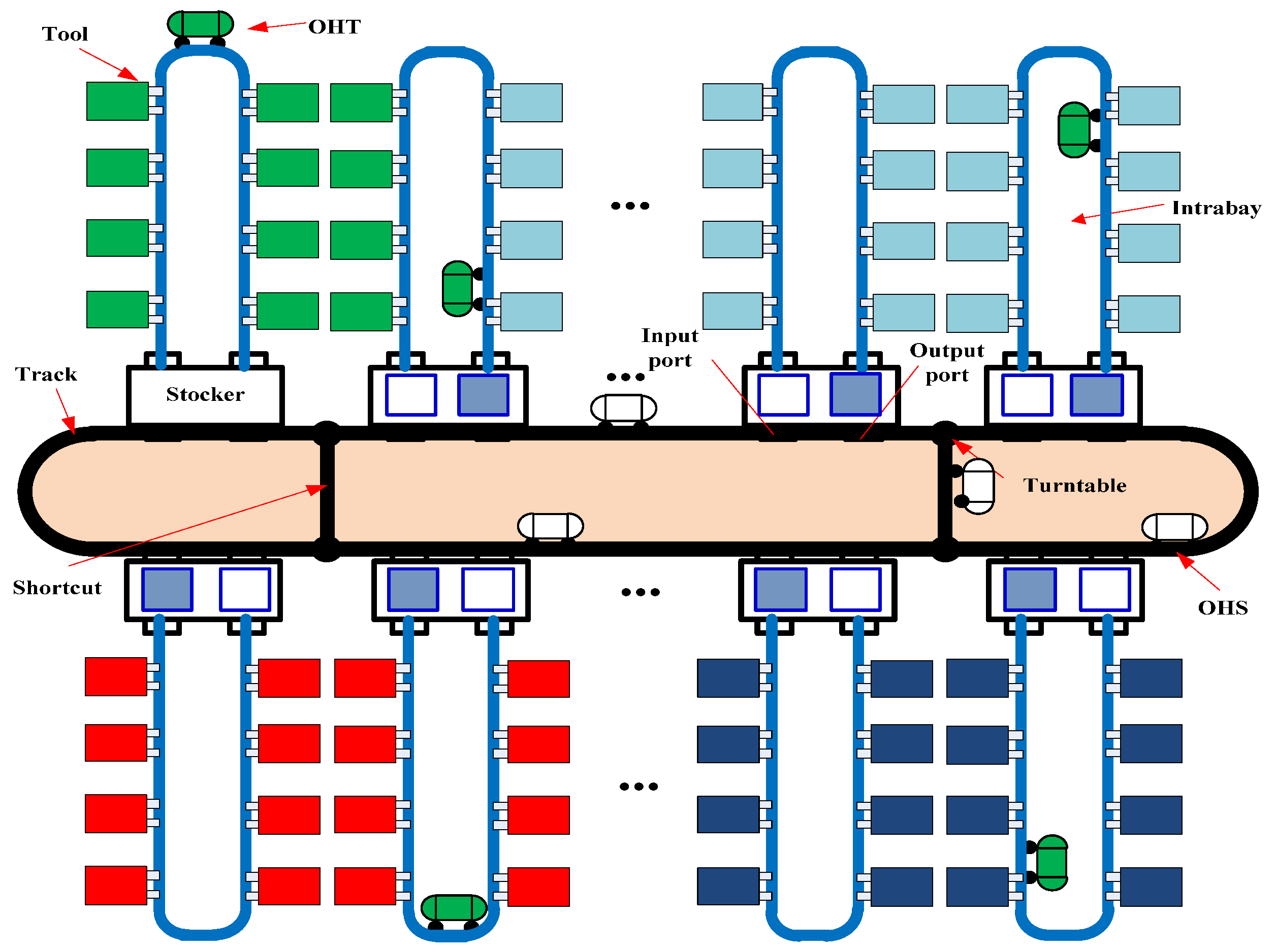
• The distance of the Interbay loop track is 456 m, including 24 Intrabay (workstation) subsystems, five shortcuts, 10 turntables, and 10 OHSs. The length between adjacent stockers is 18 m.
• The speed of OHS remains at 1 m/s.
• A FOUP passes through the turntable for 10 s.
• The OHS vehicle load/unload a FOUP for15 s.
• The process time of cranes in a stocker is assumed to be normally distributed. The mean is 18 s, and the standard deviation (STD) is 5 s.
• The input and output buffer are separated in a stocker. Stockers are assumed with limited capacity. Both input buffer and output buffer capacity are set to be 50.
• A deterministic time interval strategy is used to control the lot feed rate. The feed rate is 1.2 h/lot.
• The simulation time is 1500 h.

4.2. Simulation Results and Discussions

The performance of the proposed algorithm is evaluated by a discrete event model using Arena 14.0, and the dispatching method is programmed with VBA (Visual Basic for Application) embedded in Arena. As mentioned in Section 3.1, when the simulation model meets the reassignment trigger conditions, VBA code of the dispatching method will be called to provide a new optimal assignment to the simulation model.

To verify its performance, some other dispatching rules including traditional fixed weights dispatching rule (FWD) used by Kim et al., and the former rules (Former) are compared with MMDD [31]. The following performance measures are used to evaluate the performance of different dispatching methods: Waiting Time (WT), Transport Time (TT), Throughput (TH), Cycle Time (CT), Vehicle Utilization (VU), and Movement.

In this paper, the influence of vehicle quantity and the feed rates on the material transportation scheduling are considered. Two cases of vehicle quantity are considered: 10 and 12, and two cases of feed rates are considered: 1 lot/per 1.2 h (low load) and 1 lot/per 0.9 h (high load). The total number of experimental scenarios is four. The simulation results are shown in

Table 6. Experimental scenarios 1 (1 lot/1.2 h, OHT = 10).

Dispatching Method	TT (min)		WT (min)		Cycle Time (min)		TH	Movement	VU (%)
	AVG	STD	AVG	STD	AVG	STD
FWD	399.48	1906.14	25.23	588.95	141.32	3873.7	1041	175159	52.29
Former	396.38	1897.47	11.39	110.66	88.07	612.37	1138	182943	54.41
MMDD	398.99	1898.96	10.50	35.49	84.1	308.62	1173	184830	54.94

,

Table 7. Experimental scenarios 2 (1 lot/0.9 h, OHT = 10).

Dispatching Method	TT (min)		WT (min)		Cycle Time (min)		TH	Movement	VU (%)
	AVG	STD	AVG	STD	AVG	STD
FWD	402.53	1926.54	44.6	655.63	225.09	3677.1	1110	182698	54.72
Former	401.47	1959.74	46.73	589.98	210.27	2820.82	1156	194797	58.35
MMDD	399.62	1899.04	23.69	224.59	202.79	2252.09	1206	195977	58.35

,

Table 8. Experimental scenarios 3 (1 lot/1.2 h, OHT = 12).

Dispatching Method	TT (min)		WT (min)		Cycle Time (min)		TH	Movement	VU (%)
	AVG	STD	AVG	STD	AVG	STD
FWD	400.44	2110.25	28.26	714.13	154.8	4758.1	1023	173949	52.26
Former	401.41	1891.27	13.15	129.6	109.18	921.65	1146	184143	54.76
MMDD	397.14	1897.59	10.18	41.98	84.15	240.61	1173	184617	54.87

and

Table 9. Experimental scenarios 4 (1 lot/0.9 h, OHT = 12).

Dispatching Method	TT (min)		WT (min)		Cycle Time (min)		TH	Movement	VU (%)
	AVG	STD	AVG	STD	AVG	STD
FWD	403.14	2048.63	51.28	777.02	221.2	3469.79	1082	183856	55.31
Former	402.73	2200.97	52.49	664.36	208.03	2677.2	1157	194856	58.47
MMDD	397.23	1898.2	23.14	181.02	204.09	2700.5	1192	194485	57.88

. Table 6 and Figure 8 show that MMDD has better performance in CT, TH, Movement, and VU compared with other rules. As for the TT, MMDD shows a slightly longer compared to the Former and FWD.

It is shown that the TT of all scheduling methods increases in experimental scenarios 3 and 4, which differ from the experimental scenarios 1 and 2. This shows that under high load conditions, there is an increased probability of temporary blockage of vehicles. The performance of the scheduling method in experiment scenarios 2 is better than that in experiment scenarios 1, which shows that the MMDD can improve the overall system performance under the high load condition.

For further analysis, an indicator of the comprehensive function $D$ is introduced to realize deeper comparison of various dispatching methods [32].

$$D={\left(\prod _{i=1}^m{d}_i^{w_i}\right)}^{\frac{1}{w}},$$

(31)

If the performance measure must be maximized:

$$d_i=\{\begin{array}{ll}0,& {\mathrm{if}Y}_i{<Y}_{imin}\\ \frac{Y_i-Y_{imax}}{Y_{imax}-Y_{imin}},& {\mathrm{if}Y}_{imin}\le Y_i\le Y_{imax}\\ 1,& {\mathrm{if}Y}_{imax}<Y_i\end{array}$$

(32)

Otherwise, the performance measure must be minimized:

$$d_i=\{\begin{array}{ll}1,& {\mathrm{if}Y}_i{<Y}_{imin}\\ \frac{Y_{imin}-Y_i}{Y_{imax}-Y_{imin}},& {\mathrm{if}Y}_{imin}\le Y_i\le Y_{imax}\\ 0,& {\mathrm{if}Y}_{imax}<Y_i\end{array}$$

(33)

where $Y_{imin}$ and $Y_{imax}$ are the sets of individual performance measure related to the maximum and minimum objectives, $w_i=1$ and $w={\displaystyle \sum }_{i=1}^m{w}_i=1$. The higher the value of $D$, the better the dispatching method. Figure 9 shows the values of comprehensive measure $D$ from different dispatching methods. MMDD has better comprehensive performance than other rules. Furthermore, STD values of MMDD are lower than the values of other dispatching methods in cycle time, WT, and VU, which show that this method is more stable than other rules. The MMDD proposed in this paper is proved to outperform the other methods.

5. Conclusions

In this paper, a dynamic dispatching method based on fuzzy theory is used to dynamically adjust the parameter weights of the wafer lot’s transportation cost model. Compared to previous work, the proposed method is improved in below areas: (1) The AMHS simulation model built in this paper is complicated and more realistic to the real fab. (2) A new rule based on fuzzy theory is used to dynamically adjust the parameter weights of the wafer lot’s transportation cost model, which can meet the demand of real-time and multi-objective optimal scheduling of the interbay system. The rule is extracted from the sample data, which make up for the lack of expert experience. (3) The dynamic dispatching method proposed in this paper reduces waiting time and cycle time. The throughput, vehicle utilization, and movement increase. The comprehensive measure is better than traditional scheduling methods.

After testing our method in the simulation model, the experimental results suggest the proposed method, MMDD, is a better automated vehicle dispatching solution in complex interbay material handling systems. However, there are still some deficiencies. The scheduling of an interbay material handling system is related to the layout of the wafer factory. In this paper, the wafer factory has a single closed-loop spine layout. Further research is needed for systems with more complex layouts. Moreover, it is worth studying on the relationship between wafer processing strategy and material handling system in future work.

References

1. Agrawal, G.K.; Heragu, S.S. A Survey of Automated Material Handling Systems in 300 mm Semiconductor Fabs. IEEE Trans. Semicond. Manuf. 2006, 19, 112–120. [Google Scholar] [CrossRef]
2. Haddadin, M.; Moreno, W. Automated Material Handling Systems: System of Systems Architecture Examination Semiconductor Manufacturing Perspective. In Proceedings of the 32nd Annual SEMI Advanced Semiconductor Manufacturing Conference (ASMC 2021), Milpitas, CA, USA, 10–12 May 2021; pp. 1–6. [Google Scholar] [CrossRef]
3. Wong, H.S.P.; Akarvardar, K.; Antoniadis, D.; Bokor, J.; Hu, C.; King-Liu, T.-J.; Mitra, S.; Plummer, J.D.; Salahuddin, S. A Density Metric for Semiconductor Technology [Point of View]. Proc. IEEE 2020, 108, 478–482. [Google Scholar] [CrossRef]
4. Montoya-Torres, J.R. A literature survey on the design approaches and operational issues of automated wafer-transport systems for wafer fabs. Prod. Plan. Control 2007, 17, 648–663. [Google Scholar] [CrossRef]
5. Yoon, H.J.; Chae, J. Simulation Study for Semiconductor Manufacturing System: Dispatching Policies for a Wafer Test Facility. Sustainability 2019, 11, 1119. [Google Scholar] [CrossRef] [Green Version]
6. Wang, M.-J.J.; Chung, H.C.; Wu, H.C. Evaluating the 300 mm wafer-handling task in semiconductor industry. Int. J. Ind. Ergon. 2004, 34, 459–466. [Google Scholar] [CrossRef]
7. Le-Anh, T.; De Koster, M.B.M. On-line dispatching rules for vehicle-based internal transport systems. Int. J. Prod. Res. 2005, 43, 1711–1728. [Google Scholar] [CrossRef]
8. Yu, Q.; Li, L.; Zhao, H.; Liu, Y.; Lin, K.Y. Evaluation System and Correlation Analysis for Determining the Performance of a Semiconductor Manufacturing System. Complex Syst. Model. Simulation. 2021, 1, 218–231. [Google Scholar] [CrossRef]
9. Yu, Q.Y.; Yang, H.Y.; Lin, K.Y.; Li, L. A self-organized approach for scheduling semiconductor manufacturing systems. J. Intell. Manuf. 2020, 32, 689–706. [Google Scholar] [CrossRef]
10. Huh, J.; Park, I.; Lim, S.; Paeng, B.; Park, J.; Kim, K. Learning to Dispatch Operations with Intentional Delay for Re-Entrant Multiple-Chip Product Assembly Lines. Sustainability 2018, 10, 4123. [Google Scholar] [CrossRef]
11. Pan, C.; Zhang, J.; Qin, W. Real-time OHT Dispatching Mechanism for the Interbay Automated Material Handling System with Shortcuts and Bypasses. Chin. J. Mech. Eng. 2017, 30, 663–675. [Google Scholar] [CrossRef]
12. Li, L.; Min, Z. An efficient adaptive dispatching method for semiconductor wafer fabrication facility. Int. J. Adv. Manuf. Technol. 2016, 84, 315–325. [Google Scholar] [CrossRef]
13. Zhang, J.; Qin, W.; Wu, L.H. A performance analytical model of automated material handling system for semiconductor wafer fabrication system. Int. J. Prod. Res. 2017, 54, 1650–1669. [Google Scholar] [CrossRef]
14. Zhou, Q.; Zhou, B.H. An impending deadlock-free scheduling method in the case of unified automated material handling systems in 300 mm wafer fabrications. J. Intell. Manuf. 2018, 29, 155–164. [Google Scholar] [CrossRef]
15. Huang, C.J.; Chang, K.H.; Lin, J.T. Optimal vehicle allocation for an Automated Materials Handling System using simulation optimisation. Int. J. Prod. Res. 2012, 50, 5734–5746. [Google Scholar] [CrossRef]
16. Gupta, S.; Hasenbein, J.J.; Park, S. Improving scheduling and control of the OHTC controller in wafer fab AMHS systems. Simul. Model. Pract. Theory 2021, 107, 102190. [Google Scholar] [CrossRef]
17. Wang, J.; Zhang, J. Big data analytics for forecasting cycle time in semiconductor wafer fabrication system. Int. J. Prod. Res. 2016, 54, 7231–7244. [Google Scholar] [CrossRef]
18. Lin, J.T.; Wu, C.H.; Huang, C.W. Dynamic vehicle allocation control for automated material handling system in semiconductor manufacturing. Comput. Oper. Res. 2013, 40, 2329–2339. [Google Scholar] [CrossRef]
19. Wang, C.N.; Chen, L.C. The heuristic preemptive dispatching method of material transportation system in 300 mm semiconductor fabrication. J. Intell. Manuf. 2011, 23, 2047–2056. [Google Scholar] [CrossRef]
20. Zhang, J.; Qin, W.; Wu, L.H.; Zhai, W.B. Fuzzy neural network-based rescheduling decision mechanism for semiconductor manufacturing. Comput. Ind. 2014, 65, 1115–1125. [Google Scholar] [CrossRef]
21. Li, L.; Sun, Z.; Zhou, M.C.; Qiao, F. Adaptive Dispatching Rule for Semiconductor Wafer Fabrication Facility. IEEE Trans. Autom. Sci. Eng. 2013, 10, 354–364. [Google Scholar] [CrossRef]
22. Tyan, J.C.; Du, T.C.; Chen, J.C.; Chang, I.H. Multiple response optimization in a fully automated FAB: An integrated tool and vehicle dispatching strategy. Comput. Ind. Eng. 2004, 46, 121–139. [Google Scholar] [CrossRef]
23. Li, L.; Sun, Z.; Ni, J.; Fei, Q. Data-based scheduling framework and adaptive dispatching rule of complex manufacturing systems. Int. J. Adv. Manuf. Technol. 2013, 66, 1891–1905. [Google Scholar] [CrossRef]
24. Qin, W.; Zhang, J.; Sun, Y. Dynamic dispatching for interbay material handling by using modified Hungarian algorithm and fuzzy-logic-based control. Int. J. Adv. Manuf. Technol. 2013, 67, 295–309. [Google Scholar] [CrossRef]
25. Rong, L.; Wang, Z. An algorithm of extracting fuzzy rules directly from numerical examples by using FN-N. In Proceedings of the IEEE International Conference on Systems (CS 1996), Beijing, China, 14–17 October 1996; pp. 1067–1072. [Google Scholar]
26. Qin, W.; Zhang, J.; Sun, Y. Multiple-objective scheduling for interbay AMHS by using genetic-programming-based composite dispatching rules generator. Comput. Ind. 2013, 64, 694–707. [Google Scholar] [CrossRef]
27. Park, T. Effective vehicle dispatching method minimising the blocking and delivery times in automatic material handling systems of 300 mm semiconductor fabrication. Int. J. Prod. Res. 2009, 47, 3997–4011. [Google Scholar]
28. Wu, L.H.; Mok, P.Y.; Zhang, J. An adaptive multi-parameter based dispatching strategy for single-loop interbay material handling systems. Comput. Ind. 2011, 62, 175–186. [Google Scholar] [CrossRef]
29. Yugma, C.; Blue, J.; Dauzère-Pérès, S.; Vialletelle, P. Integration of scheduling and advanced process control in semiconductor manufacturing: Review and outlook. In Proceedings of the IEEE International Conference on Automation Science and Engineering (CASE 2015), Taipei, Taiwan, 18–22 August 2015; pp. 93–98. [Google Scholar]
30. Mittler, M.; Schoemig, A.K. Comparison of dispatching rules for semiconductor manufacturing using large facility models. In Proceedings of the 31st Winter Simulation Conference (WSC 1999), Pheonix, AZ, USA, 5–8 December 1999; pp. 709–713. [Google Scholar]
31. Kim, B.; Shin, J.; Jeong, S.; Koo, J. Effective overhead hoist transport dispatching based on the Hungarian algorithm for a large semiconductor FAB. Int. J. Prod. Res. 2009, 47, 2823–2834. [Google Scholar] [CrossRef]
32. Derringer, G.; Suich, R. Simultaneous Optimization of Several Response Variables. J. Qual. Technol. 1980, 12, 214–219. [Google Scholar] [CrossRef]
Figure 1. Separate Layout Structure Diagram of AMHS.
Sustainability 14 13882 g001
Figure 2. Real-time scheduling process of interbay material handling system.
Sustainability 14 13882 g002
Figure 3. Dynamic dispatching methods scheme of interbay material handling system.
Sustainability 14 13882 g003
Figure 4. The membership function of input variables.
Sustainability 14 13882 g004
Figure 5. The inference process of method based on fuzzy theory.
Sustainability 14 13882 g005
Figure 6. The inference process of fuzzy logic.
Sustainability 14 13882 g006
Figure 7. Process sequence of FOUP A, B, and C (the numbers represent the Bay number).
Sustainability 14 13882 g007
Figure 8. The results of different performance indexes.
Sustainability 14 13882 g008
Figure 9. The values of comprehensive function D values and STD of different performance. (a) Values of D from different dispatching methods; (b) STD of TT from different dispatching methods; (c) STD of WT from different dispatching methods; (d) STD of Cycle time from different dispatching methods.
Sustainability 14 13882 g009