Highlights
What are the main findings?
- No significant impacts of FeCl3 and HCl to the ship’s crew were identified in this assessment.
- For the marine environment, the natural iron levels and variability were found to be much greater than those produced by the hypothetical experiment.
- HCl deposition to the marine environment was found to have no significant impact.
What is the implication of the main finding?
- The hypothetical small-scale field test can possibly be carried out.
Abstract
Various authors have highlighted the possible removal of methane from the atmosphere via oxidation by broad releases of iron salt aerosols in order to serve climate protection goals. This technique is known as enhanced atmospheric methane oxidation (EAMO). This study proposes and employs a modeling approach for the potential environmental impacts associated with a hypothetical small-scale field test of EAMO consisting of seeding cargo-ship exhaust plumes with iron salt aerosols. Using a sample region in the Southern Caribbean Sea as a hypothetical testing site, it provides assessments of potential impacts to air quality, human health, and the marine environment. The modeling focuses on the incremental difference between conducting the hypothetical field test and a no-action scenario. The model results are compared to ambient air standards and pertinent screening thresholds, including those associated with pertinent health risk metrics. The overall loading to the marine environment is contrasted against background rates of iron deposition to the marine surface. No significant impacts were identified in this assessment. The hypothetical atmospheric emissions of both FeCl3 and HCl that the ship’s crew may be exposed to remained below governmental guidance levels. The potential deposition of FeCl3 to the marine environment was found to be very minor in relation to the natural contributions experienced within the Southern Caribbean. Similarly, HCl deposition was assessed for potential impacts to the marine environment but was found to have no significant impact.
1. Introduction
Methane is the second most important greenhouse gas by its radiative forcing and it has a 100-year global warming potential 32 times larger than CO2 [1]. Current warming due to methane is about 0.5 °C while it is about 0.8–0.9 °C for CO2 [2,3] The rise in atmospheric methane has been accelerating in recent years: 2020 and 2021 set new consecutive annual records for the increase in atmospheric levels of methane (respectively, 15.3 ppb and 17 ppb), the largest increase since 1983 when systematic measurements began [4]. In order to avoid about 0.25 °C of additional warming due to methane by 2050 and 0.5 °C by 2100, acting rapidly with mitigation measures is necessary to slow the rate of global-mean warming [3]. If the rise in methane levels continues, it will become very difficult to meet global climate protections goals [5]. Risks due to destabilization and melting of shallow sea methane hydrates are potentially significant [6]. However, because methane is such a large part of climate forcing, it also presents an opportunity for addressing the problem, especially because its atmospheric lifetime is relatively short (about 10–12 years). Although methane control cannot replace the necessity of major reductions in emissions of CO2, significant reductions in the methane burden would ease the timescales required to reach required CO2 reduction targets. Further, methane control could be carried out at a cost that is low relative to the parallel measures being taken to reduce CO2 [5].
The main sink of methane in the troposphere, about 90%, is the hydroxyl radical [7]; the chlorine radical sink is only about 2.5% [8]. However, chlorine radicals react with methane 16 times faster than hydroxyl radicals [9]. FeCl3 generates chlorine atoms catalytically up to 78 times by hour [10] and, consequently, can enhance the natural oxidation of methane. The experiments for generating Cl atoms from iron salt aerosols have been conducted in well-known and controlled laboratory conditions, using a 3 m3 smog chamber test. Their performance in real-world conditions in a marine environment is not yet known.
Various authors have highlighted the possible removal of methane from the atmosphere via oxidation by broad releases of iron salt aerosols [11,12,13]. This technique is labeled here as enhanced atmospheric methane oxidation (EAMO). Before undertaking any such releases, it is vital to understand any potential negative impacts.
The purpose of this paper is to propose a modeling approach for the potential environmental impacts associated with a hypothetical small-scale field test of EAMO consisting of seeding cargo-ship exhaust plumes with iron salt aerosols. Using a sample region in the Southern Caribbean Sea as a hypothetical testing site, it provides assessments of potential impacts to air quality, human health, and the marine environment. This study does not address permitting or regulatory issues, as it only addresses a hypothetical EAMO scenario, nor does it address the potential efficacy of iron salt aerosols. This environmental impact modelling based on a hypothetical field test is a pre-requisite before possibly undertaking open field experiments to evaluate the efficacy of the proposed EAMO method to remove methane from the troposphere.
The next section describes the material and methods used for this environmental impact modelling in separate sections for air quality and the marine environment. Then, the following sections provides the results obtained, a discussion section, and the conclusions.
2. Materials and Methods
2.1. Air Quality
To understand the atmospheric concentrations and rates of particle deposition associated with the field test, we conducted dispersion modeling analyses. Methane Action, a U.S. non-profit group (www.methaneaction.org, accessed on 22 June 2022), provided proposed atmospheric emission rates, chemical composition, and broad source configuration information necessary to set up the dispersion modeling scenario. The methods and results of this atmospheric analysis are described in detail in the following sections.
2.1.1. Environmental Setting
Atmospheric aerosols containing iron are largely emitted from mineral sources and often in windblown dust from deserts, such as contributions of iron from the Sahara Desert in Africa [14]. However, atmospheric iron concentrations are also produced through the combustion of fossil fuels and through biomass combustion. Within the Southern Caribbean study region, the annual mean concentrations of iron particles have been modeled as a range of 0.1 to 1.0 µg/m3 [15]. The size distributions of iron-containing aerosols varies as a function of the source of emission, but a global model from the previously cited study indicates a global average of roughly 2.4 µm with an additional study indicating 4.4 µm [16]. Iron particles emitted from combustion processes start out small but may increase in size over time due to chemical processes (e.g., sulfate formation) or growth through uptake of moisture in the atmosphere. Conversely, iron emitted through processes that include larger particle size bins (e.g., uncontrolled coal combustion or windblown dust events) will undergo rapid loss, or deposition, of those particles through sedimentation.
As discussed in detail in the Marine Environment section, the background iron contributions to the ocean within the Caribbean are influenced by dust blown from the Sahara Desert and, at a more localized scale, from river outflows. This study will use a range of atmospheric particle sizes to assess the potential atmospheric concentrations of iron in contrast to the existing background concentrations and will also estimate the rates at which those particles deposit onto the ocean surface.
2.1.2. Modeling Approach
The purpose of the hypothetical field study is to observe atmospheric chemistry changes that occur when iron aerosols and hydrogen chloride are added to ship exhaust, and to understand how such changes influence ambient methane concentrations. The technical air-dispersion modeling study was developed to simulate near-vessel concentrations, the deposition rates of iron to the marine environment, and any influence of such deposition. The technical approach and modeling parameters are described below.
The hypothetical project location is in the Caribbean Sea and assumes the use of a vessel simulated as the general structure of a cargo ship. The modeled emissions assumed injections of iron (III) chloride (FeCl3) into the plume at a rate of 75–750 g per hour (g/h) and injections of hydrogen chloride (HCl) into the plume at a rate of 7.5–75 kg per hour (kg/h). The particle size of the material injected into the vessel emission stack was assumed to range from 1 µm to 10 µm in aerodynamic diameter. While the authors recognize that the injected particles may be smaller, such smaller particles would be expected to grow due to chemical reactions or uptake of moisture, as discussed previously.
2.1.3. Dispersion Model Selection
The American Meteorological Society (AMS)/United States Environmental Protection Agency (EPA) Regulatory Model Improvement Committee (AERMIC) developed the AMS/EPA Regulatory Model (AERMOD) to perform air-dispersion simulation [17]. There are two input data processors that are regulatory components of the AERMOD modeling system: the AERMOD Meteorological Preprocessor (AERMET), a meteorological data preprocessor that incorporates air dispersion based on planetary boundary-layer turbulence structure and scaling concepts, and the AERMOD Terrain Preprocessor (AERMAP), a terrain data preprocessor that incorporates complex terrain using U.S. Geological Survey (USGS) Digital Elevation Data.
2.1.4. Emission Source Parameter
The hypothetical ship stack was simulated in AERMOD as a point source located at the center of the ship. The emission rates, in grams per second, were used to perform the modeling along with stack and meteorological parameters. The model yields estimated ambient air concentrations and deposition rates. The following modeling parameters were assumed:
- Release Height [18]: 47 m;
- Emission Rate:
- –
- HCl: 75,000 g per hour (20.833 g/s);
- –
- FeCl3: 750 g per hour (0.208 g/s);
- Exit Temperature [19]: 345.0 °C;
- Stack Inside Diameter [17]: 0.5 m;
- Exit Velocity [17]: 25.8 m per second.
Building downwash describes the effect that wind flowing over or around buildings has on plumes released from nearby stacks. Buildings can create an eddy (a cavity of recirculating winds) immediately adjacent to the buildings resulting in elevated near-building concentrations. Assessment of downwash is necessary to make sure all instances of peak concentrations are captured.
Structure downwash was applied within the EPA’s Building Profile Input Program for PRIME (BPIPPRM) to simulate the hypothetical ship structure within AERMOD [20]. Structures implemented into the model include the ship deck, the ship bridge and ship stack. It should be noted that while the ship exhaust plume is expected to behave like the modeled parameters, the actual vessel may have a different physical configuration. The modeled hypothetical ship was a 400-m × 60-m cargo ship, oriented such that the stack observed the highest downwash and produced the most elevated downwind concentrations.
2.1.5. Terrain Data
This analysis assumes a stationary ship located well offshore, so terrain was assumed to be flat without the requirement for elevation data files from the USGS. While, in reality, an EAMO testing vessel would likely be underway at the time of testing, the authors here characterize the most conservative case.
2.1.6. Meteorological Data
With the dispersion modeling occurring offshore, modified treatment of the meteorological data can allow for a more appropriate representation of the meteorological conditions. The EPA has previously approved, for multiple projects, the use of the Coupled Ocean Atmosphere Response Experiment (COARE) air–sea flux procedures for the development of meteorological data [21]. A preprocessor program, AERCOARE, was designed for this preprocessing step. However, the available buoy data did not contain sufficient data to run AERCOARE alone and, instead, a hybrid data set that used both AERCOARE and AERMET was applied.
To make this study realistic, a hypothetical demonstration location was chosen in the Caribbean Sea, in international waters. The wind speed, wind direction, temperature, pressure, and relative humidity from the Eastern Caribbean Sea Buoy (Station 42059) [22] were combined with the other necessary parameters obtained from a sample international airport meteorological station proximate to that buoy (World Meteorological Organization (WMO) Id 78990 [23]. The buoy data was processed as an “onsite” station with the surface meteorological station defined as the airport station. A full set of 5 years of meteorological data was used.
The surface characteristics for the buoy (used in the AERSURFACE pre-processor) were the default albedo, Bowen ratio, and surface roughness length for open water. Upper air data for the AERMET processor were from a sample upper air station located on a proximate island (WMO 78988).
2.1.7. Receptor Grids
Receptors are the specific locations at which concentrations are measured from the air-dispersion modeling. A grid was developed with 20 m spacing for potential crewmember locations across the ship. The receptor grid was designed in the shape of the hypothetical container ship, with a length of 400 m and width of 60 m. Flagpole heights, which represent the height above the surface where concentrations are assessed by the model, were assumed for a deck height of 15 m (rather than ground or sea level) to capture potential crewmember exposure. A second grid was developed with 100 m spacing spanning 10.6 km along the X-axis and 6.4 km along the Y-axis (67.84 km2). The extent of the larger, over-water domain was selected to capture the full plume impact area to capture deposition on the sea. Flagpole heights were not assumed for this grid and, instead, concentrations and depositions were determined at the water surface.
2.1.8. Downwash
Representative structures were entered into the model in order to capture the potential downwash effects on plume dispersion on the emission exhaust stack. The presence of structures (such as the crew accommodations or captain’s deck on a cargo ship) can form localized turbulent zones that can force the plume towards the ground. This is important to consider for potential pollutant impact on crew members and for deposition effects on the marine environment [24].
2.1.9. Iron Deposition Options
Deposition modeling of particles can employ two techniques to calculate cumulative deposition:
- “Method 1” is used when a significant fraction (greater than about 10 percent) of the total particulate mass has a diameter of 10 μm or larger. The particle size distribution must be known reasonably well in order to use Method 1.
- “Method 2” is used when the particle size distribution is not well-known and when a small fraction (less than 10 percent) of the mass is in particles with a diameter of 10 μm or larger. The deposition velocity for Method 2 is given as the weighted average of the deposition velocity for particles in the fine mode (i.e., less than 2.5 μm in diameter) and the deposition velocity for the coarse mode (i.e., greater than 2.5 μm but less than 10 μm in diameter).
Due to the uncertainty in the particle size distribution and the assumption that the particles were less than 10 μm in diameter, this analysis employed Method 2 for three different aerodynamic particle sizes.
The parameters used in Method 2 consist of:
- Particle diameter: This refers to aerodynamic particulate diameter in microns for each particle size category.
- Fine mass fraction: This is the fraction of particles found in the fine mode.
For this analysis, it was assumed that each of the three aerodynamic diameters (1.0, 2.5, and 10.0 μm) were composed of a uniform particle size, thus assigned a value of 1.0.
2.1.10. Gaseous Deposition Options
The EPA’s AERMOD model has added the ability to estimate gas deposition as an “alpha,” or non-regulatory, option that is under evaluation by the agency. To assess the potential deposition of HCl to the marine environment, this option was applied. The option requires additional parameters, including season identification, land use type, diffusivity in air, diffusivity in water, cuticular resistance to uptake by leaves (not applicable here), and Henry’s Law constant [25]. Two configurations of these parameters were considered to provide a range of potential results. Table 1, below, describes each of the physicochemical parameters that were applied. The land use type was assumed to be water and the season was taken to be summer, given the latitude of the proposed study.

Table 1.
Physicochemical properties considered for gas-deposition modeling.
2.1.11. Impact Assessment Approach
The concentration outputs of HCl and iron salts were determined using the modeled concentration value and the most conservative emission rates as well as the conservative assumption that the ship was stationary, discussed above. The maximum 1-h modeled concentration outputs were then compared to the National Institute for Occupational Safety and Health (NIOSH) Reference Exposure Levels (REL), which is 5 parts per million (ppm) or 7 milligrams per cubic meter (mg/m3), not to be exceeded at any time, for HCl [30] and 1 mg/m3, not to be exceed during a 10-hour work period, for iron salts [31].
The maximum 24-hour modeled concentration outputs for iron salts were then compared to the EPA National Ambient Air Quality Standards (NAAQS), which are 150 micrograms per cubic meter (µg/m3) for particulate matter with a diameter of 10 microns or less (PM10) and 35 µg/m3 for particulate matter with a diameter of 2.5 microns or less (PM2.5) [32]. It is assumed that 100% of iron salt concentrations are size PM10 (or smaller).
The REL are used by NIOSH for the occupational exposure limits it recommends for protecting workers from hazardous substances and conditions in the workplace. Therefore, if the modeled concentrations are below the corresponding REL, it can be reasonably concluded that any potentially exposed crewmembers are unlikely to observe adverse health effects.
The NAAQS were designed by the EPA under the U.S. Clean Air Act [33], to establish ambient concentration standards for six criteria pollutants that would be protective of public health. Specifically, for this study, the short-term, 24-hour PM10 and PM2.5 NAAQS were applied for comparison to the modeled dispersion of particulate iron salts. There are annual PM standards that were not applied for this study based on the short-term duration. Similarly, if the modeled concentrations are below the corresponding NAAQS, it can be reasonably concluded that any potentially exposed crewmembers are unlikely to observe adverse health effects.
The off-ship and sea-level area deposition (in grams per square meter, g/m2) of iron salts were obtained as outputs from the AERMOD model. The deposition results were calculated for a range of averaging times (hourly, daily, monthly, annually) and a range of particle sizes to provide the potential range of deposition rates for iron salts on the ocean surface. The results presented are the maximum deposition rates modeled for a month averaging period, as applied to a two-week field-test duration. The maximum modeled daily averaging period results would have been overly conservative for this analysis.
2.2. Marine Environment
The project proposes to assess the feasibility of removing methane from the atmosphere through oxidation using chlorine atoms generated by iron-containing sea salt aerosols. One phase of the project will increase the concentration of iron in a fuel exhaust plume by adding iron salt such as FeCl3. A second project phase will increase iron concentration and also decrease the pH of the exhaust plume by adding dilute HCl. This evaluation assesses the potential effects of increased atmospheric iron and HCl deposition on the near-surface marine environment.
2.2.1. Iron Aerosols
Iron is a very important micronutrient in marine waters which influences the presence of phytoplankton. While iron is an abundant element globally, it is estimated that lack of available iron limits phytoplankton growth in about thirty to fifty percent of open ocean waters, particularly in the high-nutrient low-chlorophyll (HNLC) areas in high-latitude regions [34]. Iron concentrations are typically higher in coastal waters and estuaries where riverine and terrestrial dust inputs are higher. Conversely, iron concentrations are characteristically low in the surface or “photic” zones of the open ocean where phytoplankton algae predominate. As depth increases in deep oceans, iron concentrations tend to increase, which leads to ocean upwelling zones (where currents bring deep ocean waters to the surface) which have higher iron concentrations and correspondingly higher phytoplankton production—a testament to the iron–phytoplankton relationship. However, regions exist where surface-water iron concentrations can be elevated, but the solubility of the iron can be extremely low, limiting the “bioavailability” of the iron to phytoplankton.
The distribution and concentrations of dissolved and particulate iron in the ocean are quite variable in terms of both time and space. Observed iron concentrations are a complex function of spatially and temporally varying atmospheric, terrestrial, and riverine, external inputs; spatial and vertical redistribution by ocean currents biological uptake; recycling within biological systems; deposition to sediments; and other chemical and physical processes which can add or remove iron from the dissolved, biologically available pool [35,36]. Measured dissolved iron concentrations in the ocean range over six orders of magnitude from lows in the surface waters of open ocean HNLC regions to highs in hydrothermal vent fluids, with all other marine environments falling between these extremes.
Iron is generally available for phytoplankton use when it is in an un-oxidized dissolved or colloidal form (as opposed to an oxidized particulate form). Iron limitation in HNLC waters has been demonstrated in experiments where iron addition to surface waters has initiated intense phytoplankton growth or “blooms” [37]. Such blooms occur when changes in nutrient availability alters the relative balance between phytoplankton growth rates and phytoplankton consumption grazing by higher invertebrate and vertebrate trophic levels.
When compared to other nutrients, iron is disproportionately used in metabolic processes as opposed to building biomass. As a result, the addition of iron can promote certain phytoplankton species to bloom and outcompete other species. Phytoplankton species, such as cyanobacteria, that transform nitrogen from atmospheric gas to a plant or bacteria nutrient, require much more cellular iron to support growth than species that use nutrient nitrogen dissolved in ocean water. Certain cyanobacteria (or “blue green algae”) species are associated with harmful algae blooms. These types of blooms are mentioned here to underscore the need for understanding a region’s history of harmful algae blooms or evidence of severe nitrogen limitation in the region’s phytoplankton community.
The Southern Caribbean Sea is not one of the HNLC regions where marine productivity is greatly limited by the supply of iron in the region. The Southern Caribbean receives iron from several sources. The area is downwind of the Saharan Desert and, therefore, experiences a major plume of iron-rich atmospheric dust. Much of this occurs as the entrainment of particles in rainfall (wet deposition) during the summer when the Atlantic intertropical convergence zone (ITCZ) is located over the region resulting in high rainfall. Concentrations of dissolved iron in the coastal ocean, shallow seas overlying the continental shelves, and semi-enclosed basins are typically several orders of magnitude higher than those in the open ocean due to riverine and other inputs. Three large rivers, the Amazon, Orinoco, and Magdalena, discharge up current of or directly into the Southern Caribbean. A major upwelling occurs seasonally in the region bringing iron-rich deep ocean waters to the surface [38]. These three sources, atmospheric, riverine, and upwelling, make the Southern Caribbean less iron limited than other regions.
Modifications to the existing iron loading in the region and any associated change in the phytoplankton balance resulting from the hypothesized field test are key aspects of this analysis. Two points of consideration for this project are:
- Not all forms of iron affect phytoplankton growth equally;
- Various phytoplankton species access and process iron in different ways, so the relative abundance of phytoplankton species can change during iron-induced blooms.
2.2.2. Hydrochloric Acid
The primary effect of HCl on the marine environment in this hypothetical study would be a change in acidity or pH or surface waters. HCl is a “strong” acid meaning it completely dissociates to hydrogen (H+) and chloride (Cl−) ions in water in comparison to weak acids (where some of the atoms remain bound in the original acid compound). As HCl does not exist in bound form in marine waters and the marine water/atmospheric boundary layer, it is usually measured as “non-sea-salt chloride”. Chloride ions are a common component of marine seawater. Sea salt is recognized as the main source of HCl to land and marine surfaces [39]. Ocean acidification effects on phytoplankton communities frequently use HCl to lower pH in experimental conditions because of its ability to lower pH without introducing other compounds [40].
Sanhueza described HCl (derived primarily from natural sources but also from hydrocarbon combustion) as a ubiquitous component of marine rain with depositions generally higher in tropical latitudes [41]. Haskins et al. calculated total land-surface chloride deposition in the eastern United States as declining from 17.4 to 10.4 g/m2.y from 1998 to 2018 [42]. Annual HCl deposition to ocean surfaces is rarely measured, but a significant effort has been invested in monitoring and calculating coastal and oceanic HCl deposition as a result of spacecraft launches from Cape Canaveral, Florida. Various NASA studies found a maximum of 127 g/m2 chloride deposition in localized areas during some launch events [43,44,45]. Maximum depositions of 5.0 to 15.0 g/m2 chloride were more common per launch. Total nearfield chloride depositions of 3400 kg were estimated for typical launches. HCl deposition rates of 0.427 g/m2 over a 4 square mile (10.36 km2) surface area per launch were found to have no significant impact in a Federal Aviation Administration finding of no significant impact (FONSI) document. These deposition rates provide useful baselines against which to assess this proposal.
2.2.3. Environmental Setting
The hypothetical project area is located in the Southern Caribbean Sea proximate to the Eastern Caribbean Sea Buoy (Station 42059). Ocean currents in the area are usually generated by easterly trade winds and include occasional countercurrents and eddies. The Caribbean Current, the main surface circulation in the Caribbean Sea, flows from east to west. Currents in the project area typically flow towards the northwest [46]. As described above, this general area of the Southern Caribbean Sea experiences strong wind-driven coastal upwelling from January to May along the South American continental margin, between Trinidad and Tobago and Barranquilla, Venezuela.
Atmospheric deposition of iron in the hypothetical project area varies significantly depending on seasonal movement of the intertropical convergence zone and variations in the Saharan dust plume. Duce and Tindale estimated atmospheric deposition of iron in the region varied from 100 to 1000 mg/m2·y [47]. Luo et al. [48] modeled atmospheric deposition of soluble iron species at a much finer scale than the Duce and Tindale total iron-deposition estimates. Luo et al. calculated 3 to 16 mg/m2·y of soluble iron deposition in the Netherlands Antilles. Luo et al.’s region deposition patterns closely mirrored the northern extent of the ITCZ in the southeastern Caribbean. The vast majority of atmospheric iron is believed to be deposited in an oxidized particulate form rather than as soluble iron. Therefore, the Duce and Tindale and Luo et al. estimates appear to support each other. However, the much more detailed spatial estimates performed by Luo et al. suggest that the total (as opposed to soluble) atmospheric iron deposition in the region is closer to 1000 mg/m2·y than to 100 mg/m2·y.
2.2.4. Impact Assessment Approach
This assessment focuses on the potential effects of increased atmospheric iron deposition and hydrochloric acid on the near-surface marine environment as the potential driving factor for environmental change that could occur as a result of the hypothesized field test. The assessment compares the estimated mass of substances to be deposited on the ocean surface as a result of the field test with the typical range of substances deposited on the ocean surface at baseline (without the field test).
This impact assessment methodology was developed to analyze potential impacts of a pilot study experiment hypothesis described above. Any efforts to assess larger scale implementation of the EAMO approach should be addressed separately and be performed using the appropriate scale.
3. Results
3.1. Air Quality
The modeled concentration results of the hypothetical field releases are presented in Table 2. Note that the NIOSH REL were converted to match the AERMOD output format of micrograms per cubic meter (μg/m3). As seen in Table 2, modeled 1-h concentrations of HCl and iron salts are below their NIOSH REL and it can be reasonably determined that potential crewmembers would not be exposed to adverse health effects. The 1-hour concentrations for HCl are presented as a conservative maximum acute exposure because there are no 24-h concentrations to compare HCl against.
Table 2.
Dispersion modeling concentrations.
The modeled 24-h concentrations of iron salts are below the NAAQS for PM10 and PM2.5. It can be reasonably determined that potential crewmembers would not be exposed to adverse health effects that are above PM10 or PM2.5 exposure experienced in other professions. For the iron salt concentrations, maximum 1-h concentrations are also presented to give an indication of maximum acute exposures relative to the 24-h concentrations, but there are no regulatory standards to compare the 1-h results against.
The modeled FeCl3 deposition results are presented in Table 3, below. A range of modeled particle sizes are studied to observe the effect of increasing particle in the absence of defined iron salt emission particle size distribution. The amount of iron salts deposited onto the ocean surface increases with time and increased particle size within the confines of the model domain.
Table 3.
FeCl3 deposition modeling results.
The total deposition loading of iron to the marine environment over the two-week study would range from 4.65 kg to 16.28 kg, spread across the 67.84 km2 study area.
The HCl gaseous deposition results are presented in Table 4. The results are presented as a range because AERMOD was used to assess two different physicochemical configurations identified in the literature. Overall, deposition total mass would be expected to be between 4.34 and 5.41 kg over the course of the two-week study across the whole domain.
Table 4.
HCl gaseous deposition results.
Depiction of the FeCl3 and HCl deposition results generated using ESRI’s ArcGIS and U.S. aerial imagery, are provided in Figure 1 and Figure 2, respectively. The wind rose of Figure 3, produced using Python programming libraries, depicts the average conditions of the five years of meteorological data used in the dispersion model.
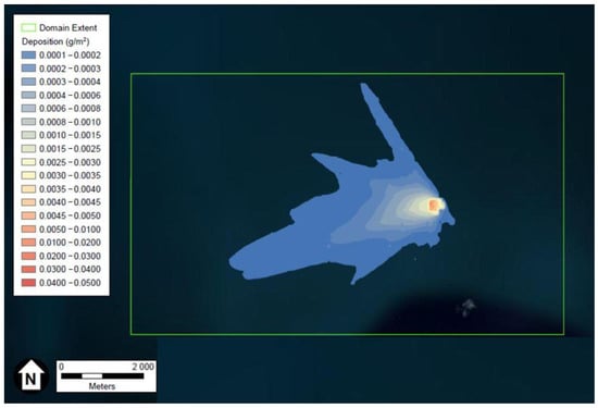
Figure 1.
Depiction of the maximum FeCl3 particles deposition in g/m3 after two weeks. Figure generated using ESRI’s ArcGIS and U.S. aerial imagery.
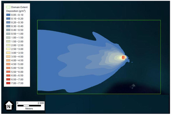
Figure 2.
Depiction of the HCl maximum deposition in g/m3 after two weeks. Figure generated using ESRI’s ArcGIS and U.S. aerial imagery.
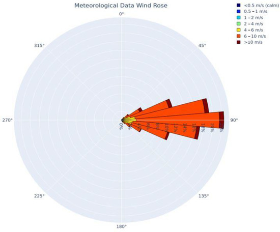
Figure 3.
Wind rose depicting the five years of meteorological data used in the dispersion model, produced using Python programming libraries.
Figure 3 provides a depiction of the frequency of winds by direction and wind speed for all hours that were modeled (the five-year period). The image demonstrates the predominant wind from the east that is pervasive in the eastern Caribbean where the majority of the meteorological data was collected.
3.2. Marine Environment
The field test is assumed, in this study, to run for up to 14 days. The dispersion modeling assessed the impacts of increased atmospheric iron deposition across a modeling region of 10.6 km by 6.4 km (67.8 km2). Total increased atmospheric iron deposition in this area over the 14-day project period is estimated to be between 4.65 to 16.28 kg. This equates to average iron-deposition rate of 0.0046 to 0.016 mg/m2.day. Duce and Tindale’s (1991) 100 to 1000 mg/m2·y baseline total atmospheric iron-deposition rates for the region discussed above equate to 0.27 to 2.74 mg/m2·day. Luo et al.’s modeled soluble iron atmospheric deposition rates for the region equate to 0.01 to 0.04 mg/m2·day. With-project total soluble iron-deposition values were not modeled, but it is assumed the vast majority of project-generated iron deposition would be in particulate form and that the ratio of soluble iron to total iron deposition would be equal to or less than the baseline ratio. These values are compared in Table 5.
Table 5.
Baseline and project-based iron deposition to ocean surface.
Data on monthly or season variation in total atmospheric iron deposition to ocean waters in the region are not available. However, the best regional annual estimates consistently vary by an order of magnitude. It is known that seasonal movement of the ITCZ coupled with seasonal variation in the Saharan dust plume result in large seasonal variations in the daily atmospheric deposition of total nitrogen in the region. Seasonally episodic upwellings coupled with seasonal variation in river flow also produce significant variability in surface seawater water iron concentrations in the South American continental coastal waters. The hypothesized field test would increase total atmospheric iron deposition by 1–2% in a 67.8 km2 area of 1000 to 2500 deep open ocean water. While this is an increase over baseline daily annual average deposition, the with-project condition appears to be within the normal annual variation in atmospheric iron deposition experienced within the study area.
The hypothetical project is predicted to deposit between 4.43 kg and 5.41 kg of HCl in the 67.84 km2 study area over a 14-day period. This equates to a deposition rate of 0.0047 to 0.0057 mg/m2 day and a total deposition of 0.065 to 0.080 mg/m2 for the period. A small area will experience depositions of 2.50 to 7.50 mg/m2 over the entire study period. These 14-day total deposition rates compare favorably with the 5.0 to 15.0 g/m2 nearfield and 0.427 g/m2 total impact area deposition rates described above for Cape Canaveral launches. The comparison is even more favorable when the acceptable Canaveral rates are considered as short term, single-day-or-less events.
Since the seminal paper on ocean acidification was published in 2003, studies of the effect of changing pH on oceanic phytoplankton have been conducted at an ever-increasing rate [49]. Though this new research was not available to the Cape Canaveral studies referenced above, there is little evidence to suggest the hypothesized field test would alter the Cape Canaveral conclusions regarding short-term HCl deposition events. In fact, mesocosm and modeling studies have consistently shifted to increasingly longer time frames (generally well over 14 days) in an effort to fully assess the effect of interspecies competition and predation in response to changes in ocean pH [50,51]. Given these facts and the relatively small amount of HCl the field test would deposit on the ocean surface, it is unlikely such a field test, if carried out, would have any long-term effects on the marine phytoplankton community.
There is little documentation of harmful phytoplankton blooms in the region that might be initiated or exacerbated by a 1–2% increase in total iron deposition over the two-week project period. While harmful algae blooms have been documented in the region, these blooms are with benthic macroalgae [52] or Sargassum macroalgae [53]. The Sargassum blooms are a Caribbean- and Atlantic-wide phenomenon thought to be the result of climate change and increased nutrient (particularly nitrogen) availability [54]. The project in its current location and at its current scale would not be expected to affect either of these two harmful algae blooms issues. Likewise, iron-sensitive cyanobacteria are a contributing source of nitrogen influencing Sargassum blooms [54]. A project of the magnitude assessed here would not likely influence regional Sargassum blooms, however.
4. Discussion
A container vessel the size of the one modelled in this hypothetical experiment consumes about 200 tons/day of fuel [55] containing about 45 parts per million of iron (45 g Fe per 1,000,000 g fuel) [56] and releases SO2 [57] and NOx [58], which will oxidize into sulfuric acid and nitric acid. The amounts of iron emitted are one order of magnitude larger than the ones planned during the hypothetical experiment, while the amounts of acidity [59,60,61] emitted are about three orders of magnitude larger.
The atmospheric-dispersion modelling results demonstrate that the proposed pilot study will result in certain elevated air concentrations, but remain below U.S. exposure standards. The pollutant nearest any exposure standards is the HCl. However, the modelled 1-h concentrations of HCl from the project, for both onboard and overwater scenarios, are well below the 7000 µg/m3 U.S. NIOSH recommended exposure level for a 10-h period or the U.S. Occupational Safety and Health Administration’s (OSHA) 7000 µg/m3 permissible 8-h exposure level for HCl. The modelled 1-h averaging period results in higher values than would be obtained in modelling an 8-h or 10-h averaging period. Moreover, the modelling assumes the highest emissions rates to characterize a conservative scenario and the modelling does not consider any chemical transformations of the HCl, which would potentially reduce overall exposure levels.
For the particulate iron salt aerosols, the results similarly demonstrated that the onboard and over-water exposures would not exceed the corresponding U.S. NIOSH recommend exposure levels.
The marine environmental effects of the hypothetical project would be expected to occur through the mechanism of increased atmospheric iron deposition which was modelled using the AERMOD modelling system. Modelled total iron deposition rates are within the normal seasonal variation observed in the region and HCl rates are below those generated by other short-term, episodic deposition events that are believed to have no impact. Therefore, the project would not be expected to significantly affect the atmospheric or marine environment through the atmospheric deposition of iron or HCl. No significant effects would be foreseeable for marine organisms from the hypothetical field test.
While the form of iron generated by combustion of marine fuels is believed to be relatively soluble and, therefore, bio-available, it is assumed the project will not affect the solubility of atmospheric iron deposits to ocean surface waters and, therefore, the bioavailability of iron in the surface waters of the project area, though no evidence was evaluated regarding varying iron solubility [62].
5. Conclusions
No significant impacts were identified in this assessment of the potential impacts to the atmospheric and marine environments as a result of this hypothetical 14-day EAMO field test in the Southern Caribbean Ocean. The atmospheric emissions of both FeCl3 and HCl that the ship’s crew may be exposed to remained below NIOSH guidance levels and, for particles, below the NAAQS.
The authors assessed the potential deposition of FeCl3 to the marine environment (average iron deposition rate of 0.0046 to 0.016 mg/m2·day) and determined that the rate of contribution to the ocean surface is within the natural contributions experienced within the Southern Caribbean. Similarly, HCl deposition was assessed for potential impacts to the marine environment, but the loading rate (total deposition of 0.065 to 0.080 mg/m2 for the 14-day period) was identified as similar to other short-term events that were found to have no significant impact.
Author Contributions
Conceptualization, P.T.J. and R.d.R.; Data curation, T.M.S.; Formal analysis, T.M.S.; Investigation, T.M.S.; Methodology, T.M.S.; Project administration, P.T.J.; Resources, P.T.J.; Supervision, P.T.J.; Validation, P.T.J. and R.d.R.; Writing—original draft, T.M.S.; Writing—review & editing, P.T.J. and R.d.R. All authors have read and agreed to the published version of the manuscript.
Funding
This study was funded in full by the non-profit US NGO Methane Action; see www.methaneaction.org (accessed on 22 June 2022).
Institutional Review Board Statement
Not applicable.
Informed Consent Statement
Not applicable.
Data Availability Statement
The references section includes links to the pertinent data sets used with the models described on Section 2 “Materials and Methods”. The data that support the findings of this study are available from the corresponding authors upon reasonable request.
Acknowledgments
The authors acknowledge the contributions from Robert Woithe of Environmental Science Associates for his support in developing the marine impacts section. The authors would like to thank the reviewers for their time and very helpful comments and suggestions which have greatly improved our manuscript.
Conflicts of Interest
T.M.S. works for ESA which was funded for this study by Methane Action. R.d.R. is a paid consultant of Methane Action. P.T.J. is a member of Methane Action’s Board of Advisors.
References
- Nisbet, E.G.; Manning, M.; Dlugokencky, E.; Fisher, R.; Lowry, D.; Michel, S.; Myhre, C.L.; Platt, S.M.; Allen, G.; Bousquet, P. Very strong atmospheric methane growth in the 4 years 2014–2017: Implications for the Paris Agreement. Glob. Biogeochem. Cycles 2019, 33, 318–342. [Google Scholar] [CrossRef]
- IPCC. AR6 WG1, Climate Change 2021, The Physical Science Basis—Summary for Policymakers. Available online: https://www.ipcc.ch/report/ar6/wg1/downloads/report/IPCC_AR6_WGI_SPM.pdf (accessed on 11 August 2021).
- Ocko, I.B.; Sun, T.; Shindell, D.; Oppenheimer, M.; Hristov, A.N.; Pacala, S.W.; Mauzerall, D.L.; Xu, Y.; Hamburg, S.P. Acting rapidly to deploy readily available methane mitigation measures by sector can immediately slow global warming. Environ. Res. Lett. 2021, 16, 054042. [Google Scholar] [CrossRef]
- NOAA. Increase in Atmospheric Methane Set Another Record During. 2021. Available online: https://www.noaa.gov/news-release/increase-in-atmospheric-methane-set-another-record-during-2021 (accessed on 4 May 2022).
- Nisbet, E.; Fisher, R.; Lowry, D.; France, J.; Allen, G.; Bakkaloglu, S.; Broderick, T.; Cain, M.; Coleman, M.; Fernandez, J. Methane mitigation: Methods to reduce emissions, on the path to the Paris agreement. Rev. Geophys. 2020, 58, e2019RG000675. [Google Scholar] [CrossRef]
- Englezos, P. Clathrate hydrates. Ind. Eng. Chem. Res. 1993, 32, 1251–1274. [Google Scholar] [CrossRef]
- Kirschke, S.; Bousquet, P.; Ciais, P.; Saunois, M.; Canadell, J.G.; Dlugokencky, E.J.; Bergamaschi, P.; Bergmann, D.; Blake, D.R.; Bruhwiler, L. Three decades of global methane sources and sinks. Nat. Geosci. 2013, 6, 813–823. [Google Scholar] [CrossRef]
- Hossaini, R.; Chipperfield, M.P.; Saiz-Lopez, A.; Fernandez, R.; Monks, S.; Feng, W.; Brauer, P.; Von Glasow, R. A global model of tropospheric chlorine chemistry: Organic versus inorganic sources and impact on methane oxidation. J. Geophys. Res. Atmos. 2016, 121, 14271–214297. [Google Scholar] [CrossRef]
- Atkinson, R.; Arey, J. Atmospheric degradation of volatile organic compounds. Chem. Rev. 2003, 103, 4605–4638. [Google Scholar] [CrossRef]
- Wittmer, J.; Zetzsch, C. Photochemical activation of chlorine by iron-oxide aerosol. J. Atmos. Chem. 2017, 74, 187–204. [Google Scholar] [CrossRef]
- Oeste, F.D.; de Richter, R.; Ming, T.; Caillol, S. Climate engineering by mimicking natural dust climate control: The iron salt aerosol method. Earth Syst. Dyn. 2017, 8, 1–54. [Google Scholar] [CrossRef]
- Ming, T.; de Richter, R.; Oeste, F.D.; Tulip, R.; Caillol, S. A nature-based negative emissions technology able to remove atmospheric methane and other greenhouse gases. Atmos. Pollut. Res. 2021, 12, 101035. [Google Scholar] [CrossRef]
- Jackson, R.; Abernethy, S.; Canadell, J.; Cargnello, M.; Davis, S.; Féron, S.; Fuss, S.; Heyer, A.; Hong, C.; Jones, C.; et al. Atmospheric methane removal: A research agenda. Philos. Trans. R. Soc. A 2021, in press. [CrossRef] [PubMed]
- Abadi, M.S.; Owens, J.D.; Liu, X.; Them, T.R.; Cui, X.; Heavens, N.G.; Soreghan, G.S. Atmospheric dust stimulated marine primary productivity during Earth’s penultimate icehouse. Geology 2020, 48, 247–251. [Google Scholar]
- Wang, R.; Balkanski, Y.; Boucher, O.; Bopp, L.; Chappell, A.; Ciais, P.; Hauglustaine, D.; Peñuelas, J.; Tao, S. Sources, transport and deposition of iron in the global atmosphere. Atmos. Chem. Phys. 2015, 15, 6247–6270. [Google Scholar] [CrossRef]
- Gao, Y.; Marsay, C.M.; Yu, S.; Fan, S.; Mukherjee, P.; Buck, C.S.; Landing, W.M. Particle-size variability of aerosol iron and impact on iron solubility and dry deposition fluxes to the Arctic Ocean. Sci. Rep. 2019, 9, 16653. [Google Scholar] [CrossRef]
- AERMOD. The American Meteorological Society (AMS)—Environmental Protection Agency (EPA) Regulatory Model. 2006. Available online: https://www.epa.gov/scram/air-quality-dispersion-modeling-preferred-and-recommended-models#aermod (accessed on 18 July 2022).
- POS. Port of Seattle, Alliance NS. Terminal 5 Cargo Wharf Rehabilitation, Berth Deepening, and Improvements Final Environmental Impact Statement Volume II. 2016. Available online: https://www.portseattle.org/sites/default/files/2018-12/FEIS%20T5%20Volume%20II.pdf 2016 (accessed on 18 July 2022).
- SCG. Starcrest Consulting Group. Port of Los Angeles, Port of Los Angeles Baseline Air Emissions Inventory. 2005. Available online: https://kentico.portoflosangeles.org/getmedia/e9147367-eac0-4cc3-add7-6bfb6123f7e0/REPORT_Final_BAEI (accessed on 18 July 2022).
- EPA (Environmental Protection Agency); Building Profile Input Program (BPIP). 2004. Available online: https://www.epa.gov/scram/air-quality-dispersion-modeling-related-model-support-programs#bpip (accessed on 18 July 2022).
- EPA (Environmental Protection Agency). AERMOD Coupled Ocean Atmosphere Response Experiment (AERCOARE). 2011. Available online: https://www.epa.gov/scram/air-quality-dispersion-modeling-related-model-support-programs#aercoare (accessed on 18 July 2022).
- NOAA. National Data Buoy Center, Station 42059. 2022. Available online: https://www.ndbc.noaa.gov/station_page.php?station=42059&unit=M&tz=EGT (accessed on 30 September 2022).
- NOAA. Global Hourly Integrated Surface Database, WMO Station 78990. 2022. Available online: https://www.ncei.noaa.gov/data/global-hourly/access/ (accessed on 30 June 2022).
- Villalvazo, L.; Davila, E.; Reed, G. Guidance for Air Dispersion Modeling. San Joaquin Valley Air Pollution Control District. 2007. Available online: http://www.valleyair.org/busind/pto/tox_resources/modeling%20guidance%20w_o%20pic.pdf (accessed on 18 July 2022).
- EPA. Environmental Protection Agency. User’s Guide for the AMS/EPA Regulatory Model (AERMOD). 2021. Available online: https://gaftp.epa.gov/Air/aqmg/SCRAM/models/preferred/aermod/aermod_userguide.pdf (accessed on 18 July 2022).
- Wesely, M.L.; Doskey, P.V.; Shannon, J. Deposition Parameterizations for the Industrial Source Complex (ISC3) Model; Argonne National Lab. (ANL): Argonne, IL, USA, 2002. Available online: https://publications.anl.gov/anlpubs/2008/11/62977.pdf (accessed on 18 July 2022).
- Lange, N.A.; Dean, J.A. Lange’s Handbook of Chemistry; McGraw-Hill Education: New York, NY, USA, 1992. [Google Scholar]
- Seader, J.D.; Henley, E.J.; Roper, D.K. Separation Process Principles—Chemical and Biochemical Operations, 3rd ed.; Wiley: New York, NY, USA, 2012; ISBN 978-0-470-48183-7. [Google Scholar]
- The Engineering Toolbox. Gases Solved in Water—Diffusion Coefficients. Available online: https://www.engineeringtoolbox.com/diffusion-coefficients-d_1404.html (accessed on 2 October 2021).
- NIOSH (National Institute for Occupational Safety & Health). CDC—NIOSH Pocket Guide to Chemical Hazards—Hydrogen Chloride. Pocket Guide to Chemical Hazards. 2019. Available online: https://www.cdc.gov/niosh/npg/npgd0332.html (accessed on 18 July 2022).
- NIOSH (National Institute for Occupational Safety & Health). CDC—NIOSH Pocket Guide to Chemical Hazards—Iron Salts (Soluble, as Fe). Pocket Guide to Chemical Hazards. 2019. Available online: https://www.cdc.gov/niosh/npg/npgd0346.html (accessed on 18 July 2022).
- EPA (Environmental Protection Agency). National Ambient Air Quality Standards NAAQS Table. 1990. Available online: https://www.epa.gov/criteria-air-pollutants/naaqs-table (accessed on 18 July 2022).
- EPA (Environmental Protection Agency). Clean Air Act, United States Code 42 U.S.C. § 7401. 1990. Available online: https://www.epa.gov/laws-regulations/summary-clean-air-act (accessed on 18 July 2022).
- Hogle, S.L.; Dupont, C.L.; Hopkinson, B.M.; King, A.L.; Buck, K.N.; Roe, K.L.; Stuart, R.K.; Allen, A.E.; Mann, E.L.; Johnson, Z.I. Pervasive iron limitation at subsurface chlorophyll maxima of the California Current. Proc. Natl. Acad. Sci. USA 2018, 115, 13300–13305. [Google Scholar] [CrossRef]
- Street, J.H.; Paytan, A. Iron, phytoplankton growth, and the carbon cycle. In Metal Ions in Biological Systems; CRC Press: Boca Raton, FL, USA, 2005; pp. 153–193. [Google Scholar]
- Sutak, R.; Camadro, J.-M.; Lesuisse, E. Iron uptake mechanisms in marine phytoplankton. Front. Microbiol. 2020, 11, 566691. [Google Scholar] [CrossRef]
- Boyd, P.W.; Jickells, T.; Law, C.; Blain, S.; Boyle, E.; Buesseler, K.; Coale, K.; Cullen, J.; De Baar, H.J.; Follows, M. Mesoscale iron enrichment experiments 1993-2005: Synthesis and future directions. Science 2007, 315, 612–617. [Google Scholar] [CrossRef]
- Rueda-Roa, D.T.; Muller-Karger, F.E. The southern Caribbean upwelling system: Sea surface temperature, wind forcing and chlorophyll concentration patterns. Deep Sea Res. Part I Oceanogr. Res. Pap. 2013, 78, 102–114. [Google Scholar] [CrossRef]
- Symonds, R.B.; Rose, W.I.; Reed, M.H. Contribution of C1-and F-bearing gases to the atmosphere by volcanoes. Nature 1988, 334, 415–418. [Google Scholar] [CrossRef]
- Osma, N.; Latorre-Melín, L.; Jacob, B.; Contreras, P.Y.; von Dassow, P.; Vargas, C.A. Response of phytoplankton assemblages from naturally acidic coastal ecosystems to elevated pCO2. Front. Mar. Sci. 2020, 7, 323. [Google Scholar] [CrossRef]
- Sanhueza, E. Hydrochloric acid from chlorocarbons: A significant global source of background rain acidity. Tellus B 2001, 53, 122–132. [Google Scholar] [CrossRef]
- Haskins, J.D.; Jaeglé, L.; Thornton, J.A. Significant decrease in wet deposition of anthropogenic chloride across the eastern United States, 1998–2018. Geophys. Res. Lett. 2020, 47, e2020GL090195. [Google Scholar] [CrossRef]
- Dreschel, T.W.; Hall, C.R. Quantification of hydrochloric acid and particulate deposition resulting from space shuttle launches at John F. Kennedy Space Center, Florida, USA. Environ. Manag. 1990, 14, 501–507. [Google Scholar] [CrossRef]
- Schmalzer, P.; Hall, C.; Hinkle, C.; Duncan, B.; Knott, W.; Summerfield, B. Environmental Monitoring of Space Shuttle Launches at Kennedy Space Center-The First Ten Years. In Proceedings of the 31st Aerospace Sciences Meeting, Reno, NV, USA, 11–14 January 1993; p. 303. Available online: https://arc.aiaa.org/doi/abs/10.2514/6.1993-303 (accessed on 18 July 2022).
- FAA. United States Federal Aviation Administration. Environmental Assessment for Space Florida Launch Site Operator License at Launch Complex-46. 2008. Available online: https://www.faa.gov/about/office_org/headquarters_offices/ast/media/sept%202008%20space%20florida%20ea%20and%20fonsi.pdf (accessed on 18 July 2022).
- Govers, L.L.; Lamers, L.P.; Bouma, T.J.; Eygensteyn, J.; de Brouwer, J.H.; Hendriks, A.J.; Huijbers, C.M.; van Katwijk, M.M. Seagrasses as indicators for coastal trace metal pollution: A global meta-analysis serving as a benchmark, and a Caribbean case study. Environ. Pollut. 2014, 195, 210–217. [Google Scholar] [CrossRef] [PubMed]
- Duce, R.A.; Tindale, N.W. Atmospheric transport of iron and its deposition in the ocean. Limnol. Oceanogr. 1991, 36, 1715–1726. [Google Scholar] [CrossRef]
- Luo, C.; Mahowald, N.; Bond, T.; Chuang, P.; Artaxo, P.; Siefert, R.; Chen, Y.; Schauer, J. Combustion iron distribution and deposition. Glob. Biogeochem. Cycles 2008, 22, GB1012. [Google Scholar] [CrossRef]
- Caldeira, K.; Wickett, M.E. Anthropogenic carbon and ocean pH. Nature 2003, 425, 365. [Google Scholar] [CrossRef]
- Hyun, B.; Kim, J.-M.; Jang, P.-G.; Jang, M.-C.; Choi, K.-H.; Lee, K.; Yang, E.J.; Noh, J.H.; Shin, K. The effects of ocean acidification and warming on growth of a natural community of coastal phytoplankton. J. Mar. Sci. Eng. 2020, 8, 821. [Google Scholar] [CrossRef]
- Henson, S.A.; Cael, B.; Allen, S.R.; Dutkiewicz, S. Future phytoplankton diversity in a changing climate. Nat. Commun. 2021, 12, 5372. [Google Scholar] [CrossRef]
- De Bakker, D.M.; Van Duyl, F.C.; Bak, R.P.; Nugues, M.M.; Nieuwland, G.; Meesters, E.H. 40 Years of benthic community change on the Caribbean reefs of Curaçao and Bonaire: The rise of slimy cyanobacterial mats. Coral Reefs 2017, 36, 355–367. [Google Scholar] [CrossRef]
- Tjiong, W. Mapping Sargassum on Beaches and Coastal Waters of Bonaire Using Sentinel-2 Imagery. 2020. Available online: https://edepot.wur.nl/532436 (accessed on 18 July 2022).
- Lapointe, B.; Brewton, R.; Herren, L.; Wang, M.; Hu, C.; Mcgillicuddy, D.; Lindell, S.; Hernandez, F.; Morton, P. Nutrient content and stoichiometry of pelagic Sargassum reflects increasing nitrogen availability in the Atlantic Basin. Nat. Commun. 2021, 12, 3060. [Google Scholar] [CrossRef] [PubMed]
- Notteboom, T.; Cariou, P. Fuel surcharge practices of container shipping lines: Is it about cost recovery or revenue making. In Proceedings of the 2009 International Association Of Maritime Economists (IAME) Conference; IAME: Copenhagen, Denmark, 2009; pp. 24–26. [Google Scholar]
- Ito, A. Global modeling study of potentially bioavailable iron input from shipboard aerosol sources to the ocean. Glob. Biogeochem. Cycles 2013, 27, 1–10. [Google Scholar] [CrossRef]
- IMO (International Maritime Organization). IMO 2020—Cutting Sulphur Oxide Emissions. Available online: https://www.imo.org/en/MediaCentre/HotTopics/Pages/Sulphur-2020.aspx (accessed on 16 June 2022).
- De Lauretis, R.; Ntziachristos, L.T. Carlo EMEP/EEA Air Pollutant Emission Inventory Guidebook. 2019. Available online: https://www.eea.europa.eu/publications/emep-eea-guidebook-2019/part-b-sectoral-guidance-chapters/1-energy/1-a-combustion/1-a-3-d-navigation (accessed on 14 October 2022).
- Sarin, M.; Kumar, A.; Srinivas, B.; Sudheer, A.; Rastogi, N. Anthropogenic sulphate aerosols and large Cl-deficit in marine atmospheric boundary layer of tropical Bay of Bengal. J. Atmos. Chem. 2010, 66, 1. [Google Scholar] [CrossRef]
- Pósfai, M.; Anderson, J.R.; Buseck, P.R.; Sievering, H. Compositional variations of sea-salt-mode aerosol particles from the North Atlantic. J. Geophys. Res. Atmos. 1995, 100, 23063–23074. [Google Scholar] [CrossRef]
- Li, W.; Shao, L.; Wang, Z.; Shen, R.; Yang, S.; Tang, U. Size, composition, and mixing state of individual aerosol particles in a South China coastal city. J. Environ. Sci. 2010, 22, 561–569. [Google Scholar] [CrossRef]
- Kurisu, M.; Sakata, K.; Uematsu, M.; Ito, A.; Takahashi, Y. Contribution of combustion Fe in marine aerosols over the northwestern Pacific estimated by Fe stable isotope ratios. Atmos. Chem. Phys. 2021, 21, 16027–16050. [Google Scholar] [CrossRef]


Publisher’s Note: MDPI stays neutral with regard to jurisdictional claims in published maps and institutional affiliations. |
© 2022 by the authors. Licensee MDPI, Basel, Switzerland. This article is an open access article distributed under the terms and conditions of the Creative Commons Attribution (CC BY) license (https://creativecommons.org/licenses/by/4.0/).