Does Urban Agglomeration Promote the Development of Cities? An Empirical Analysis Based on Spatial Econometrics

Abstract

Based on the panel data of 278 cities in China from 2010–2019, this paper uses the spatial Durbin model to investigate the effect of urban agglomeration on urban economic development under the distance factor. The results show that the impact of urban agglomeration on urban development is sensitive to geographic distance. A moderate geospatial scale can help cities overcome scale deficiencies and the problem of overcrowding. The spillover effect of urban agglomeration is no longer limited to geographical proximity, showing an inverted U-shaped curve with the expansion of distance. It also exhibits heterogeneity across different regions, and integrated development reinforces the positive impact of agglomeration spillovers. The economic distance moderation effect and the core-periphery structure suggest that the direction of spatial interaction is more reflected between high-ranking cites and low-ranking cities, while cities with similar development levels show competitive effects. Specialized agglomeration and diversified agglomeration have differential influences on urban growth. From the perspective of network externalities, the spillover effect of urban agglomeration increases significantly with the expansion of spatial scale, which is distinct from the results using geographical distance.

1. Introduction

Currently, the urbanization rate of China’s permanent population has exceeded 64.72%. The urbanization development is gradually shifting from high-speed growth to high-quality development. The trend of concentration of economic activities has been further strengthened. Urban agglomerations centered on large cities have become important spatial carriers of economic development and the cornerstones supporting economic growth. Along with the continuous advancement of urbanization and industrialization, the direction of regional economic development has gradually changed from the traditional administrative district economy to the urban agglomeration economy, especially the Beijing-Tianjin-Hebei, Yangtze River Delta, Pearl River Delta, and other urban agglomerations have become crucial support for China’s economic development. In early research, the debate on China’s urbanization was more about whether China should choose to continue to follow the expansion path of large cities or the simultaneous growth model of small- and medium-sized cities, facing the problem of choosing the path of agglomeration. In fact, promoting the coordinated development of large, medium, and small cities, and the formation of a spatial pattern of urbanization with coherence, division of labor, and complete functions is the focus of future work. Promoting urbanization development as an important channel for cultivating urban agglomeration areas is also an effective channel for transforming the development mode of large cities and encouraging the coordinated development of small- and medium-sized cities. Along with the construction of the high-speed railway network, the revolution of communication technology, and the advancement of the industrial division of labor among cities, cross-regional development has made urban network increasingly prominent, and the spatial spillover effect has also played an increasingly prominent role in the process of regional economic growth. The development of modern cities also relies more on the interconnection between cities and the optimization of the spatial structure of cities to full exploit agglomeration advantages. The spatial distribution of urban population and factors reflects the spatial connection and structure of cities and has significant differences in economic performance at different geographic scales [1]. Regional development, the formation of metropolitan areas, and urban agglomerations all have their own rules. Defining a reasonable spatial scope and forming effective personnel interflow and economic connections within the appropriate areas is the key to exerting the spillover effect of urban agglomeration.

The same goal of economic growth in different cities will inevitably lead to significant differences in the capacity and results of production factor agglomeration among cities. Cities that benefit from institutional dividends or corresponding resource allocation advantages will inevitably rise rapidly in the agglomeration process, strengthening or altering the original regional spatial agglomeration outcomes. As a result, the economic growth path of the region evolves in a different direction of polarization or diffusion. For this reason, it is necessary to understand whether the process of urban agglomeration in China is promoting or detrimental to urban development and whether the impact is the same for all cities. Moreover, urban development policies with spatial linkages are more significant considering the interactions between cities and the spillover effects generated by agglomeration.

In general, there are few empirical studies about the effects of urban agglomeration on urban economic development, and the role of geographic factors remains not explored effectively. Based on a valid measure of the degree of urban agglomeration, this paper investigates the contribution of urban agglomeration to regional growth and the spillover effects. The possible innovations are as follows. Firstly, the role of urban agglomeration in urban development is explored based on geographic sensitivity, which is rarely investigated in related research. Considering the inconsistent findings when discussing the relationship between urban agglomeration and economic development regardless of spatial scale [2], distance is included in the measurement of agglomeration, taking into account both scale and location perspectives. Secondly, some studies regard the high speed railway opening or urban agglomeration as a regional economic policy to investigate the impact of agglomeration on urban development [3,4,5,6], while others develop agglomeration indicators to examine their impact on the city itself [7,8,9]. These studies ignore urban linkages and spillover effects. In fact, the expanded spatial scope of agglomeration impact, the existence of borrowed size, and the spillover effect of agglomeration all play an influential role in the regional development process [10,11,12]. In this context, this study investigates the spillover effects of urban agglomeration at diverse spatial scales and constructs spatial matrices based on economic distance and urban systems to provide new explanations for the spillover effects of urban agglomeration and lead to novel results. Thirdly, the study compares the disparity in urban agglomeration for urban performance from different perspectives. The research on urban network externalities receives increasing attention from scholars [13,14,15], and the growth effect of urban agglomeration is further analyzed from the industrial agglomeration perspective and the network externality perspective.

2. Literature Review

2.1. The Impact of Urban Agglomeration on Economic Growth

Agglomeration is the tendency of economic activities to concentrate in a geographic space, mainly in the form of industrial clusters or interdependent economic networks formed by the concentration of the same or complementary industries in a specific, adjacent geographic location. The existence of agglomeration results from the additional benefits of input-output linkages, labor sharing, domestic market effects, and knowledge spillovers associated with the expansion of scale that occurs when economic activities are clustered in the same area, that is, agglomeration externalities [16,17,18,19]. In order to obtain further agglomeration economies, cities continue to expand in size, and when they reach the corresponding critical point, agglomeration diseconomies such as environmental degradation, congestion, and increased labor costs begin to emerge. From a single city perspective, urban development accompanied by scale expansion always experiences agglomeration economies and agglomeration diseconomies. In addition, there is an optimal scale that the externalities of agglomeration can be effectively exploited in this state. In earlier studies, agglomeration externalities were defined as being geographically constrained. It was assumed that economic activities outside the region have no impact on the region [20]. The examination of agglomeration externalities has focused more on the ability of industrial diversification or specialization to promote urban growth [21,22] and the input sharing, factor matching, and learning mechanisms required for agglomeration externalities to occur [17]. However, under the trend of economic globalization and regional integration, cities are not isolated islands. The agglomeration of economic activities promotes the development of geographically adjacent areas to form contiguous urban agglomerations gradually. Most cities are more or less connected to the surrounding areas to a certain extent [23]. The cities in the region are increasingly interconnected to form a broader economic unit and a complete urban network system. As the agglomeration externalities of large cities are not limited to the inner city, they have a significant impact on the surrounding areas. Small- and medium-sized cities in the region can also share the agglomeration economy and the radiation effects of the core cities to promote urban growth [24]. The new economic geography emphasizes the influence of agglomeration externalities on regional economic growth within a large geographic range, which makes cities no longer isolated within a certain spatial area, but closely related to neighboring regions. Therefore, when considering the interaction between cities, it is clear that examining the agglomeration effects of a single city is not effective in defining the optimal degree of urban agglomeration. It is more important to study the overall situation and interconnection of cities than the agglomeration economy of an individual city.

2.2. Geographical Factors and Agglomeration Externalities

As one of the important factors affecting regional economic development, the impact of agglomeration economies is considered an economic externality, which arises from the co-location of economic agents. In early studies, due to the neglect of inter-city interactions, agglomeration economies are geographically constrained and have no spillover effects outside the region [13,20]. Subsequently, several researchers have examined agglomeration externalities using spatial econometric methods [25], confirming the required geographical proximity basis, especially the accessibility to major cities and geographic isolation. A large number of empirical studies have proven that agglomeration externalities are highly sensitive to geographic factors, and the effects usually decrease with distance expansion and there are distinct geographic boundaries [20,26]. However, there is also evidence of agglomeration externalities extending to distant regions [27,28]. In general, the closer to the big city, the more conducive it is to capture the spillover effects of agglomeration.

In fact, the net effect of inter-city interaction is the result of urban agglomeration economies and agglomeration diseconomies, and geographical distance plays an important role. Therefore, when examining the economic spillover effects of urban agglomeration on surrounding areas, an appropriate geographic scale should be selected to enhance the reliability of the conclusions [29]. With the rapid development of regional systems, thanks to the construction of transportation infrastructure and information technology innovations, cities and the internal enterprises are benefiting not only from local interactions but also from extra-urban regions, and spatial factors are crucial in reshaping urban growth [30]. The increasing division of labor and economic linkages between cities in the region makes agglomeration externalities break the precondition of geographical proximity, making the distance factor less important [31].

Agglomeration externalities across geographic boundaries have developed rapidly and are no longer restricted to administrative regions. Not only can neighboring cities share agglomeration externalities to gain opportunities for rapid development, but non-adjacent cities can also interact with each other through their connections. When agglomeration externalities are no longer confined to the nodes or adjacent areas of cities, but spill over to larger geographic distances, the scope of agglomeration externalities is expanded. Borrowed size and the emergence of urban network externalities further contribute to the interpretation and enrichment of agglomeration theories and phenomena [32,33,34]. The existence of the spatial competition effect makes it possible for large cities to inhibit the development of small- and medium-sized cities, resulting in agglomeration shadows [13,35]. After considering the spatial connections between cities, the impact of cities and their embedded urban networks on urban economic performance even exceeds their own functions and characteristics [23]. In addition, with the construction of the high-speed railway networks, mechanisms such as matching, sharing, and learning are not strict to specific regions and can exert impact at a larger geographic scope [26]. Long-distance cities can also achieve win-win cooperation through urban networks, and the role of local agglomeration economies is gradually complemented by urban network externalities across geographic boundaries [36,37]. Although urban network structure does not completely replace geographical proximity [36,38], the rise of urban network externalities has led to growing awareness of the expanding geographical expansion of agglomeration externalities [39,40].

2.3. Empirical Research of Urban Agglomeration on Economic Growth

Regional economic development not only depends on its factor input but also has a significant relationship with economic activities in surrounding areas, especially the core cities, whose economic activity has a profound impact on surrounding small- and medium-sized cities [5]. Furthermore, urban growth is even more associated with the joint effect of distance to major cities and agglomeration [41]. The “backwash-diffusion”, “polarization-trickle-down”, and “core-periphery” theories all emphasize the dual effects of agglomeration and diffusion of large cities on surrounding areas. According to the development stages and the location characteristic of the cities, the spillover effects of urban agglomeration will have heterogeneous performance.

The siphoning effect of large cities in the early stage of development will inhibit the growth of small cities, which can only be avoided if the distance from large cities exceeds a certain threshold [35], while the spillover effect of well-developed large cities supports smaller cities gaining stronger growth momentum. Empirical studies have shown that central cities may either have positive spillover effects on adjacent areas or inhibit their growth through competition [42,43,44]. Research based on prefecture-level cities in China confirms that the economic development of small- and medium-sized cities benefits from the spillover effect of agglomeration in large cities and exhibits regional heterogeneity [45]. The spillover effects of different types of large cities on small cities also exhibit heterogeneity. Compared with general prefecture-level cities, the spillover effect of sub-provincial cities is stronger [46].

From the perspective of the urban structure system and location characteristics, empirical studies based on several regions have confirmed that urban agglomeration significantly promotes urban growth in peripheral areas, while hindering urban development in core areas [47,48,49]. In addition, the size of the effect may vary with the distance in a nonlinear relationship because of the different positions of cities in the urban system. Urban agglomeration in peripheral areas helps to increase density and thus enhance human interaction, while in core areas, agglomeration intensifies the intensity of competition between workers and investors [48]. Based on studies in China, it is consistently concluded that urban agglomeration has a stronger promotion effect on regions with relatively low agglomeration and relatively low development [7]. More specifically, research shows that the positive effects of specialization agglomeration are more prominent in less developed inland cities or small cities, while the promotion effect of diversification agglomeration is stronger in developed or coastal cities [50].

In the region-specific research, scholars use the Yangtze River Economic Zone as the sample to find that urban agglomeration helps to improve the quality of economic development [4]. Empirical studies of different urban agglomerations in China indicate that there is still much potential for improving agglomeration externalities in Chinese urban agglomerations [9]. Urban agglomerations that are more agglomerated or have multiple central cities will boast a stronger engine of economic growth. The research further confirms that the impact of urban agglomerations on regional growth is closely related to the spatial distance and the economic development status of the core cities [5,8].

Research on the subject has been mostly restricted to geographic scales that are comparatively easy to measure, such as within regions or urban agglomerations. Although a few previous studies have considered geographic distance in calculating urban agglomeration, little is known about how geographic distance affects the growth effects of agglomeration. In addition, more attention is paid to the role of agglomeration on local growth in the studies of quantifying urban agglomeration on regional development, and spatial spillover effects are usually ignored. The spillover effects of urban agglomeration on urban development and the spatial correlation of urban growth are important for understanding the mechanisms of urban economic growth. This paper supplements the spatial perspective to explore in depth the spatial characteristics of the impact of urban agglomeration.

3. Models and Methods

3.1. Measure the Degree of Urban Agglomeration

Urban economic growth is not only the process of factors agglomeration but also the result of the mutual evolution of the institutional environment and geographic location. Urban agglomeration is usually measured from the perspectives of scale and density, including population size and employment density. However, this method does not reflect the spatial location characteristics of cities. Considering the influence of geographical location, the ratio of urban spatial isolation IS to remoteness IR is used to measure the urban agglomeration situation. On the one hand, the total population of the target city within a certain spatial area is calculated. On the other hand, consider the distance between the city and the core city, measuring its spatial location characteristics of it in the region. The urban agglomeration index calculated using the above method has high values in densely populated areas or areas close to the core city, while it has low values in small cities or areas far from the core city. This index can reflect the spatial location characteristics of the region to a certain extent and measure the urban agglomeration more scientifically by adjusting the size with the relative distance between cities.

$$I{C}_i=IS/IR=Ln({\displaystyle \sum _{j=1}^n{P}_j/I{R}_{ik})}$$

(1)

where IS means the aggregated population in a certain range of the city, $P_j$ is the population size of city j located within the commuting range from city i, and IR is the remoteness of the city i, measured by distance between the city i and the nearest core city k.

The selection of the core city and the determination of the spatial distance are crucial to calculate the urban agglomeration. According to Portnov and Schwartz [48] and Huang et al. [51], the core cities are selected from the perspectives of population size and economic development. First, the population size of districts under city is more than 1.5 million. Second, the GDP of the core city should rank as two of the top in its province. To avoid errors caused by data from a particular year, the average population and GDP data from 2010 to 2019 are used. Based on the selection criteria of core cities, it identified 39 cities as core cities. Due to the sensitivity of agglomeration externalities to distance, combined with the current status of the distance between cities in China, 150 km was used as the benchmark distance, and 25 km is used as the distance increment. Because the average value of the shortest distance from each city to the core city is 165 km, and the median distance is 150.4 km. The distance between cities is calculated by Geoda using the latitude and longitude data.

3.2. Model and Data

The baseline growth model is based on the Cobb–Douglas production function, and the model takes the double-logarithmic form. Urban development becomes interdependent because of the increasing intensity of cross-regional interactions. To fully capture the spillover effects and investigate the influence of distance factors, the spatial econometric model is used for analysis.

$$\begin{array}{l}{lnrgdp}_{it}=c+\rho {\displaystyle \sum _{j=1}^n{W}_{ij}{lnrgdp}_{it}+}{\alpha }_{1}I{C}_{it}+\beta X_{it}+{\lambda }_1{\displaystyle \sum _{j=1}^n{W}_{ij}}I{C}_{it}+{\lambda }_2{\displaystyle \sum _{j=1}^n{W}_{ij}{X}_{it}}+{\mu }_i+{\nu }_t+{\epsilon }_{it}\\ \end{array}$$

(2)

where rgdp is the GDP per capita of the city i in year t, IC is the urban agglomeration degree, X denotes the control variables, $W_{ij}$ is the spatial weight matrix, ${\mu }_i$ represents the individual effect, ${\nu }_t$ means the time effect, and ${\epsilon }_{it}$ is the random error.

$$W_{ij}=\left\{\begin{array}{c}0,d_{ij}>d_d\\ 1/d_{ij},d_{ij}<d_d\end{array}\right.$$

(3)

$d_{ij}$ is the distance between city i and city j. $d_d$ is the threshold distance, which is consistent with the distance for calculating the urban agglomeration degree.

The explanatory variables contained in the model are described below. (1) Capital input. Higher capital investment means more capital is put into production, which helps to boost urban economic development. The ratio of urban fixed-asset investment to GDP is used to measure the level of capital investment. (2) Human capital. Cities with more colleges have a better chance of attracting high-quality workers. At the same time, cities that concentrate more scientific resources may be more likely to enjoy the advantages of knowledge spillover than surrounding cities. The status of urban human capital is measured by the number of college students per 10,000 people. (3) Foreign direct investment. In the context of an open economy, foreign direct investment uses circulation personnel, demonstration effect, and competition effect to promote the technology spillover to local enterprises. The higher the proportion of FDI investment, the more helpful it is for productivity. In this paper, FDI is measured by the proportion of foreign direct investment of GDP. (4) Government intervention. The proportion of government fiscal expenditures in GDP is used to control the impact of government intervention on urban development. (5) City scale. The population size of the city and the role of agglomeration have an important correlation, and it can affect the per capita GDP and economic development of the city. (6) Knowledge spillover. Using the patents granted per capital to control the impact of knowledge on regional economic development. (7) Urban infrastructure. The condition of urban infrastructure is measured using urban road area per capita.

This paper uses 278 cities in China from 2010 to 2019 as the study sample. The data were collected from the China City Statistical Yearbook and the China Statistical Yearbook for Regional Economy, and the statistics yearbook and statistical bulletin of each city.

Descriptive statistics of related data are shown in

Table 1. Descriptive statistics.

Variable	Unit	Mean	Std.Dev	Min	Max
Gdp per capita	Yuan	50,150	31,182	5304	215,488
Urban agglomeration (150 km)		3.292	2.2609	−2.0459	9.0454
Capital input	%	78.50	29.96	12.45	241.27
Human capital	Person	184.84	239.14	0	1310.75
Foreign direct investment	%	1.7369	1.7855	0.0002	21.0321
Government intervention	%	19.38	9.6	4.39	148.52
City scale	104 person	453	339	38	3124
Knowledge spillover	pieces	5140	12,299	10	166,609
Urban infrastructure	104 m2	1996.75	2586.12	15.4	22,160.41

Note: Observations are 2780.

:

4. Results and Discussion

4.1. The Economic Impact of Urban Agglomeration under the Factor of Distance

The results of the Moran’I index of GDP per capita and urban agglomeration IC were calculated respectively using the 150 km distance matrix. The results in

Table 2. The Moran index of GDP per capita and urban agglomeration.

Moran’I	2010	2011	2012	2013	2014	2015	2016	2017	2018	2019
RGDP	0.478	0.46	0.457	0.439	0.443	0.475	0.502	0.484	0.49	0.502
IC	0.303	0.303	0.304	0.303	0.304	0.305	0.306	0.307	0.307	0.31

indicate that both economic development and urban agglomeration have a significant spatial correlation. The LR test shows that an individual and time dual fixed-effect model should be used. As shown in

Table 3. Results of spatial econometric models with different distance thresholds.

IC	(1)	(2)	(3)	(4)	(5)	(6)
Distance	Queen	150 km	175 km	200 km	225 km	250 km
Direct effect	0.7729 *** (4.5555)	0.621 *** (3.8578)	0.1713 (1.0296)	0.4002 ** (2.2543)	0.1748 (0.9472)	0.1154 (0.609)
Indirect effect	0.7526 ** (2.2453)	0.9064 *** (3.5192)	1.1722 *** (3.9528)	1.1902 *** (3.4202)	1.4389 *** (3.6905)	1.4965 *** (3.3793)
Total effect	1.5255 *** (4.0676)	1.5274 *** (5.4948)	1.3435 *** (4.4906)	1.5904 *** (4.4657)	1.6137 *** (4.038)	1.6119 *** (3.7897)
Controls	Yes	Yes	Yes	Yes	Yes	Yes
Individual effect	Yes	Yes	Yes	Yes	Yes	Yes
Time effect	Yes	Yes	Yes	Yes	Yes	Yes
Wald spatial lag	54.4 ***	81.49 ***	88.33 ***	83.86 ***	87 ***	85.9 ***
LR spatial lag	21.16 ***	23.7 ***	85.82 ***	61.88 ***	63.23 ***	54.7 ***
Wald spatial error	201.94 ***	179.97 ***	206.2 ***	204.62 ***	201.8 ***	195.08 ***
LR spatial error	157.97 ***	97.79 ***	193.84 ***	170.34 ***	162.1 ***	150.85 ***
IC	(7)	(8)	(9)	(10)	(11)	(12)
Distance	275 km	300 km	325 km	350 km	375 km	400 km
Direct effect	0.1142 (0.5909)	−0.9432 *** (−2.8366)	−1.2759 *** (−3.8916)	−1.5316 *** (−3.9326)	−1.4204 *** (−3.1855)	−1.0791 ** (−2.3293)
Indirect effect	1.6575 *** (3.5429)	2.6438 *** (4.2683)	3.4378 *** (4.949)	3.7146 *** (4.5158)	3.6169 *** (3.9985)	3.0985 *** (3.3832)
Total effect	1.7717 *** (3.6803)	1.7006 *** (2.9673)	2.1619 *** (3.2597)	2.1829 *** (2.816)	2.1965 *** (2.6765)	2.0194 ** (2.4044)
Controls	Yes	Yes	Yes	Yes	Yes	Yes
Individual effect	Yes	Yes	Yes	Yes	Yes	Yes
Time effect	Yes	Yes	Yes	Yes	Yes	Yes
Wald spatial lag	76.67 ***	77.2 ***	95.02 ***	89.42 ***	74.23 ***	74.67 ***
LR spatial lag	42.04 ***	73.56 ***	89.9 ***	81.5 ***	80.98 ***	81.16 ***
Wald spatial error	184.63 ***	130.14 ***	126.13 ***	111.09 ***	108.08 ***	102.52 ***
LR spatial error	133.07 ***	141.32 ***	143.81 ***	121.73 ***	150.77 ***	137.64 ***

Note: ***, ** represent significance of 1%, 5%, respectively.

, the results of all distance based on the Wald test and the LR test show that the spatial Durbin model should be used for analysis.

In order to examine the distance sensitivity of urban agglomeration to regional development, the distance threshold matrix based on the inverse of geographic distance is constructed, and the distance for calculating urban agglomeration is kept consistent, so as to study the specific impact of urban agglomeration on regional development with changes in geographic distance.

The comparison of the results for queen matrix and the distance matrix in Table 3 shows that the proximity to cities is no longer an important prerequisite for the agglomeration economy to work. With the rapid development of transportation infrastructure as well as communication technology, cities with interconnections driven by the urban network structure are able to create externalities that provide agglomeration advantages for interacting cities.

The direct effect coefficients show a U-shaped curve as the distance increases, reaching the lowest point at 350 km. With the expansion of the agglomeration range, the degree of urban agglomeration increased, but its contribution to the development of the city continues to weaken or even appears negative. In addition, its significance likewise decreases and then increases during the transition from agglomeration economy to agglomeration diseconomy. In the related studies based on China [7,8], the researchers prove a positive impact of urban agglomeration on local development, but the agglomeration indicator is calculated at a fixed geographical distance and does not consider the spillover effects. From the results of Table 3, it is clear that overcrowding can have a negative impact at a relatively large spatial scale after considering spatial interactions. These results show that cities still face the problem of choosing the optimal city size after considering geographic distance and spatial interactions.

As shown in Table 3, the indirect coefficients are all positive at a significance of 1% level. The indirect effect results of benchmark model in Figure 1 suggest that the spillover effect of agglomeration shows an inverted U-shaped curve with the expansion of the considered agglomeration area, it increases first and then decreases. It reflects that the agglomeration externality decaying based on geographic distance can no longer explain the result that the spillover effect of economic activities is significantly enhanced beyond longer distances. This also indicates the existence of urban network externalities among cities. The spillover effect of urban agglomeration exhibits a relatively flat linear growth trend between 150 km and 275 km. Under this distance range, most cities gradually build up spatial interconnections, and the cities in the central and western regions are farther apart, making it difficult to constitute effective interactions under the limited distance. The indirect effect coefficient grows rapidly between 275 km and 325 km. Along with the expansion of agglomeration scope, cities interact with more neighboring cities. In addition, the spillover effect of agglomeration is stronger for cities in peripheral areas or in backward development areas. The agglomeration effect continues to expand after 325 km and reaches its maximum at 350 km. This distance is generally consistent with the minimum distance of 366 km at which all cities are spatially interconnected. Moreover, in China’s growth poles and major agglomeration areas, the effective spatial range for regional core cities to cover their surrounding areas to produce agglomeration spillover effects is roughly 325 km to 400 km. In the Pearl River Delta region with Guangzhou and Shenzhen as the center and the Chengdu-Chongqing urban agglomeration with Chongqing and Chengdu as the core cities, the maximum distances between the core cities and the peripheral cities are 327 km and 342 km, respectively. Even the most distant cities can share the agglomeration spillover effects of the core cities. Moreover, studies show that the spillover effects in the Yangtze River Delta urban agglomeration and Guangdong province are strongest at 400 km and 225 km, respectively [11]. Therefore, it is believed that the spillover effect of urban agglomeration on the national level is strongest at 350 km. The spillover effect decreases from 375 km, although it is still significant, as the considered range increases, the interactions between cities become more complex and more likely to generate competitive effects that offset the growth effect of agglomeration. The author further estimates the results at 450 km and beyond, where the indirect effect coefficient decreases significantly and is no longer significant. The results are consistent with the research by Ding, who found that the effect of urban agglomeration policy on economic growth does not affect regions that are more than 400 km geographic distance away [5]. It suggests that there is a certain distance threshold for the growth effect of urban agglomeration and the spillover effect decreases significantly beyond this distance.

4.2. Robustness Test

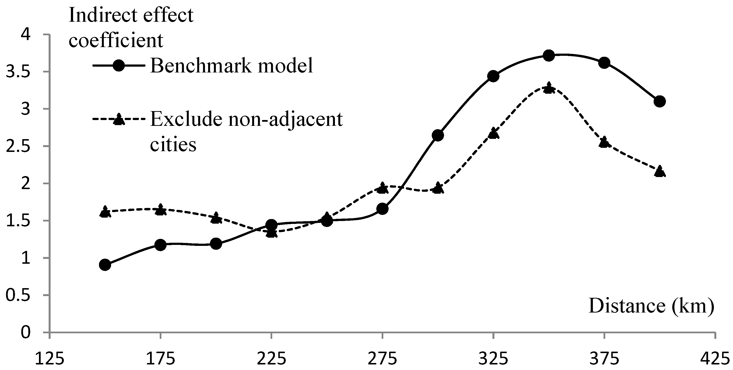
4.2.1. Change the City Sample

Since the minimum distance between some cities is still greater than 150 km, the urban agglomeration was recalculated after excluding the above 20 cities.

Table 4. Results of excluding non-adjacent cities.

IC	(1)	(2)	(3)	(4)	(5)	(6)
Distance	150 km	175 km	200 km	225 km	250 km	275 km
Direct effect	−0.2166 (−0.995)	−0.3543 (−1.3961)	−0.1146 (−0.4027)	−0.0704 (−0.2381)	−0.2398 (−0.7578)	−0.3454 (−1.0263)
Indirect effect	1.6235 *** (5.7552)	1.5411 *** (4.6875)	1.5414 *** (3.648)	1.3531 *** (2.988)	1.541 *** (2.8037)	1.9436 *** (3.1436)
Total effect	1.4069 *** (5.0735)	1.2968 *** (4.2107)	1.4267 *** (3.8941)	1.2827 *** (3.0881)	1.3012 *** (2.6228)	1.5983 *** (2.7686)
IC	(7)	(8)	(9)	(10)	(11)
Distance	300 km	325 km	350 km	375 km	400 km
Direct effect	−0.3105 (−0.8114)	−0.6687 * (−1.7479)	−1.1319 ** (−2.4366)	−0.5869 (−1.1348)	−0.2486 (−0.5067)
Indirect effect	1.9446 *** (2.7824)	2.6792 *** (3.6255)	3.2875 *** (3.8121)	2.5587 ** (2.5206)	2.1666 ** (2.0818)
Total effect	1.6342 *** (2.6562)	2.0104 *** (2.9201)	2.1556 *** (2.8375)	1.9718 ** (2.1722)	1.918 ** (2.0245)

Note: The number of cities is 258. ***, **, and * represent significance of 1%, 5%, and 10%, respectively.

presents the regression results. The direct coefficients are all negative, and the significance decreased. The reason may be that the excluded cities are located in peripheral areas within a relatively low degree of agglomeration. The indirect effects show an inverted U-shaped relationship with the expansion of distance in Figure 1, and all of them are positive and significant, which is consistent with the previous results, showing the robustness of the conclusion.

4.2.2. Change the Explanatory Variables of Registered Population

There are two effects of using the registered population data to calculate the urban agglomeration. One is to underestimate the size of large cities and overestimate the size of small- and medium-sized cities. Second, the deviation of agglomeration degree caused by city scale will be reduced with the expansion of agglomeration scope.

Table 5. Results of using registered population data.

IC	(1)	(2)	(3)	(4)	(5)	(6)
Distance	150 km	175 km	200 km	225 km	250 km	275 km
Direct effect	0.0655 (0.5717)	−0.1366 (−1.1091)	−0.2123 * (−1.6647)	−0.3115 ** (−2.1696)	−0.2866 * (−1.9269)	−0.4272 *** (−2.7533)
Indirect effect	0.8249 *** (4.5902)	1.1019 *** (5.4473)	1.3274 *** (5.8056)	1.6114 *** (6.0174)	1.6414 *** (5.5811)	1.9489 *** (5.8244)
Total effect	0.8904 *** (5.7992)	0.9653 *** (5.575)	1.1151 *** (5.3346)	1.2999 *** (5.2612)	1.3548 *** (5.0461)	1.5217 *** (5.2055)
IC	(7)	(8)	(9)	(10)	(11)
Distance	300 km	325 km	350 km	375 km	400 km
Direct effect	−0.5441 * (−1.7653)	−0.7236 ** (−2.4161)	−0.8208 ** (−2.5111)	−1.0518 *** (−2.9032)	−1.0825 *** (−2.7252)
Indirect effect	1.6042 *** (3.9137)	1.8779 *** (4.2519)	1.9691 *** (3.9649)	2.2838 *** (4.0969)	2.2989 *** (4.1253)
Total effect	1.0601 *** (3.6492)	1.1544 *** (3.473)	1.1483 *** (2.9475)	1.232 *** (3.0994)	1.2164 *** (3.0782)

Note: ***, **, and * represent significance of 1%, 5%, and 10%, respectively.

gives the robustness test results of using registered population data. The deviation makes the direct effect coefficient start to turn negative at 175 km. The permanent population of most small- and medium-sized cities is much lower than the registered population, and the distance between these cities is small. The overestimation of the urban agglomeration degree puts the city in the process of transition from agglomeration economy to agglomeration diseconomy at a small distance. This also means that adjusting the spatial distribution of the population helps to mitigate the negative effects of agglomeration diseconomies. The indirect effect coefficients are all positive and significant, which further confirms the significant spillover effect of urban agglomeration on the development of surrounding areas. In Figure 2, the coefficients are roughly equal to the results of the permanent population within 275 km. However, beyond 300 km, the coefficients are significantly lower than the spillover effects calculated of the registered population. Although the expansion of distance reduces the bias of city size, the degree of urban agglomeration in large cities may still be underestimated, resulting in the failure of large cities to reach an effective size to exert agglomeration spillovers. In addition, the indirect effect coefficient exhibits a fluctuating upward trend and does not show an obvious inflection point. Since the permanent population data can better reflect the current agglomeration status of cities, its use for analysis will lead to more accurate conclusions.

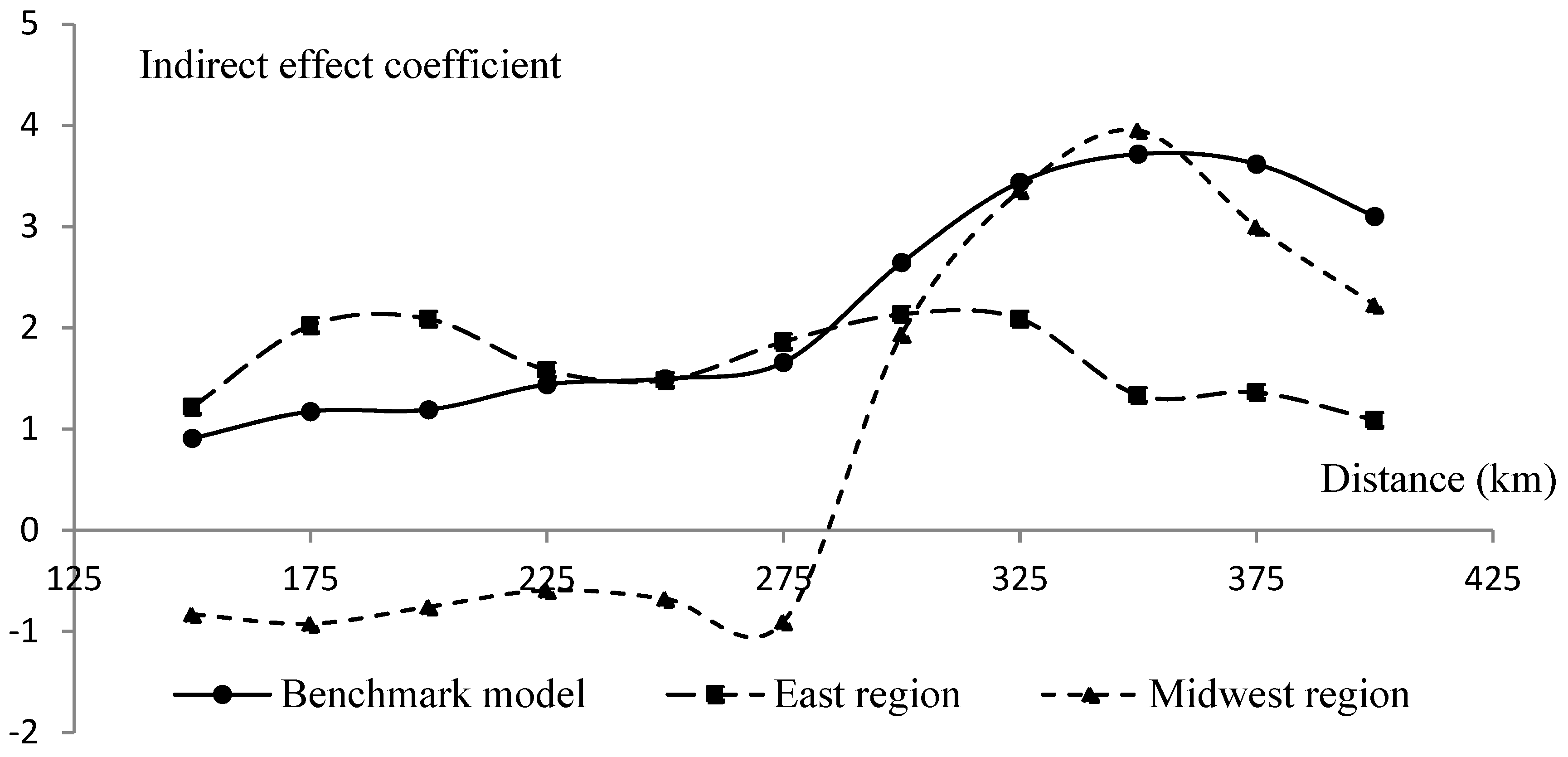
4.3. Heterogeneity Analysis

China’s spatial economic development exhibits significant coastal-inland differences, and the growth and spillover effects of urban agglomeration in different regions are the basic prerequisites for implementing differentiated policies. From the results in

Table 6. Results of east region.

IC	(1)	(2)	(3)	(4)	(5)	(6)
Distance	150 km	175 km	200 km	225 km	250 km	275 km
Direct effect	0.2116 (1.1039)	0.0178 (0.0868)	0.3754* (1.7555)	0.2454 (1.0555)	0.3768 (1.6231)	0.3314 (1.3048)
Indirect effect	1.2163 *** (3.6067)	2.0219 *** (5.0902)	2.0863 *** (4.4102)	1.5811 *** (3.6534)	1.4797 *** (3.2918)	1.8606 *** (3.1876)
Total effect	1.4278 *** (3.5717)	2.0397 *** (4.8055)	2.4617 *** (4.9645)	1.8265 *** (4.0381)	1.8566 *** (4.0168)	2.1919 *** (3.9108)
IC	(7)	(8)	(9)	(10)	(11)
Distance	300 km	325 km	350 km	375 km	400 km
Direct effect	0.033 (0.1086)	0.1278 (0.409)	0.4524 (1.298)	0.5912 (1.6363)	0.6526 * (1.8567)
Indirect effect	2.1329 *** (3.5981)	2.0869 *** (3.3999)	1.3348 * (1.9464)	1.3616 * (1.9149)	1.0866 (1.4703)
Total effect	2.1669 *** (3.9385)	2.2147 *** (3.9463)	1.7872 *** (2.9275)	1.9528 *** (3.1323)	1.7392 ** (2.543)

Note: ***, **, and * represent significance of 1%, 5%, and 10%, respectively.

, the direct effects in the eastern region are all positive, but mostly insignificant. The eastern coastal area itself has a large population, and the continuous inflow of population from the central and western regions has led to a higher degree of urban agglomeration in the eastern region, showing a positive effect on its development. Cities with different functions, geographic locations, and natural conditions may achieve different optimal urban agglomeration conditions. Obviously, cities in the eastern region have higher carrying capacity and greater economies of scale. Therefore, although the urban agglomeration degree in this region is relatively high, it has not crossed the critical point and may be in the process of transition to agglomeration diseconomy.

Figure 3 gives the results of different regions. The indirect effect coefficient roughly exhibits an M-shaped curve and reaches the maximum at 200 and 300 km, respectively. The indirect effect coefficients are positively significant at all distances. As shown in Figure 3, the spillover effect in the eastern region is higher than the benchmark model within 275 km distance, indicating a greater agglomeration growth effect. This is due to several factors, such as higher urban agglomeration degree, closer city spacing, and more core cities. It is also in line with the regular pattern of economic activities and the population is concentrated in geographically advantageous areas. The spillover effect is flat or even declining at a larger scale. The reason may be that an effective industrial division of labor is not established in a broader region, and some cities have competitive effects for factors and resources.

The results of the central and western regions are distinguished by the 275 km in column 6 of

Table 7. Results of midwest region.

IC	(1)	(2)	(3)	(4)	(5)	(6)
Distance	150 km	175 km	200 km	225 km	250 km	275 km
Direct effect	0.596 *** (3.041)	0.7285 *** (3.3859)	1.1224 *** (5.0165)	0.9762 *** (4.3666)	0.9072 *** (3.9389)	1.2059 *** (5.1618)
Indirect effect	−0.8312 ** (−2.3243)	−0.9238 * (−1.9565)	−0.757 (−1.1956)	−0.5943 (−0.7768)	−0.6774 (−0.8033)	−0.9032 (−0.988)
Total effect	−0.2352 (−0.6044)	−0.1953 (−0.3871)	0.3654 (0.5483)	0.382 (0.4733)	0.2297 (−0.2604)	0.3027 (0.3187)
IC	(7)	(8)	(9)	(10)	(11)
Distance	300 km	325 km	350 km	375 km	400 km
Direct effect	−0.485 (−1.0397)	−0.6164 * (−1.6767)	−0.6303 (−1.5724)	0.0179 (0.037)	0.8298 ** (1.9819)
Indirect effect	1.9352 * (1.784)	3.3556 *** (3.4445)	3.9488 *** (3.931)	2.996 ** (2.6041)	2.226 ** (2.013)
Total effect	1.4502 (1.4503)	2.7392 *** (2.7737)	3.3185 *** (3.216)	3.0139 *** (2.6139)	3.0558 *** (2.7167)

Note: ***, **, and * represent significance of 1%, 5%, and 10%, respectively.

. It is consistent with the growth trend performance before 275 km in the benchmark model. Within this distance, the urban agglomeration has a significant promoting effect on its own development, while the indirect coefficients are negative and insignificant. Beyond 300 km, the direct effect turns negative, while the agglomeration spillover effect of large cities begins to affect peripheral cities. The indirect effect also shows an inverted U-shaped curve relationship in this distance interval. Cities with a small size and low urban agglomeration degree in the central and western regions show weak economies of scale. Most cities are in the stage with the continuous expansion of agglomeration advantages. Thus, urban agglomeration can generate growth advantages for local development on a small scale. In a larger space, it has a negative impact because it is difficult to support economic activities that exceed its own carrying capacity. In addition, the large urban spacing and few central cities weaken the radiation effect of the core cities on peripheral cities in the central and western regions to a certain extent. Therefore, there are insufficient spatial connections on a smaller scale to bring out the agglomeration spillover from the core city. In addition, most small and medium-sized cities show a fierce competition effect due to economic development goals. Only at larger distances can core cities form spatial connections with most small- and medium-sized cities and have significant spillover effects on backward areas with lower agglomeration levels.

4.4. Further Analysis

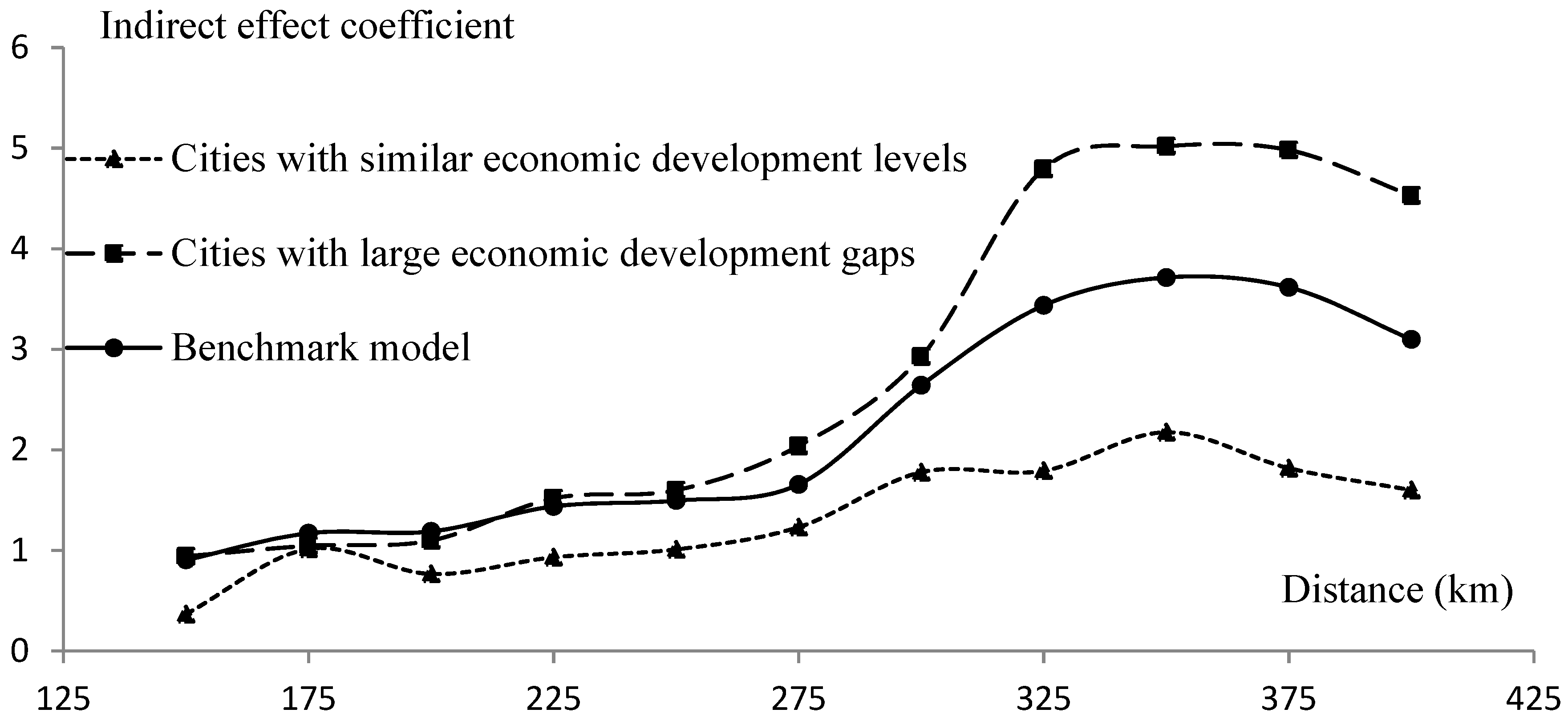
4.4.1. Economic Distance Moderation Effect

Economic distance reflects the disparity in economic development levels between cities, and this subsection examines the moderating effect of regional development differences on agglomeration effects. The economic distance matrix is constructed by the distance and the average GDP per capita from 2010–2019. Matrix 4 emphasizes the interaction between cities with large economic development gap. Matrix 5 emphasizes the interaction between cities with similar economic development levels.

$$W_{e1}=\frac{\left|\overline{{gdp}_i}-\overline{{gdp}_j}\right|}{d_{ij}},{d<d}_d,i\ne j$$

(4)

$$W_{e2}=\frac{1}{\left|\overline{{gdp}_i}-\overline{{gdp}_j}\right|}\cdot \frac{1}{d_{ij}},{d<d}_d·i\ne j$$

(5)

The results of the economic distance matrix in

Table 8. Results of using economic distance matrix 4.

IC	(1)	(2)	(3)	(4)	(5)	(6)
Distance	150 km	175 km	200 km	225 km	250 km	275 km
Direct effect	0.437 *** (2.8847)	0.1795 (1.04)	0.3953 ** (2.2826)	0.1549 (0.8116)	0.1148 (0.5904)	0.101 (0.5004)
Indirect effect	0.943 *** (4.1883)	1.0473 *** (4.0148)	1.0993 *** (3.6665)	1.5189 *** (4.6073)	1.6004 *** (4.4911)	2.0405 *** (4.979)
Total effect	1.3801 *** (5.8025)	1.2268 *** (4.8942)	1.4946 *** (4.8796)	1.6739 *** (4.9351)	1.7152 *** (4.6705)	2.1416 *** (5.343)
IC	(7)	(8)	(9)	(10)	(11)
Distance	300 km	325 km	350 km	375 km	400 km
Direct effect	−1.0339 *** (−2.8686)	−1.64 *** (−4.899)	−1.6841 *** (−4.1372)	−1.7011 *** (−3.6377)	−1.274 *** (−2.6286)
Indirect effect	2.9279 *** (5.4703)	4.7943 *** (8.2124)	5.0194 *** (7.2699)	4.9813 *** (6.8728)	4.5296 *** (5.7811)
Total effect	1.8939 *** (3.7943)	3.1543 *** (5.6988)	3.3354 *** (5.3657)	3.2802 *** (5.3193)	3.2556 *** (4.7731)

Note: ***, ** represent significance of 1%, 5%, respectively.

and

Table 9. Results of using economic distance matrix 5.

IC	(1)	(2)	(3)	(4)	(5)	(6)
Distance	150 km	175 km	200 km	225 km	250 km	275 km
Direct effect	0.5186 *** (3.8638)	0.1518 (1.0105)	0.3811 ** (2.499)	0.2255 (1.4059)	0.2543 (1.5403)	0.0944 (0.5472)
Indirect effect	0.3684 ** (1.9726)	1.0167 *** (4.58)	0.7668 *** (3.0418)	0.9333 *** (3.5676)	1.0113 *** (3.8174)	1.2331 *** (4.2872)
Total effect	0.8871 *** (4.6172)	1.1684 *** (5.509)	1.1479 *** (4.6361)	1.1588 *** (4.5221)	1.2657 *** (4.9603)	1.3276 *** (5.1997)
IC	(7)	(8)	(9)	(10)	(11)
Distance	300 km	325 km	350 km	375 km	400 km
Direct effect	−0.6434 ** (−2.3541)	−0.7227 ** (−2.5136)	−1.0606 *** (−3.1373)	−0.7283 * (−1.8798)	−0.6545 (−1.5718)
Indirect effect	1.7787 *** (5.0645)	1.7933 *** (4.651)	2.1768 *** (4.9028)	1.8192 *** (3.6779)	1.6013 *** (3.0538)
Total effect	1.1353 *** (4.022)	1.0706 *** (3.6979)	1.1162 *** (3.6571)	1.0909 *** (3.4659)	0.9468 *** (2.8104)

Note: ***, **, and * represent significance of 1%, 5%, and 10%, respectively.

indicate that the indirect effect coefficients of urban agglomeration in both matrix forms are positive and significant. From Figure 4, it can be seen that both matrix results demonstrate a clear inverted U-shaped curve. In addition, the curve considering cities with large economic development gap are higher than the curve of cities with similar economic development levels, indicating that the spillover effect of urban agglomeration is stronger among cities with large development differences. This result suggests that cities with different levels of economic development are more likely to form complementary relationships. Large cities optimize their own development space with small- and medium-sized cities, while backward cities take advantage of the agglomeration effects of large cities to fully realize their development potential, thereby achieving a win-win development situation. The indirect effect coefficient of matrix 5 is smaller than the result of benchmark model at each distance. It can be seen that when the level of economic development is similar between cities, the similarity of demand for resources and factors makes it easier for the two places to form a competitive relationship and offset the spillover effect of urban agglomeration. Especially in small- and medium-sized cities, economic performance as the main mechanism for assessing the promotion of government officials reinforces the intensity of competition for resources and factors.

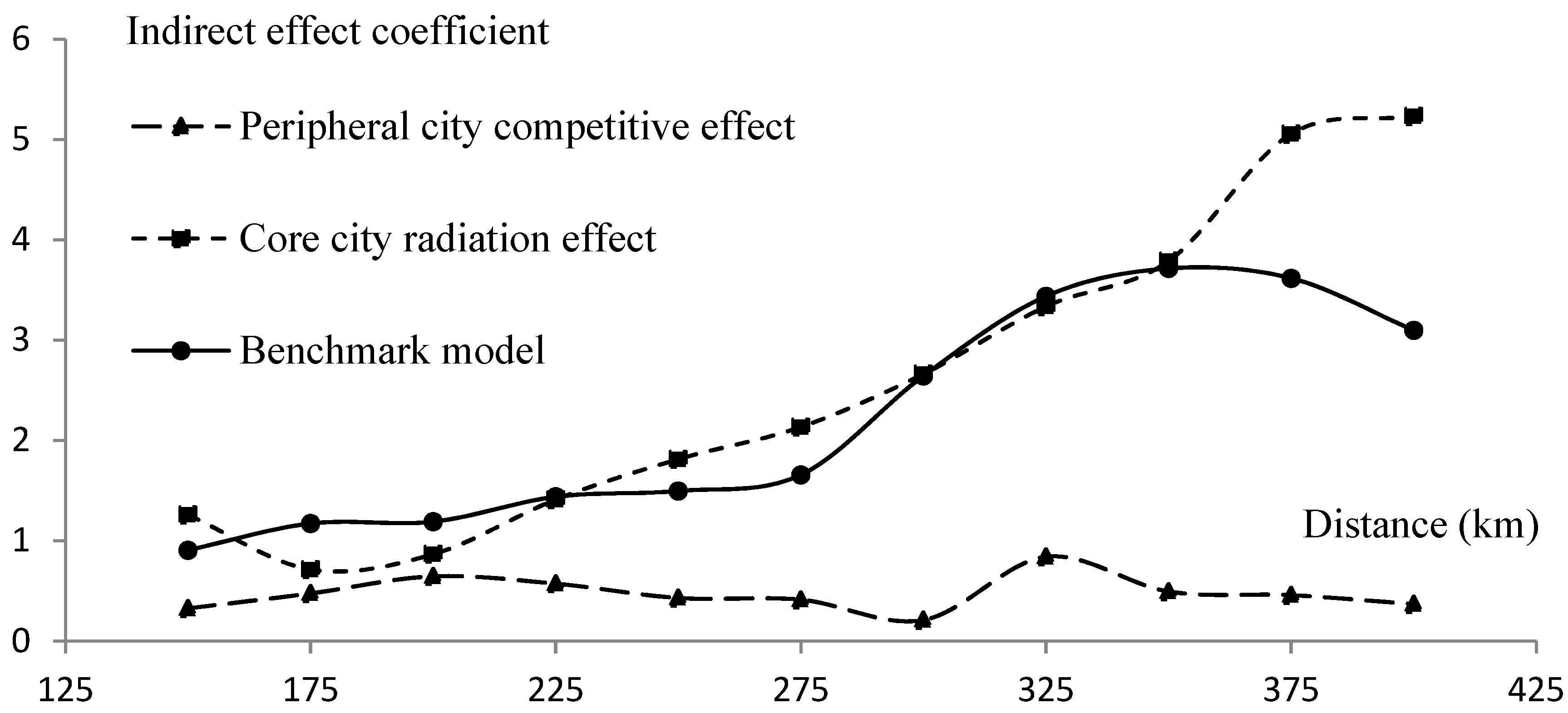
4.4.2. Core City Radiation Effect and Peripheral City Competitive Effect

Regional development is accompanied by the evolution of the core-peripheral structure, and some cities are also defined as core cities in the process of calculating urban agglomeration degree. To analyze the radiation effect of the core city, the competition effect between peripheral cities, and the direction of spatial interactions, the distance matrix with city categories is set up for investigation.

$$W_{ii}=\frac{1}{d_{ij}},\hspace{1em}{d<d}_d,\hspace{1em}i\ne j,$$

(6)

City i and j are the core city and the peripheral city, respectively.

$$W_{ij}=\frac{1}{d_{ij}},\hspace{1em}{d<d}_d,\hspace{1em}i\ne j,$$

(7)

City i and j are both central cities or peripheral cities, which is opposite to matrix 6.

In Figure 5, the interaction between core cities and peripheral cities shows a steady growth trend with distance expansion after 175 km and the coefficients are all positive and significant in

Table 10. Results of core city radiation effect.

IC	(1)	(2)	(3)	(4)	(5)	(6)
Distance	150 km	175 km	200 km	225 km	250 km	275 km
Direct effect	1.0417 *** (7.8868)	1.0157 *** (7.5224)	0.9956 *** (7.1358)	0.6435 *** (4.3539)	0.5909 *** (3.9155)	0.4272 *** (2.6652)
Indirect effect	1.2583 *** (4.8917)	0.7138 *** (2.844)	0.8658 *** (3.2035)	1.4106 *** (5.0154)	1.8136 *** (6.4525)	2.1341 *** (7.0944)
Total effect	2.3 *** (8.2748)	1.7294 *** (6.6014)	1.8615 *** (6.3801)	2.0542 *** (7.0143)	2.4045 *** (8.6499)	2.5613 *** (8.3447)
IC	(7)	(8)	(9)	(10)	(11)
Distance	300 km	325 km	350 km	375 km	400 km
Direct effect	0.3964 ** (2.02)	0.0271 (0.1262)	−0.2840 (−0.9878)	−0.918 *** (−2.7247)	−0.8356 ** (−2.5249)
Indirect effect	2.6625 *** (7.5039)	3.3359 *** (8.2863)	3.7887 *** (7.7771)	5.0563 *** (8.9536)	5.2311 *** (8.5871)
Total effect	3.059 *** (9.0635)	3.363 *** (9.1787)	3.5038 *** (8.8737)	4.1382 *** (8.9766)	4.3956 *** (8.6654)

Note: ***, ** represent significance of 1%, 5%, respectively.

. That means that the radiation effect of the core city on the peripheral cities dominates the agglomeration spillover effect, while the indirect effects of interaction between similar cities in

Table 11. Results of peripheral city competitive effect.

IC	(1)	(2)	(3)	(4)	(5)	(6)
Distance	150 km	175 km	200 km	225 km	250 km	275 km
Direct effect	0.6388 *** (4.7912)	0.5207 *** (3.1095)	0.7165 *** (4.2706)	0.6663 *** (3.7548)	0.7149 *** (3.8973)	0.7553 *** (4.0112)
Indirect effect	0.3255 (1.3594)	0.4749 * (1.8243)	0.645 ** (2.1902)	0.5725 * (1.8226)	0.4297 (1.2777)	0.4125 (1.1194)
Total effect	0.9643 *** (3.8691)	0.9956 *** (3.9712)	1.3615 *** (4.686)	1.2388 *** (3.9479)	1.1446 *** (3.5344)	1.1678 *** (3.4925)
IC	(7)	(8)	(9)	(10)	(11)
Distance	300 km	325 km	350 km	375 km	400 km
Direct effect	1.2332 *** (5.0094)	0.9662 *** (4.0288)	0.9548 *** (3.4923)	0.7809 ** (2.537)	0.9395 *** (2.9124)
Indirect effect	0.2102 (0.5174)	0.8404 * (1.9214)	0.4936 (0.9777)	0.4575 (0.7852)	0.3691 (0.6295)
Total effect	1.4434 *** (3.8508)	1.8066 *** (4.4399)	1.4484 *** (3.2298)	1.2385 ** (2.5042)	1.3086 *** (2.6135)

Note: ***, **, and * represent significance of 1%, 5%, and 10%, respectively.

are positive but hardly significant. Furthermore, they are all smaller than the benchmark model at the corresponding distances. The results demonstrate that there is a strong competitive effect among similar cities, especially among peripheral cities. The findings are consistent with the moderating effect of economic distance above. To sum up, in terms of the direction of the spillover effect of agglomeration, it is mainly manifested between high-ranking cities and low-ranking cities, and there is an obvious competition effect between similar cities.

4.4.3. Integration Effect

Integration is an important driving force for urban economic development. In the context of the transformation of administrative economies to urban cluster economies, the role of urban agglomeration on regional growth is significantly different under the influence of inter-provincial boundaries. The existence of administrative barriers makes the local government aim to maximize the benefits and minimize the cost within the administrative boundaries, resulting in the fragmentation of the regional market and hinder integrated development. The existence of inter-provincial administrative boundaries leads to market segmentation to a certain extent and also hinders the spillover effect from core cities to regions outside the province. In order to investigate the impact of provincial administrative boundaries on agglomeration spillovers, the urban agglomeration degree is recalculated based on the population of the city in the province where the city is located, that is, only the population of cities in the same province as the target city is considered. Cities outside the province are not counted even if they are within a given distance. The spatial matrix also only considers the spatial interaction of two cities in the same province at a certain distance. Since the municipality is a provincial administrative unit, it is still handled in accordance with the benchmark model.

In

Table 12. Results of integration effect.

IC	(1)	(2)	(3)	(4)	(5)	(6)
Distance	150 km	175 km	200 km	225 km	250 km	275 km
Direct effect	0.7683 *** (5.4441)	0.3698 ** (2.5116)	0.6797 *** (4.3471)	0.4499 *** (2.6278)	0.6786 *** (3.7669)	0.5167 *** (2.8168)
Indirect effect	0.3626 * (1.7284)	0.9498 *** (4.0395)	1.0736 *** (3.9107)	1.2828 *** (4.1567)	1.1621 *** (3.5427)	1.5357 *** (4.2322)
Total effect	1.1309 *** (5.1473)	1.3196 *** (5.6949)	1.7533 *** (6.3784)	1.7327 *** (5.5057)	1.8407 *** (5.6041)	2.0524 *** (6.1021)
IC	(7)	(8)	(9)	(10)	(11)
Distance	300 km	325 km	350 km	375 km	400 km
Direct effect	0.6027 *** (2.9557)	0.6483 *** (3.1596)	0.6212 *** (2.9206)	0.7212 *** (3.2268)	0.8282 *** (3.5358)
Indirect effect	1.4844 *** (4.2495)	1.6412 *** (4.348)	1.7262 *** (4.365)	1.721 *** (4.122)	1.716 *** (3.8212)
Total effect	2.087 *** (5.6091)	2.2895 *** (5.8188)	2.3475 *** (5.8131)	2.4421 *** (5.9939)	2.5442 *** (5.5224)

Note: ***, **, and * represent significance of 1%, 5%, and 10%, respectively.

, the direct effect coefficients are all significantly positive and pass the significance test at the level of 1%. The indirect effect coefficients are all significantly positive, but as shown in Figure 6, after considering the influence of the administrative boundary, the indirect effect coefficients are all smaller than the results without market segmentation under the corresponding distance, reflecting that an integrated development strategy plays a crucial role in promoting the spatial externalities of urban agglomeration. As cities become increasingly connected, the smaller the administrative barriers between regions, the stronger the economic externalities of the region as a whole. The difference between the two results is relatively small within 275 km and shows a very obvious gap between 300 km and 400 km. The reason may be that the core city is usually located in the hinterland of the province and cannot effectively interact with the cities in the border area at a relatively small distance, so there is no significant difference from the results of the benchmark model. However, at a relatively large distance, considering the results of administrative boundaries, only the agglomeration spillover effect of core cities on cities in the same province is estimated, ignoring the impact of border areas on other provincial cities, and this impact on small cities in border areas is very significant, and thus far from the benchmark model results.

4.4.4. Industrial Diversification and Industrial Specialization Effect

To further analyze the impact of industrial development on urban economies from the perspective of agglomeration externalities, the specialization and diversification indicators are added to the benchmark model. The location quotient is selected as the estimator of industrial specialization.

$$L_{ij}=\frac{{e_{ij}/e}_i}{e_j/e},spec=\mathit{max}(L_{ij})$$

(8)

$L_{ij}$ represents the location quotient, $e_{ij}$ represents the number of employees in the j-th industry of the i-th city, $e_i$ represents the total number of employees in city i, $e_j$ represents the employees of industry j across the entire region.

The industrial specialization of the city is set as the maximum industrial location quotient. The Herfindahl–Hirschman Index is used to measure industrial diversification.

$$diver={1/{\displaystyle \sum _j\left(e_{ij}/e_i\right)}}^2$$

(9)

From the results in

Table 13. Results of direct effects from industrial perspective.

Direct effect	(1)	(2)	(3)	(4)	(5)	(6)
Distance	150 km	175 km	200 km	225 km	250 km	275 km
IC	0.6657 *** (4.2152)	0.2337 (1.3177)	0.4417 ** (2.5556)	0.2128 (1.1877)	0.1892 (1.0065)	0.181 (0.941)
Diver	−0.0089 *** (−3.4919)	−0.0099 *** (−4.1323)	0.0108 *** (−4.6299)	−0.0102 *** (−4.1819)	−0.0102 *** (−4.3302)	−0.0103 *** (−4.4918)
Spec	0.0071 ** (2.1961)	0.005 (1.5652)	0.0053 * (1.6819)	0.0081 *** (2.6524)	0.0084 *** (2.8791)	0.0095 *** (3.1337)
Direct effect	(7)	(8)	(9)	(10)	(11)
Distance	300 km	325 km	350 km	375 km	400 km
IC	−0.8365 ** (−2.5186)	−1.1362 *** (−3.2873)	−1.5284 *** (−3.8041)	−1.4348 *** (−3.2539)	−1.18441 ** (−2.5783)
Diver	−0.0098 *** (−4.101)	−0.0093 *** (−4.0318)	−0.0094 *** (−3.9078)	−0.0099 *** (−4.0363)	−0.0101 *** (−4.3721)
Spec	0.0083 *** (2.8489)	0.008 *** (2.6577)	0.0083 *** (2.6588)	0.0075 ** (2.4143)	0.0075 ** (2.4139)

Note: ***, **, and * represent significance of 1%, 5%, and 10%, respectively.

and

Table 14. Results of indirect effects from industrial perspective.

Indirect effect	(1)	(2)	(3)	(4)	(5)	(6)
Distance	150 km	175 km	200 km	225 km	250 km	275 km
IC	0.977 *** (3.7616)	1.1834 *** (3.9536)	1.2799 *** (3.7461)	1.5683 *** (3.9444)	1.554 *** (3.4994)	1.6934 *** (3.4253)
Diver	−0.001 (−0.181)	0.0048 (0.7852)	0.0072 (1.039)	0.0015 (0.1777)	−0.0034 (−0.3499)	−0.0035 (−0.3191)
Spec	−0.0196 *** (−3.0219)	−0.019 ** (−2.2895)	−0.0252 *** (−2.8396)	−0.0267 ** (−2.297)	−0.024 * (−1.7079)	−0.279 * (−1.6776)
Indirect effect	(7)	(8)	(9)	(10)	(11)
Distance	300 km	325 km	350 km	375 km	400 km
IC	2.4912 *** (3.9756)	3.3085 *** (4.505)	3.7208 *** (4.5379)	3.7229 *** (4.0523)	3.2893 *** (3.3534)
Diver	0.0188 (1.4182)	0.0206 (1.4506)	0.0215 (1.2959)	0.0126 (0.7031)	0.0111 (0.5451)
Spec	−0.0394 ** (−2.1192)	−0.0436 ** (−2.0149)	−0.0404 ** (−1.661)	−0.0569 ** (−2.1418)	−0.0628 ** (−2.0875)

Note: ***, **, and * represent significance of 1%, 5%, and 10%, respectively.

, it is clear that increased industrial specialization promotes urban economic growth but hurts the development of the surrounding areas. Specialized production is more likely to produce scale effects, reduce production costs, and improve technology levels. Since the specialization index is relative, an increase in the local specialization may lead to a decrease in the peripheral specialization index, thus generating a negative spillover effect.

The diversification of industrial clusters is not conducive to the economic development of cities themselves. The industrial base of small- and medium-sized cities is not sufficient to support the blind pursuit of a “big and comprehensive” industrial development strategy. The coefficients of indirect effects of diversification are not significant. Diversification usually promotes urban growth through the complementarity and knowledge spillover generated by the interaction of different industries. However, at the present stage, most cities have not formed effective industrial linkages, the division of labor is not well coordinated, and the comparative advantages of each city have not been fully exploited.

4.4.5. Urban Network Externalities Perspective

In order to test whether urban network externalities exist and also to examine the differences in their effects on economic growth from this perspective, the urban agglomeration IC is recalculated using railroad travel time instead of geographic distance. That is, IR is the time distance between two cities instead of the geographic straight-line distance. The urban network weight matrix is constructed using railway travel time and frequency data to reflect the strength of interaction between cities.

$$W_{ij}=\left\{\begin{array}{c}0,t_{ij}>t_t\\ \mathit{freq}/t_{ij},t_{ij}<t_t\end{array}\right.$$

(10)

$t_{ij}$ is the time distance between city i and city j, $t_t$ represents the time threshold, freq is the train frequency between the two cities. To further analyze the differences in the results at different spatial scales and the robustness of the conclusions, the results at different temporal distances are investigated.

In terms of the direct effect, the urban agglomeration coefficients in

Table 15. Results of urban network externalities perspective.

IC	(1)	(2)	(3)	(4)	(5)	(6)
Time	1 h	1.5 h	2 h	2.5 h	3 h	3.5 h
Direct effect	0.7618 *** (6.6682)	0.3783 *** (3.2453)	0.5787 *** (4.7975)	0.6063 *** (4.8457)	0.5334 *** (4.2618)	−0.0662 (−0.4087)
Indirect effect	0.2816 * (1.7273)	1.2233 *** (6.3745)	1.3026 *** (6.4979)	1.2533 *** (5.4402)	1.3514 *** (5.127)	2.2085 *** (7.8122)
Total effect	1.0434 *** (5.2424)	1.6026 *** (7.2758)	1.8812 *** (8.7153)	1.8596 *** (7.6742)	1.8848 *** (7.1688)	2.1423 *** (7.9165)
Controls	Yes	Yes	Yes	Yes	Yes	Yes
Individual effect	Yes	Yes	Yes	Yes	Yes	Yes
Time effect	Yes	Yes	Yes	Yes	Yes	Yes
Wald spatial lag	123.35 ***	165.87 ***	166.36 ***	163.37 ***	148.54 ***	162.1 ***
LR spatial lag	50.61 ***	101.09 ***	93.56 ***	94.77 ***	93.88 ***	128.82 ***
Wald spatial error	190.69 ***	276 ***	316.87 ***	323.08 ***	315.8 ***	320.55 ***
LR spatial error	84 ***	193.29 ***	204.18 ***	220.75 ***	235.05 ***	301.15 ***
IC	(7)	(8)	(9)	(10)	(11)
Time	4 h	4.5 h	5 h	5.5 h	6 h
Direct effect	−0.177 (−1.0496)	−0.1208 (−0.7209)	−0.5385 ** (−2.5691)	−0.7029 *** (−3.7421)	−0.7813 *** (−3.7131)
Indirect effect	2.4911 *** (8.4797)	2.5618 *** (8.2113)	3.0984 *** (8.657)	3.2865 *** (9.8659)	3.407 *** (9.477)
Total effect	2.3141 *** (8.101)	2.441 *** (8.2476)	2.5599 *** (8.1072)	2.5836 *** (8.3067)	2.6257 *** (8.1331)
Controls	Yes	Yes	Yes	Yes	Yes
Individual effect	Yes	Yes	Yes	Yes	Yes
Time effect	Yes	Yes	Yes	Yes	Yes
Wald spatial lag	174.8 ***	172.56 ***	173.37 ***	193.76 ***	180.5 ***
LR spatial lag	136.4 ***	129.06 ***	141.47 ***	160.9 ***	167.17 ***
Wald spatial error	326.39 ***	329.79 ***	312.12 ***	323.92 ***	303.9 ***
LR spatial error	330.46 ***	303.11 ***	319.52 ***	337.05 ***	338.65 ***

Note: ***, **, and * represent significance of 1%, 5%, and 10%, respectively.

are positive and significant up to 3 h and shift to negative at 3.5 h, showing the same transformation process from agglomeration economic effect to agglomeration diseconomies. This is consistent with the empirical results obtained using geographic distance. The coefficients are all significant at the 1% significance level up to 3 h, while the results calculated using geographical distance are less significant. It can be seen the improvement of city accessibility largely reinforces the positive impact of the agglomeration effect.

The indirect effect coefficients are positive and significant at all time thresholds, confirming the existence of network externalities and their positive impact on the growth of neighboring cities. The coefficients do not show an obvious decreasing trend with the expansion of the considered spatial scale but keep expanding with the expansion of the temporal distance, which is different from the externality that shows an inverted U-shaped curve with geographic distance. Along with the development of transportation and communication technologies, inter-city connectivity and economic ties have increased, and the establishment of city network systems has enabled agglomeration economies to break through the limits of geographical distance and exhibit stronger spatial spillover effects on a larger spatial scale.

5. Conclusions and Recommendations

5.1. Main Conclusions

Using panel data from 278 cities in China from 2010 to 2019, this paper examines the impact of urban agglomeration on urban development under the distance factor based on the spatial Durbin model. The conclusions are as follows: The distance sensitivity of urban agglomeration to urban economic growth cannot be neglected, and a moderate geospatial scale can help cities overcome scale deficiencies and the problem of overcrowding. Geographical proximity is no longer a prerequisite for agglomeration spillover effects. With the construction of transportation infrastructure networks and the rapid development of communication technologies, non-adjacent cities also interact and share agglomeration advantages. The spillover effect of urban agglomeration shows an inverted U-shaped curve with the expansion of geographic distance, and the integration trend further strengthens the positive spillover effect, especially at a relatively large spatial scale. The spatial spillover effect of urban agglomeration also exhibits regional heterogeneity and spatial scale sensitivity, which indicates that there are certain distance thresholds for the spillover effect. Furthermore, the research finds that the direction of spatial interactions is more manifested between high-ranking and low-ranking cities. Specifically, the spillover effects of agglomeration are prominent between cities with larger gaps in economic development levels, especially the core and peripheral cities. Cities with similar development conditions exhibit a competitive effect, which may offset the positive spillover effect. In other words, core cities play an important leading and radiating role in the regional development process. From the industrial agglomeration perspective, increased specialization is more conducive to local growth. The industrial base of most cities is not sufficient to support diversified development. From the urban network externality perspective, the spillover effect of urban agglomeration does not exhibit a diminished tendency with the expansion of spatial scale but shows a more significant effect along with the strengthening of urban linkages. This demonstrates that network externalities will play an increasingly important role in urban economic development.

5.2. Policy Recommendations

Promote the trend of concentration of population and production factors to further exploit the advantages of agglomeration. Rationalize the spatial distribution of population to alleviate the negative effects and agglomeration costs arising from over-agglomeration.

Pay attention to the regulation of local factors on the role of agglomeration, refine regional policy scales, and implement differentiated development strategies. For the western region, it should be alert to the potential risks brought by excessive fragmentation, avoid the agglomeration shadow in neighboring small- and medium-sized cities due to fierce competition, and cultivate a number of regional central cities by enhancing density and shortening distance.

Promote the construction of large cities in a way that is conducive to the development of small- and medium-sized cities. Strengthen the agglomeration intensity of central cities to effectively play its radiation and driving role for the peripheral and backward areas.

Encourage integrated development, break the fetters of inter-provincial administrative boundaries, reduce market segmentation, and realize the maximization of agglomeration spillover effect in the surrounding areas.

Lay out the urban industrial system in a scientific and reasonable way. Develop and grow leading industries, gradually build and optimize the urban industrial division of labor and collaboration system, and enhance the complementary functions of urban industries.

Balance agglomeration externality and network externality and expand and extend the channels and ways for cities to connect. Strengthen the construction of transportation infrastructure and reduce the spatial and temporal distance between cities to better utilize the city borrowed size and network externality.

References

1. Brezzi, M.; Veneri, P. Assessing Polycentric Urban Systems in the OECD: Country, Regional and Metropolitan Perspectives. Eur. Plan. Stud. 2014, 23, 1128–1145. [Google Scholar] [CrossRef]
2. Gardiner, B.; Martin, R. Does spatial agglomeration increase national growth? Some evidence from Europe. J. Econ. Geogr. 2011, 11, 979–1006. [Google Scholar] [CrossRef] [Green Version]
3. Wetwitoo, J.; Kato, H. High-speed rail and regional economic productivity through agglomeration and network externality: A case study of inter-regional transportation in Japan. Case Stud. Transp. Policy 2017, 5, 549–559. [Google Scholar] [CrossRef]
4. Cheng, C.; Zhang, Y.; Chen, D. Influences of urban agglomeration on the quality of economic development: Taking the Yangtze River Economic Xone as an example. Urban Probl. 2020, 4–13. [Google Scholar]
5. Ding, R.; Xu, B.; Zhang, H. Can Urban Agglomeration Drive Regional Economic Growth? Empirical Analysis Based on Seven State-level Urban Agglomerations. Econ. Geogr. 2021, 41, 37–45. [Google Scholar]
6. Tang, C.; Guan, M.; Dou, J. Understanding the impact of High Speed Railway on urban innovation performance from the perspective of agglomeration externalities and network externalities. Technol. Soc. 2021, 67, 101760. [Google Scholar] [CrossRef]
7. Yuan, Q. Do Urban Clusters Promote the Development of Cities? J. World Econ. 2016, 39, 99–123. [Google Scholar]
8. Han, J.; Gao, M.; Sun, Y. Measurement of City Clusters’ Economic Growth Effects and Analysis of the Influencing Factors. Chin. J. Urban Environ. Stud. 2020, 8, 2050006. [Google Scholar] [CrossRef]
9. Yin, J.; Yang, Z.; Guo, J. Externalities of Urban Agglomerations: An Empirical Study of the Chinese Case. Sustainability 2022, 14, 11895. [Google Scholar] [CrossRef]
10. Yao, C.; Song, D.; Fan, X. Does the small size of cities restrict economic growth? a re-examination from the perspective of two kinds of ‘borrowed-size’. China Popul. Resour. Environ. 2020, 30, 62–71. [Google Scholar]
11. Yan, D.; Wang, Y.; Sun, W.; Li, P. A comparative study on the driving factors and spatial spillover effects of economic growth across different regions of China. Geogr. Res. 2021, 40, 3137–3153. [Google Scholar]
12. Yang, T.; Zhu, Y.; Du, J. Is there a borrowed size in China’s urban agglomerations? Prog. Geogr. 2022, 41, 1156–1167. [Google Scholar] [CrossRef]
13. Burger, M.J.; Meijers, E. Agglomerations and the Rise of Urban Network Externalities. Pap. Reg. Sci. 2016, 95, 5–15. [Google Scholar] [CrossRef]
14. Shi, S. Investigating China’s Mid-Yangtze River economic growth region using a spatial network growth model. Urban Stud. 2020, 14, 2973–2993. [Google Scholar] [CrossRef]
15. Cheng, Y.; Su, X. Review on the urban network externalities. Prog. Geogr. 2021, 40, 713–720. [Google Scholar] [CrossRef]
16. Fujita, M.; Krugman, P.R.; Venables, A. The Spatial Economy: Cities, Regions, and International Trade; MIT Press: Cambridge, MA, USA, 2001. [Google Scholar]
17. Duranton, G.; Puga, D. Microfoundations of Urban Agglomeration Economies. In Handbook of Regional and Urban Economics; Elsevier: Amsterdam, The Netherlands, 2004; Volume 4, pp. 2063–2117. [Google Scholar]
18. Faggio, G.; Silva, O.; Strange, W.C. Heterogeneous Agglomeration. Rev. Econ. Stat. 2017, 99, 80–94. [Google Scholar] [CrossRef] [Green Version]
19. Li, P.; Zhang, X. Agglomeration Externalities of City Cluster: Analysis from Labor Wage Premium. Manag. World 2021, 37, 121–136. [Google Scholar]
20. Rosenthal, S.S.; Strange, W.C. Evidence on the nature and sources of agglomeration economies. In Handbook of Regional and Urban Economics; Elsevier: Amsterdam, The Netherlands, 2006; Volume 4, pp. 2119–2171. [Google Scholar]
21. Glaeser, E.L.; Kallal, H.D.; Scheinkman, J.A.; Shleifer, A. Growth in Cities. J. Polit Econ. 1992, 100, 1126–1152. [Google Scholar] [CrossRef]
22. Henderson, V. The Urbanization Process and Economic Growth: The So-What Question. J. Econ. Growth 2003, 100, 1126–1152. [Google Scholar]
23. Mccann, P.; Acs, Z.J. Globalization: Countries, Cities and Multinationals. Reg. Stud. 2011, 45, 17–32. [Google Scholar] [CrossRef] [Green Version]
24. Parr, J.B. Agglomeration economies: Ambiguities and confusions. Environ. Plan. A 2002, 34, 717–731. [Google Scholar] [CrossRef] [Green Version]
25. Drucker, J.; Feser, E. Regional industrial structure and agglomeration economies: An analysis of productivity in three manufacturing industries. Reg. Sci. Urban Econ. 2012, 42, 1–14. [Google Scholar] [CrossRef]
26. Meeteren, M.; Neal, Z.; Derudder, B. Disentangling agglomeration and network externalities: A conceptual typology. Pap. Reg. Sci. 2016, 95, 55–62. [Google Scholar] [CrossRef] [Green Version]
27. Partridge, M.; Bollman, R.D.; Olfert, M.R.; Alasia, A. Riding the Wave of Urban Growth in the Countryside: Spread, Backwash, or Stagnation? Land Econ. 2007, 83, 128–152. [Google Scholar] [CrossRef]
28. Henry, R. External economies of localization, urbanization and industrial diversity and new firm survival. Pap. Reg. Sci. 2011, 90, 473–502. [Google Scholar]
29. Renard, J.F.B.A. Are there spillover effects between coastal and noncoastal regions in China? China Econ. Rev. 2002, 13, 161–169. [Google Scholar]
30. Dobkins, L.H.; Ioannides, Y.M. Spatial interactions among U.S. cities: 1900–1990. Reg. Sci. Urban Econ. 2001, 31, 701–731. [Google Scholar] [CrossRef] [Green Version]
31. Camagni, R.; Salone, C. Network Urban Structures in Northern Italy: Elements for a Theoretical Framework. Urban Stud. 1993, 30, 1053–1064. [Google Scholar] [CrossRef]
32. Meijers, E.J.; Burger, M.J. Stretching the concept of ‘borrowed size’. Urban Stud. 2017, 54, 269–291. [Google Scholar] [CrossRef]
33. Volgmann, K.; Rusche, K. The Geography of Borrowing Size: Exploring Spatial Distributions for German Urban Regions. Tijdschr. Voor Econ. Soc. Geogr. 2020, 111, 60–79. [Google Scholar] [CrossRef] [Green Version]
34. Vos, D.D.; Lindgren, U.; Ham, M.V.; Meijers, E. Does broadband internet allow cities to ‘borrow size’? Evidence from the Swedish labour market. Reg. Stud. 2020, 54, 1175–1186. [Google Scholar] [CrossRef]
35. Partridge, M.D.; Dan, S.R.; Ali, K.; Olfert, M.R. Do New Economic Geography Agglomeration Shadows Underlie Current Population Dynamics across the Urban Hierarchy? Pap. Reg. Sci. 2009, 88, 445–466. [Google Scholar] [CrossRef]
36. Meijers, E.J.; Burger, M.J.; Hoogerbrugge, M.M. Borrowing size in networks of cities: City size, network connectivity and metropolitan functions in Europe. Pap. Reg. Sci. 2016, 95, 473–502. [Google Scholar] [CrossRef] [Green Version]
37. Camagni, R.; Capello, R.; Caragliu, A. Static vs. dynamic agglomeration economies. Spatial context and structural evolution behind urban growth. Pap. Reg. Sci. 2016, 95, 133–158. [Google Scholar] [CrossRef]
38. Glaeser, E.L.; Ponzetto, G.A.; Zou, Y. Urban Networks: Connecting Markets, People, and Ideas. Pap. Reg. Sci. 2016, 95, 17–59. [Google Scholar] [CrossRef] [Green Version]
39. Capello, R. The City Network Paradigm: Measuring Urban Network Externalities. Urban Stud. 2000, 37, 1925–1945. [Google Scholar] [CrossRef]
40. Huang, Y.; Hong, T.; Ma, T. Urban network externalities, agglomeration economies and urban economic growth. Cities 2020, 107, 102882. [Google Scholar] [CrossRef]
41. Navarro-Azorín, J.M.; Artal-Tur, A. How much does urban location matter for growth? Eur. Plan. Stud. 2017, 25, 298–313. [Google Scholar] [CrossRef]
42. Tabuchi, T.; Thisse, J.F. A new economic geography model of central places. J. Urban Econ. 2011, 69, 240–252. [Google Scholar] [CrossRef]
43. Cuberes, D.; Desmet, K.; Rappaport, J. Urban growth shadows. J. Urban Econ. 2021, 123, 103334. [Google Scholar] [CrossRef]
44. Liu, X.; Wang, A.; Ji, X.; Yang, B. Siphon Effect of Central Cities and Coordinated Development of Regions. China Soft Sci. 2022, 76–86. [Google Scholar]
45. Gong, X.; Zhong, F. The Impact of Borrowing Size on the Economic Development of Small and Medium-Sized Cities in China. Land 2021, 10, 134. [Google Scholar] [CrossRef]
46. Sun, B.; Ding, S. Do Large Cities Contribute to Economic Growth of Small Cities? Evidence from Yangtze River Delta in China. Geogr. Res. 2016, 35, 1615–1625. [Google Scholar]
47. Portnov, B.A.; Erell, E.; Bivand, R.; Nilsen, A. Investigating the Effect of Clustering of the Urban Field on Sustainable Growth of Centrally Located and Peripheral Towns. Int. J. Popul. Geogr. 2000, 6, 133–154. [Google Scholar] [CrossRef]
48. Portnov, B.A.; Erell, E. Clustering of the Urban Field as a Precondition for Sustainable Population Growth in Peripheral Areas: The Case of Israel. Rev. Urban Reg. Dev. Stud. 2007, 10, 123–141. [Google Scholar] [CrossRef]
49. Portnov, B.A.; Schwartz, M. Urban clusters as growth foci. J. Reg. Sci. 2009, 49, 287–310. [Google Scholar] [CrossRef]
50. Li, S.; Zhu, H. Agglomeration Externalities and Skill Upgrading in Local Labor Markets: Evidence from Prefecture-Level Cities of China. Sustainability 2020, 12, 6509. [Google Scholar] [CrossRef]
51. Huang, Y.; Li, L.; Yu, Y. Does urban cluster promote the increase of urban eco-efficiency? Evidence from Chinese cities. J. Clean Prod. 2018, 197, 957–971. [Google Scholar] [CrossRef]
Figure 1. The indirect effect coefficients of benchmark model and robustness test of changing city samples.
Sustainability 14 14512 g001
Figure 2. The indirect effect coefficients of benchmark model and robustness test of registered population.
Sustainability 14 14512 g002
Figure 3. The indirect effect coefficients of different regions.
Sustainability 14 14512 g003
Figure 4. The indirect effect coefficients with economic distance matrix.
Sustainability 14 14512 g004
Figure 5. The indirect effect coefficients with city categories.
Sustainability 14 14512 g005
Figure 6. The indirect effect coefficients of administrative boundary.
Sustainability 14 14512 g006