Abstract
Analyzing the spatial and temporal evolution of ecosystem service value (ESV) and the driving mechanisms of spatial differentiation are fundamental to exploring the sustainable development of regional ecosystems. This article selected a coastal region in southeastern China with rapid economic development as the study object. Based on the five land-use remote sensing data sets from 2000 to 2019, the benefit transfer method was used to evaluate the ESV in the coastal zone of Jiangsu Province, revealing the spatial and temporal evolution characteristics of ESV more accurately. Meanwhile, using the panel data regression model delved into the driving mechanisms of ESV spatial heterogeneity. The results showed the following: (1) There was a marked change in land use types from 2000 to 2019, with significant reductions in cropland and water areas and continued urban land expansion. The overall ESV in the study area exhibited a downward trend (8.41%), with regulation and support services being its core functions. (2) The ESV distribution had a distinct spatial differentiation, with hotspots mainly located near the coastal zone and cold spots in towns and surrounding areas. (3) There were considerable differences in the degree of impact of each influencing factor on different types of ESVs. On the whole, land use intensity had the most significant impact and was the first driver, followed by climate change and socioeconomic factors. The findings indicate that future ecosystem management decision-making should involve the conservation and intensive use of land resources and guide human livelihood and production activities toward ESV preservation and appreciation.
1. Introduction
Ecosystem services refer to all the benefits humans need to survive and thrive in the natural environment through the ecosystem [1]. Natural ecosystems contribute to improved human welfare and progress toward sustainable development by providing food, storing carbon, cleaning the air, protecting biodiversity, regulating local climates, and more [2,3,4,5]. However, increased human activity is damaging the environment and increasing the vulnerability and instability of ecosystems [6]. Over the past half-century, two-thirds of the world’s ecosystem services have deteriorated due to economic development and population growth [7]. Ecosystem service evaluation provides a scientific basis for a deeper understanding of regional ecological changes [8].
With the publication of the Millennium Ecosystem Assessment (MEA, 2005), ecosystem assessment has become the most critical direction for assessing the economic value of nature [9]. By assessing ecosystem service value (ESV) in monetary units, it is possible to quantify the benefits of ecosystems and help decision-makers make optimal decisions about the appropriate allocation of resources [10], as well as having positive implications for the construction of low-carbon eco-cities [11,12]. There are four main approaches to evaluating ESV in monetary units: the stated preference approach, revealed preference approach, cost-based approach, and benefit transfer approach [13]. Among them, the benefit transfer approach takes advantage of the area and value equivalent coefficients of different land use types to compute the ESV and has been widely applied by scholars for its simplicity and ease of implementation [14,15]. However, some scholars point out that the benefit transfer approach is inevitably subjective in determining value equivalence coefficients, and thus has limitations and uncertainties in practical application [15]. Therefore, the value equivalent coefficients should be revised according to the actual ecological environment of the study area when applying the method in different regions. Xie et al. derived the Chinese ESV value equivalence scale after combining field surveys and expert scoring, taking into account the real-life environment in China, which laid the foundation for ESV evaluation in different regions and scales, and has been widely used and validated in the Chinese context [16,17,18,19,20]. Since the ecosystem service equivalence factor directly affects the accuracy of ESV evaluation, it needs to be revised according to the actual situation of the study area when evaluating.
According to the Intergovernmental Science-Policy Platform on Biodiversity and Ecosystem Services (IPBES) global assessment, the world is facing “unprecedented” natural decline and “accelerating” rates of species extinction due to the combined effects of climate change and human activities [21]. Climatic conditions may affect plant reproductive output and the state of meadow communities, alter ecosystem structures and functions, and reduce ecosystem stability, thereby affecting the provision of ecosystem services [22,23]. The impacts of climatic conditions on ecosystems in different regions are positive and negative, with significant spatial heterogeneity [24]. Meanwhile, the stability of ecosystems is gradually being undermined by the accelerating growth of human demand on natural systems and the increasing direct and indirect impacts of human activities and economic development on ecosystems [17,25]. Although anthropogenic interference and climate change differ on spatial scales and geographical locations, in the long run, they not only severely reduce the resilience of ecosystems and significantly increase their vulnerability but also pose a serious threat to ecology and food security [6].
Furthermore, land use and land cover changes have been noted as the direct drivers that have the most significant impact on global terrestrial ecosystems [8,26] and will directly alter ESV distribution by changing internal processes in the ecosystem services [27]. The excessive use and inappropriate exploitation of land resources have led to severe degradation or even loss of ecosystem services in individual areas, seriously affecting the sustainable development of the region [28]. The interchange of land use types can lead to variations in the landscape’s capacity to provide ecological services [14]. For example, the expansion of built-up land area has led to a significant decline in ESV in urban–rural transition areas [29], and the reduction in wetlands and vegetation cover to expand arable land has degraded ecosystem services [30]. Particularly in coastal regions, rapid urbanization and frequent human activities have significantly altered land use patterns through the extensive occupation of water areas [31].
An in-depth understanding of changes in coastal ecosystem services and the impact mechanisms is essential to mitigate conflicts between socioeconomic development and ecosystems [32]. In recent years, some scholars have begun to focus on the influencing factors and their driving mechanisms that lead to the spatial and temporal evolution and spatial divergence of ESV, and they have mainly used redundancy analysis, principal component analysis, regression analysis, and geographically weighted regression to conduct research [33,34,35]. However, these research results commonly ignored the diversity of driving mechanisms among different ecosystem service functions. For example, there may be variability in the effects of factors such as climate and human activities on the provisions, regulation, support, and cultural services provided by ecosystems, as the sensitivity of different types of ESVs may differ. As Li et al. (2021) found, natural and anthropogenic factors drive changes in ecosystem service functions to different degrees and directions [36]. In particular, the details of the recent spatial and temporal patterns of ESV in developed coastal areas have not been studied, and the effects of various factors such as population, economy, and climate have not been given sufficient attention [37]. Hence, we conducted this study with the help of hyperspectral remote sensing data to analyze the spatial and temporal evolution characteristics and driving mechanisms of ESVs in the Jiangsu coastal zone by quantifying them. The findings can assist policymakers in correctly understanding the current situation of ecological values in the coastal zone, accurately grasp the spatial and temporal patterns of ecological value evolution, and provide a theoretical reference and scientific basis for the development and ecological protection of the Jiangsu coastal zone.
2. Materials and Methods
2.1. Study Area
The Jiangsu coastal zone, facing the Yellow Sea to the east and the Yangtze River to the south, is located in the relatively economically developed eastern coastal region of China, at 31°38′ N~35°08′ N,118°24′ E~122°01′ E (Figure 1). The study area includes all county-level administrative units of three prefecture-level cities, Lianyungang, Yancheng, and Nantong, with a land area of 32,500 km2 and a coastline of 950 km. The area has a dense network of rivers and is abundant in water resources. The study area takes up 93% of the Jiangsu coastline, with Lianyungang in the north being a rocky and sandy coast, Yancheng in the central portion, and Nantong in the south being a muddy coast [38]. It is located in the transition zone of the north subtropical and warm temperate zone with good hydrothermal conditions, and its land resource richness and type diversity have relatively significant advantages in Jiangsu Province. By 2021, the region’s population was 19.048 million, and the total GDP exceeded CNY 2.1 trillion. With the continuous promotion of the development strategy of the Jiangsu coastal economic zone, it will become the region with the fastest growth rate and the most vigorous and most tremendous development potential area in Jiangsu Province. However, human activities and rapid economic development have challenged the construction of ecological civilization in the Jiangsu coastal zone, resulting in the deterioration of ecological environment quality [39]. Therefore, how to achieve the synergistic development of the economy and ecology has become an essential issue for the future development of the Jiangsu coastal zone.
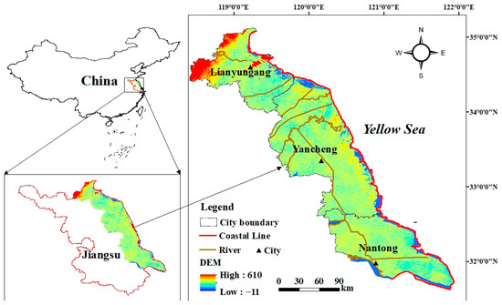
Figure 1.
The geographical location of the study area.
2.2. Data Sources and Preparation
Combined with previous research results, climate conditions, socioeconomic factors, and land use patterns were the major influencing factors of ecosystem services; their corresponding variables were selected as independent variables in the panel regression model [15,35,40]. In terms of the climate, the hydrothermal variation was a vital characterization of climatic conditions [24]. As Parmesan and Yohe (2003) pointed out, changes in temperature and precipitation patterns over time may have a large impact on ecosystem distribution and biophysical processes [41], so we selected two variables, average annual precipitation (APR) and average annual temperature (ATE). In terms of socioeconomic aspects, accelerated urbanization, population urbanization, economic urbanization, and land use urbanization have a greater impact on ESV temporal changes than climatic factors [42]. So, we selected population density (POP) and economic density (GDP) to represent the intensity of daily life and productive activities, respectively. In terms of land use patterns, land use intensity (LDI) can reflect changes in land use patterns, which can affect a variety of ecological processes and functions such as water quality, biodiversity, and vegetation carbon stocks. Therefore, we employed LDI to represent the land use factor and calculated it concerning Brentrup et al. (2002) [43]. The calculation formula is shown below.
represents the land use intensity score of the k-th research cell, n represents the total number of land use types in the study cell, represents the proportion of land use type i to the entire area of the study cell, and represents the pressure score of land use type i. Urban land is most affected by human daily and production activities, and we assigned the highest score of 10 to it, while cropland, woodland, grassland, water, and unused land were given scores of 6, 4, 2, and 0, respectively [44,45].
This paper used land use data (2000, 2005, 2010, 2015, and 2019) with a spatial resolution of 30 m × 30 m, obtained by interpreting Landsat TM/ETM and Landsat 8 remote sensing imagery. The data were obtained from the Data Center for Resource and Environmental Sciences, Chinese Academy of Sciences (http://www.resdc.cn/, accessed on 1 February 2022), which was widely adopted by many researchers in China [46,47]. Based on 30 m × 30 m precision land use/land cover data, we identified various ecosystem types in 2000, 2005, 2010, 2015, and 2019, and established a dataset of the spatial distribution of multi-cycle types of ecosystems in the study area, which included six types: cropland, woodland, grassland, water, bare land, and urban land. The data on climate impact factors APR and ATE were obtained from the National Earth System Science Data Center (http://www.geodata.cn/, accessed on 12 February 2022), and the data on socioeconomic impact factors POP and GDP were obtained from the Resources and Environment Science Data Center of the Chinese Academy of Sciences (https://www.resdc.cn/, accessed on 12 February 2022). The flow chart of this research process is shown in Figure 2.
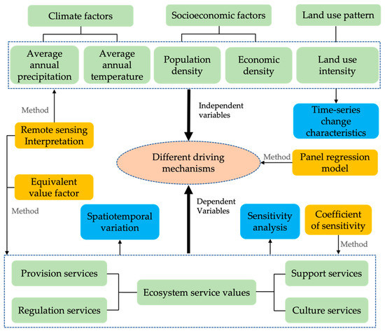
Figure 2.
Flow chart of the study.
2.3. Methods
2.3.1. Land Use Changes
The single land use dynamic degree provides a visual representation of the dynamics of land use types over the study period [48]. This study employs the single land use dynamic degree to measure the speed and magnitude of change in a land use type over a given period, which is formulated as follows:
where denotes the dynamic degree of each land use type. and refer to the area of a particular land use type at the start and the end of the study period, respectively. T represents the study period.
2.3.2. Accounting for ESV
Costanza (1997) was the first to propose a theoretical approach to ESV evaluation [1], which has received the attention of many researchers. Xie et al. (2008) adopted Costanza’s approach to constructing an ecosystem service value equivalent factor scale suitable for China based on the structural characteristics of Chinese ecosystems [16]. The ESV equivalent factor was based on the relative contribution of ecosystem services generated by different ecosystems and is approximately 1/7 of the average market value of food yields in the study area [20]. We modified the ESV equivalence coefficients to take the average grain yield and the average price of the region as the benchmark yield and price based on the actual situation in the Jiangsu coastal zone. The revised ESV equivalence factor for the study area was 2038.4 CNY/hm2, and we used it as the basis for calculating the ESV factor per unit area of the Jiangsu coastal zone (Table 1). The value of urban land was ignored in this study due to its low ESV.

Table 1.
ESV per unit area of different land use types in Jiangsu coastal zone (CNY/hm2).
We employed the equivalence coefficient method to calculate the ESV of various land use types based on their areas and finally obtained the total ESV of the Jiangsu coastal zone. The relevant formulas are as follows [49]:
where , , and denote the ESV of the j-th land use type, the ESV of the k-th ecosystem service function type and the total ecosystem service values, respectively. represents the area (hm2) of the j-th land use type and represents the value coefficient (CNY/hm2/year) for the k-th ecosystem service function type on the j-th land use type.
2.3.3. Sensitivity Analysis
To validate the reasonableness of the assessed ESV, a 50% adjustment was applied to the value coefficients (VC) for each land use type [34], and the sensitivity coefficient (CS) was employed to elucidate the extent to which the value coefficient affects the ESV at different time scales [50]. The CS can be expressed as follows:
where and are the initial and adjusted values of the ESV, respectively. and denote the initial and adjusted values of the ESV coefficient for the k-th land use type, respectively. When CS > 1, the elasticity of ESV relative to VC is high, meaning that the evaluation results are less credible, while the opposite is true when CS < 1. The bigger the percentage change in ESV relative to VC, the more important it is to use an accurate VC [51].
2.3.4. Spatial Heterogeneity of ESV
Spatial autocorrelation can be seen as a special correlation, a concept that defines the field of spatial analysis [52], and has been widely used in many modern fields after being introduced to spatial econometrics by Anselin [53]. To further analyze the spatial distribution characteristics of ESV and its variability in the Jiangsu coastal zone, we employed the global Moran’s I index, which was used to respond to the degree of correlation and variation between observations of spatially adjacent or nearby regional units across the study area [54]. The calculation formula is as follows.
denotes the number of ESV study units. denotes the observed value of the ESV study unit k(l). represents the spatial weight: 1 for spatial adjacency and 0 for non-adjacency. is the average value of the ESV study units. takes values in the range [−1,1]. When the value of is close to 1, there is an aggregation pattern for this indicator, a dispersion pattern when it is close to −1, and a random distribution pattern when it is close to 0.
2.3.5. Panel Regression Model
Panel data with both cross-sectional and temporal dimensions can significantly improve the accuracy of regression results [55] and are widely used in the analysis of influencing factors in economics, management, and other fields [56,57,58]. Therefore, this study constructed a panel data regression model to explore the driving mechanisms of regional ESV spatial and temporal heterogeneity. The basic setup of the econometric model is as follows:
Where denotes the dependent variable, being the total and different types of ESV of study cell i in period t. , , , , and represent independent variables. is a constant term and ~ are regression coefficients. indicates random disturbance term. The indicators in Equation (8) were subjected to logarithmic treatment for avoiding the effects of heteroskedasticity and inter-series cointegration.
3. Results
3.1. Land Use Dynamics Change
As can be seen from Figure 3 and Figure 4, land use changes in the Jiangsu coastal zone between 2000 and 2019 were significant. Cropland was always the dominant land cover type in the region, accounting for over 75% of the total land area, followed by urban land and water. Woodland, grassland, and bare land made up the smallest proportion, together accounting for less than 0.5%, which can be neglected. Cropland, urban land, and water were the main types of land use changes in the Jiangsu coastal zone during the last 20 years. The cropland area continuously declined by 1645.84 km2, and its proportion of the total land area decreased linearly from 81.99% in 2000 to 76.92% in 2019. The area of urban land consistently increased, by 2004.75 km2, and its share increased from 9.56% to 15.74%. The share of the water area increased from 8% to 8.78% and then gradually decreased to 7.1%, with a total reduction of 294.19 km2.
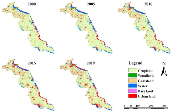
Figure 3.
Spatial distribution of land use types in the study area from 2000 to 2019.
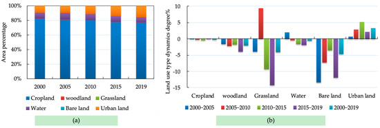
Figure 4.
Changes in the area structure (a) and dynamic degree of land use types (b) in the Jiangsu coastal zone.
The changes in land use dynamic degree (K) in Figure 3 revealed that the K value for urban land was positive, meaning that its area was continuously increasing between 2000 and 2019. K values were negative for cropland, woodland, and bare land. The K value for the water area was positive in 2000–2005 and became negative after that. The rapid progress of urbanization, especially the construction of the demonstration zone for undertaking industrial transfers in the Jiangsu coastal zone since 2010, has resulted in a significant decrease in cropland area and a substantial increase in the urban land area [59]. From 2000 to 2019, the K values were positive for all land types except for urban land which had negative values. The K values for woodland, grassland, and bare land were higher, but their absolute values were lower and therefore not the main land use types affecting ESV changes in the study area.
3.2. Spatiotemporal Variation of ESV
3.2.1. ESV Time Scale Variation
We evaluated the ESV by region for the years 2000 to 2019 based on the revised ESV coefficients, and the results are presented in Table 2 and Table 3. Overall, the total ESV of the Jiangsu coastal zone exhibited an inverted “V” shaped trend of increasing and then decreasing, which increased from CNY 676.65 × 10⁸ in 2000 to a maximum of CNY 693.72 × 10⁸ in 2005 and then began to decline to CNY 619.76 × 10⁸ in 2019. Total ESV decreased by CNY 56.89 × 10⁸ (8.41%) over the study period, with the most significant decrease of 4.93% occurring between 2010 and 2015. The structure of the ESV component indicated that the value share of cropland remained consistently above 60%, with the most considerable contribution to ESV, followed by water (34.37–37.99%). The sum value of woodland, grassland, and bare land accounted for no more than 1.5% of the total value.
Table 2.
ESV and its changes in ecosystem services for all land use types from 2000 to 2019.
Table 3.
Changes in the value of individual ecosystem functions in the Jiangsu coastal zone from 2000 to 2019.
The change in total ESV was negative (−233.75%), indicating a clear downward trend in ESV in the Jiangsu coastal zone between 2000 and 2019 (Table 2). The rate of change in ESV for cropland was −6.18%, which was closely related to the decrease in the share of cropland area from 81.99% in 2000 to 76.92% in 2019. While the change rate of the water area was −11.32%, its ESV decreased from CNY 240.21 × 10⁸ in 2000 to CNY 213.01 × 10⁸ in 2019. Woodland, grassland, and bare land have a small or even negligible impact on ESV due to their small size, even if they have significant change rates. Therefore, cropland and water areas were the main providers of ESV in the Jiangsu coastal area during the study period, and their area encroachment was also the main reason for the decline in ESV.
In terms of primary ecological service functions, the contribution rates of individual ecological services in the Jiangsu coastal zone from 2000–2019 were regulating services, supporting services, supply services, and cultural services, in descending order. They all exhibited different degrees of decreasing trends, with rates of −8.96%, −7.37%, −6.86%, and −10.42%, respectively (Table 3). Regulation services, cultural services, and support services exhibited a tendency of first increasing and then decreasing, with the maximum values occurring in 2005, while provision services presented a continuing trend of decrease. For secondary ecological services, waste treatment contributed the most (22.72–23.24%) followed by water regulation (20.66–21.82%), and the smallest was raw material (less than 4%). During the research period, the values of all secondary ecological service functions exhibited a general trend of relative decline, among which the values of food production, raw materials, gas regulation, and soil formation and conservation declined year by year, while the values of the other functions experienced an upward and then downward trend. The values of recreation culture and water supply suffered the largest decreases at 10.42% and 10.05%, respectively.
3.2.2. ESV Spatial Scale Variation
We used the natural breakpoint method of ArcGIS 10.2 software to divide the ESV results in the study area into five levels, forming a spatial pattern distribution of ESV per unit area for five time periods (Figure 5). There was significant spatial heterogeneity in ESV changes over 20 years. Extremely high and high ESV regions were mainly distributed in the Yellow Sea coastal and inland water network. Medium ESV areas were predominantly distributed on cropland and continued to shrink. The extremely low and low ESV regions were mainly located near the main urban areas or in urban settlements, with a wide distribution of urban land. Before 2010, the ESV was relatively little changed. After 2010, with the expansion of the transfer from the industries of Shanghai and southern Jiangsu and the continuous development of the Jiangsu coastline, the ESV began to decline on a large scale, with significant declines mainly in the coastline area, northeast of Lianyungang, central Yancheng and southwest of Nantong. Therefore, while developing the economy and the coastline, it is important to pay special attention to the impact on the ecological environment [37].
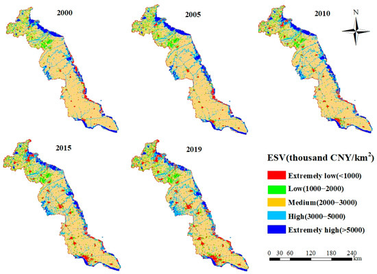
Figure 5.
Spatial distribution of ESV changes in the Jiangsu coastal zone from 2000 to 2019.
To explore the overall clustering characteristics of the spatial distribution of ESVs in the Jiangsu coastal zone, the global Moran’s I of ESVs in different periods was calculated using ArcGIS 10.2 software according to Equation (7). As can be seen from Table 4, the global of ESV for the five years in the Jiangsu coastal zone is greater than 0 and passes the significance test at the 1% level. The ESV exhibited a strong positive spatial correlation and displayed a more significant pattern of spatial clustering distribution in space. The value of the global fluctuated over the years but did not change much, increasing slightly from 2000 to 2005 and subsequently trending slowly downward, which suggested a relatively stable overall spatial agglomeration pattern.
Table 4.
Global spatial autocorrelation of ESV.
The hotspot detection revealed the spatial clustering characteristics of ESVs in the Jiangsu coastal zone from 2000 to 2019 (Figure 6). ESV spatial clustering was not significant in most parts of the study area, with the number of significant regional hotspots being bigger than the number of cold spots. The changes in cold spots were less pronounced from 2000 to 2010, and after 2010 the change in hotspots was less pronounced, while the number of high cold spots became more numerous and showed a tendency to be contiguous. In general, there were apparent zoning differences in ecosystem services in the Jiangsu coastal zone, with the coastal and riparian zones being the “main battlegrounds” for urbanization, and water bodies and cropland being the “logistical force” providing ecosystem service support [60].
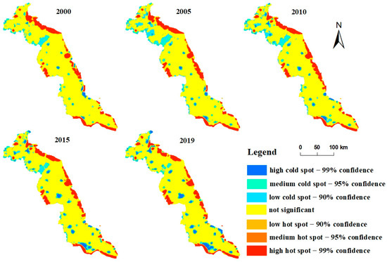
Figure 6.
Spatial clustering characteristics of ESV in the Jiangsu coastal zone from 2000 to 2019.
3.3. Sensitivity Analysis
The CS values for the Jiangsu coastal zone were calculated by adjusting the VC up or down by 50% according to Equation (6) (Table 5). The results indicated that the CS values varied considerably between land use types but less between years. The CS values for different land use types in five periods were all less than 1, with the highest CS value for cropland. The reason was that the proportion of cropland in the Jiangsu coastal zone was the largest, and the VC value of cropland was higher, so cropland had the greatest impact on ESV. The maximum CS value for cropland is 0.961, implying that when the VC of cropland increases by 1%, the ESV will increase by 0.961%. The CS value for the water rose from 0.432 to 0.469, and then gradually dropped to 0.415. The minimum CS values for grassland and unused land were 0.000. The CS values for each land use type during the study period were less than 1, indicating that the ESV of the Jiangsu coastal zone was inelastic with respect to the VC and that the modified equivalence factor was applicable to the study area.
Table 5.
The results of the CS for ESV in the Jiangsu coastal zone.
3.4. Driving Force Analysis
To improve the accuracy of spatial description and regression analysis, this paper divides the Jiangsu coastal zone into 5 km × 5 km scale grids, and each grid constitutes a study cell. When dividing the spatial grid purchase, there were many irregular cells with areas much smaller than 25 km generated at the edge of the study area. Therefore, this study draws on the processing methods of other scholars and includes only 1150 grids with an area larger than 20 km in the analysis of ESV impact mechanisms [61].
We employed box–line plots to analyze the intra-annual variability in the factors of climate change, socioeconomic, and land use patterns (Figure 7). The results showed that the economic density (GDP) has continued to grow in the past 20 years, with an increase rate of 654.3%. The overall fluctuation of population density (POP) is relatively small, featuring a concentration of population in individual areas. Climate changes were more evident, and the general trend of APR was not noticeable, while ATE decreased slightly before 2010 and increased significantly from 2010 to 2019, with an average increase of nearly 1 °C, which indicated a gradual warming trend in the Jiangsu coastal zone. The LDI declined from 2000 to 2005 and began to rise gradually and slowly after that, indicating that human exploitation of land resources had increased in recent years.
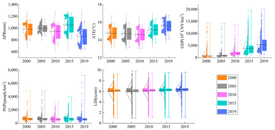
Figure 7.
Evolutionary characteristics of indicators of driving factors from 2000 to 2019. The sample size is 5750.
We applied Stata 15.0 software to perform econometric regression analysis on the constructed panel regression models. To guarantee the robustness of the model and the credibility of the regression results, we performed correlation tests such as multiple cointegrations, normal distribution, and serial unit root before regression analysis. Based on the results of the Hausman test, this study selected the panel random effects model to analyze the drivers of ecosystem services, and the results are shown in Table 6. Among them, model (1) explored the influence mechanism of total ESV, and models (2) to (4) analyzed the influence mechanisms of different ecosystem service functions, namely, provision services, regulation services, support services, and cultural services.
Table 6.
Regression results for driving factors of ESV in the Jiangsu coastal zone.
The regression results showed that for TOESV the effect of other drivers was significant, except for the insignificant effect of APR on ESV in the Jiangsu coastal zone. The regression coefficient of the average annual temperature (ATE) was significantly positive, indicating that the heat conditions provided by high temperatures contribute markedly to the enhancement of ecosystem services [60]. The regression coefficients for economic density (GDP) and population density (POP) were −0.013 and −0.095, respectively, revealing that socioeconomic factors have a significant inhibitory effect on the overall ecological environment and that high-intensity human living and production activities lead to a decrease in ESV [62]. Land use intensity (LDI) had a significant inhibitory effect on ESV improvement, with the most powerful impact among all factors. The reason may be that the dramatic change in land use type, especially the rapid expansion of urban land, directly or indirectly influences the regional socioeconomic and climatic characteristics [63]. Overall, land use patterns (LDI) and socioeconomic factors (GDP and POP) have a strong negative influence on ESV, while climate factors (APR and ATE) have a more positive influence on ESV, with LDI being the first driver, followed by ATE and then POP and GDP.
The regression results of models (2) to (4) suggested that significant heterogeneity existed in the drivers of different ecosystem service functions in the Jiangsu coastal zone. Land use patterns had varying degrees of negative effects on different types of ESVs and only showed a positive contribution to supply services. It may be that the proportion of cropland area in coastal areas of Jiangsu is above 70%, which contributes significantly to the increase in raw material (grain) production. Climatic hydrothermal conditions exerted a positive contribution to all types of ESV, although individual factors were not significant. In general, socioeconomic indicators (GDP and POP) had a significant inhibitory effect on different types of ESV, but the effect intensity differed significantly. Yet GDP promoted regulation services and cultural services, which were closely related to the development of tourism ecology driven by rapid economic growth, such as the increase in artificial lakes and planted forests, which were beneficial to both ecological regulation and aesthetic landscapes. Although there was variability in the degree of influence of drivers on different types of ESVs, on the whole, land use pattern was the first driver, followed by climate change and finally socioeconomic factors.
4. Discussion
4.1. Spatiotemporal Variability of the ESV
ESV is a tangible manifestation of the various ecosystem service functions provided by the natural environment and a key indicator of regional sustainable development [54]. With the transformation of land use type, the ecological pattern and function of the landscape also changed, which led to the variation in ecological space in the Jiangsu coastal zone. Between 2000 and 2019, the total ESV at the grid size of 1 km × 1 km first increased and then gradually decreased, with a total decrease of 8.41% (Table 2). Clusters of moderate ESV levels largely dominated their geographic distribution patterns, with higher ESV levels near waters along the coastal zone and lower ESV levels near towns and their peripheries. The main reason for the decline in total ESV is the shift from farmland and water types to urban land, leading to severe ecosystem decline and, thus, failure to provide adequate ecosystem services [33]. Meanwhile, altered land use types directly drive changes in biodiversity [44], further reducing the quantity and quality of services that ecosystems can continue to provide to human beings. For example, accelerated encroachment on wetlands due to regional population growth impedes the ability of wetlands to provide services such as hydrological regulation [39].
The coastal areas are characterized by relatively abundant water resources and a good ecological environment, but in recent years the ecological environment has been made sensitive due to the serious pollution imposed by developed industries. Ecological restoration policies, such as the “Jiangsu Province Wetland Protection and Restoration System Implementation Plan”, “Jiangsu Ecological River and Lake Action Plan”, and other documents issued by the Jiangsu government to promote the ecological civilization of wetlands, can limit the unreasonable development of land resources in its coastal areas and should be strengthened [64]. Urban land in the study area can reduce the ESV substantially due to its significantly lower contribution to ESV than other land types [47]. Therefore, rational land use planning is needed to slow down the rate of urban land expansion and encroachment on other land types through human intervention, which is essential for the enhancement of regional ecosystem services and macro balance and value transformation [35]. From the composition of ESV, regulating services contribute the most to ESV and are a crucial part of the increase or decrease in regional ESV, which coincides with the large watershed area of coastal areas and their high-value equivalent factor values. In summary, small changes in land use in the Jiangsu coastal zone can cause significant variations in ESV, indicating that the ESV is relatively sensitive to it. Therefore, in the future development of natural resources, it is necessary to focus on integrating socioeconomic and ecological resources, explore the optimal pattern of land resource use, and ultimately achieve a high level of collaborative ecological and economic development [60].
4.2. Key Drivers of Different Ecosystem Services
It is fundamental to ecosystem service management and decision-making to explore ecosystem services’ external spatial and temporal evolution and the mechanisms of their intrinsic impacts [6]. Ecosystem services and their value realization are influenced by multiple drivers, and their sensitivity to different drivers varies, which largely reflects the complexity of the mechanisms driving ecosystem services [63]. Land use change is primarily influenced by human activity and socioeconomic development, and the relationship with ESV generally has a significant dependency [65]. In this study, we found that the most noticeable changes from 2000 to 2019 in the Jiangsu coastal zone were the conversions of cropland and water to urban land (Figure 4), which significantly reduced the service capacity of ecosystems. Climatic conditions, such as precipitation and temperature, strongly influenced the composition, structure, and distribution of regional ecosystems, which had been proven to have a significant impact on ESVs [35,66]. In coastal areas, the impact of average annual temperature on ecosystem services is more intense, probably because the increase in evapotranspiration with higher temperatures drives water production and quality [46]. However, rising temperatures and falling precipitation may also bring about drought, further affecting the regional water cycle, raw material production, soil conservation, etc. [67]. Guo et al. pointed out that there were also significant synergistic and threshold effects of temperature and precipitation on ecosystem services, with higher temperatures inhibiting the ESV growth when evapotranspiration and precipitation were outside the threshold range, which meant that a mismatch between water and thermal conditions could have a dampening effect on ecosystem services [42,61]. It has been shown that there is a negative relationship between socioeconomic factors and ESVs in different regions or at different periods [18,24]. We demonstrated that socioeconomic factors, represented by economic density and population density, have a contradictory relationship with ESV, exerting a significant negative effect, and the inhibitory effect of population density is more substantial.
Ecosystem services have been classified into four broad categories: provisions, regulation, support, and cultural services, which is also the most widely adopted classification [4,7]. Previous studies have mainly analyzed the effects of different drivers on total ESV while neglecting their impact on different types of ESV. Comparing and analyzing the driving mechanisms of different kinds of ESVs is more helpful in grasping the root causes of ecosystem problems and guiding the construction of a regional ecological civilization [50]. Our study confirms that there are significant differences in the degree of influence of the same drivers on different types of ESVs, but the overall direction of influence is the same, with land use pattern as the first driver and climate change and socioeconomic factors ranking second and third, respectively. The Jiangsu coastal zone has the typical characteristics of coastal areas: abundant water resources, high temperatures, and rainy summers, where the regulatory services of the ecosystem play a leading role [39]. In addition, land use patterns have changed significantly, with urban expansion, agriculture, and aquaculture resulting in the fragmentation and even disappearance of many large patches of the natural landscape [38]. This paper clarifies the driving mechanisms of different types of ESVs in coastal areas, which can help policymakers properly understand the characteristics within coastal ecosystems and thus make rational decisions. For example, it is important to pay special attention to land management and climate change characteristics; to coordinate conflicts between watersheds, arable land, and urban land in a scientific and reasonable manner; and to guide human production and life toward ecological resource conservation and value-added development so as to achieve a harmonious development of economic growth and ecological conservation. Therefore, this paper’s findings have positive implications for other coastal areas.
4.3. Uncertainties and Further Work
The spatial and temporal variations in ESVs are driven by numerous influencing factors. The most typical influencing factors such as land use pattern, climate, and socioeconomic factors are selected in this paper, but soil, biological, and policy factors are not considered due to limitations in data availability. Meanwhile, topographic factors were discarded because they did not satisfy the panel data conditions. In future studies, appropriate methods should be actively applied to refine them. In addition, this paper explores the spatial and temporal evolution and driving mechanisms of ESVs in the Jiangsu coastal zone from the perspective of ESVs as a whole, and also analyzes the driving causes of different types of ESV changes. However, there is a lack of research on the trade-off synergistic relationship of ESVs, and the influence of the mutual synergistic effect of the drivers on ESVs is also neglected; the focus of future research is to dig deeper into the causes of ESV changes.
5. Conclusions
Humans living and producing have changed the natural environment, landscape patterns, and the ability of ecosystems to provide a variety of services under natural conditions in areas of high economic development and densely populated areas [33]. Therefore, the areas’ relationship with ESVs and their impacts on human well-being are of great interest [62]. In this paper, based on remote sensing data from 2000 to 2019, we evaluated the ESV in the Jiangsu coastal zone using the benefit transfer method and analyzed the spatial and temporal distribution characteristics of the ESV. Then, we constructed stochastic panel data models to quantify the driving mechanisms of influencing factors on different types of ESVs. The findings are as follows:
(1) From 2000 to 2019, land use types changed significantly, mainly concentrated in wetlands and urban fringes, with a significant reduction in cropland and water areas and a continued urban land expansion. This finding is consistent with the findings of Bao et al. (2019) [68]. The rates of other land type changes were higher but can be negligible owing to the small absolute area.
(2) The ESV provided by ecosystems in the Jiangsu coastal zone showed a trend of increasing and then decreasing, with a decrease of CNY 5.689 billion (8.41%) during the study period. Among them, the contributions of land use types and ecosystem service functions to ESV were as follows: farmland > watershed > forest land > grassland > unused and regulating services > support services > provisioning services > cultural services. The combined contribution of farmland and water exceeded 95%, and that of regulation and support services exceeded 80%.
(3) In the past 20 years, the distribution of ESVs in the study area showed prominent spatial variation characteristics, with hotspots mainly distributed near the coastal zone and cold spots distributed in towns and surrounding areas.
(4) The combined effects of land use patterns, climate variation, and socioeconomic factors contributed to the spatial variability of ESVs in the study area, and there were significant differences in the extent of their effects on different types of ESVs. Overall, land use intensity dominated ESV variation and was the first driver, followed by climate variation and socioeconomic factors. LDI and POP had significant negative impacts on the total ESV and different ESVs, while GDP had positive effects on RSESV and CSESV and negative effects on other ESVs. APR and ATE had positive effects, although the effects on individual types of ESVs were not significant.
This study deepens our understanding of the spatial and temporal variability of ESVs and their driving mechanisms in the Jiangsu coastal zone. The study results provide a new and useful reference method for the spatial and temporal analysis of coastal ecosystems, which is beneficial for promoting regional ecological civilization and sustainable development goals [59].
Author Contributions
Conceptualization, X.Z.; methodology, X.Z. and J.J.; software, X.Z.; validation, J.J.; formal analysis, X.Z.; investigation, J.J.; resources, X.Z. and J.J.; data curation, X.Z.; writing—original draft preparation, X.Z.; writing—review and editing, J.J.; visualization, X.Z.; supervision, J.J. All authors have read and agreed to the published version of the manuscript.
Funding
This research was funded by the National Social Science Foundation Key Projects of China, grant number 20AJL010, and the National Social Science Foundation Post-grant Project of China, grant number 19FGLB038.
Institutional Review Board Statement
Not applicable.
Informed Consent Statement
Not applicable.
Data Availability Statement
Not applicable.
Acknowledgments
The authors thank our colleagues and graduate students for their help in data collection and fieldwork. Special thanks to the editor and anonymous reviewers for their critical comments and valuable suggestions in the present form.
Conflicts of Interest
The authors declare no conflict of interest.
References
- Costanza, R.; d’Arge, R.; de Groot, R.; Farber, S.; Grasso, M.; Hannon, B.; Limburg, K.; Naeem, S.; Oneill, R.V.; Paruelo, J.; et al. The value of the world’s ecosystem services and natural capital. Nature 1997, 387, 253–260. [Google Scholar] [CrossRef]
- Bhardwaj, A.; Jasrotia, P.; Hamilton, S.; Robertson, G. Ecological management of intensively cropped agro-ecosystems improves soil quality with sustained productivity. Agric. Ecosyst. Environ. 2011, 140, 419–429. [Google Scholar] [CrossRef]
- Jantz, S.M.; Barker, B.; Brooks, T.M.; Chini, L.P.; Huang, Q.; Moore, R.M.; Noel, J.; Hurtt, G.C. Future habitat loss and extinctions driven by land-use change in biodiversity hotspots under four scenarios of climate-change mitigation. Conserv. Biol. 2015, 29, 1122–1131. [Google Scholar] [CrossRef]
- Cui, Y.; Lan, H.; Zhang, X.; He, Y. Confirmatory Analysis of the Effect of Socioeconomic Factors on Ecosystem Service Value Variation Based on the Structural Equation Model-A Case Study in Sichuan Province. Land 2022, 11, 483. [Google Scholar] [CrossRef]
- Zhao, Y.; Han, Z.; Xu, Y. Impact of Land Use/Cover Change on Ecosystem Service Value in Guangxi. Sustainability 2022, 14, 10867. [Google Scholar] [CrossRef]
- Cumming, G.S.; Buerkert, A.; Hoffmann, E.M.; Schlecht, E.; von Cramon-Taubadel, S.; Tscharntke, T. Implications of agricultural transitions and urbanization for ecosystem services. Nature 2014, 515, 50–57. [Google Scholar] [CrossRef]
- Costanza, R.; De Groot, R.; Sutton, P.; Van der Ploeg, S.; Anderson, S.J.; Kubiszewski, I.; Farber, S.; Turner, R.K. Changes in the global value of ecosystem services. Glob. Environ. Chang. 2014, 26, 152–158. [Google Scholar] [CrossRef]
- Bryan, B.A.; Ye, Y.; Zhang, J.E.; Connor, J.D. Land-use change impacts on ecosystem services value: Incorporating the scarcity effects of supply and demand dynamics. Ecosyst. Serv. 2018, 32, 144–157. [Google Scholar] [CrossRef]
- Costanza, R.; de Groot, R.; Braat, L.; Kubiszewski, I.; Fioramonti, L.; Sutton, P.; Farber, S.; Grasso, M. Twenty years of ecosystem services: How far have we come and how far do we still need to go? Ecosyst. Serv. 2017, 28, 1–16. [Google Scholar] [CrossRef]
- Wilkerson, M.L.; Mitchell, M.G.E.; Shanahan, D.; Wilson, K.A.; Ives, C.D.; Lovelock, C.E.; Rhodes, J.R. The role of socio-economic factors in planning and managing urban ecosystem services. Ecosyst. Serv. 2018, 31, 102–110. [Google Scholar] [CrossRef]
- He, B.J.; Zhao, D.X.; Gou, Z. Integration of Low-Carbon Eco-City, Green Campus and Green Building in China. Green Build. Dev. Ctries 2019, 31, 49–78. [Google Scholar]
- He, B.-J.; Zhao, D.-X.; Zhu, J.; Darko, A.; Gou, Z.-H. Promoting and implementing urban sustainability in China: An integration of sustainable initiatives at different urban scales. Habitat Int. 2018, 82, 83–93. [Google Scholar] [CrossRef]
- Li, J.; Chen, H.; Zhang, C.; Pan, T. Variations in ecosystem service value in response to land use/land cover changes in Central Asia from 1995-2035. PeerJ 2019, 7, e7665. [Google Scholar] [CrossRef] [PubMed]
- Arowolo, A.O.; Deng, X.; Olatunji, O.A.; Obayelu, A.E. Assessing changes in the value of ecosystem services in response to land-use/land-cover dynamics in Nigeria. Sci. Total Environ. 2018, 636, 597–609. [Google Scholar] [CrossRef]
- Woldeyohannes, A.; Cotter, M.; Biru, W.D.; Kelboro, G. Assessing Changes in Ecosystem Service Values over 1985–2050 in Response to Land Use and Land Cover Dynamics in Abaya-Chamo Basin, Southern Ethiopia. Land 2020, 9, 37. [Google Scholar] [CrossRef]
- Xie, G.; Zhen, L.; Lu, C. Expert knowledge based valuation method of ecosystem services in China. J. Nat. Resour. 2008, 23, 911–919. [Google Scholar]
- Chen, W.; Chi, G.; Li, J. Ecosystem Services and Their Driving Forces in the Middle Reaches of the Yangtze River Urban Agglomerations, China. Int. J. Environ. Res. Public Health 2020, 17, 3717. [Google Scholar] [CrossRef]
- Chen, W.; Zeng, J.; Zhong, M.; Pan, S. Coupling Analysis of Ecosystem Services Value and Economic Development in the Yangtze River Economic Belt: A Case Study in Hunan Province, China. Remote Sens. 2021, 13, 1552. [Google Scholar] [CrossRef]
- Li, F.; Zhang, S.; Yang, J.; Chang, L.; Yang, H.; Bu, K. Effects of land use change on ecosystem services value in West Jilin since the reform and opening of China. Ecosyst. Serv. 2018, 31, 12–20. [Google Scholar]
- Yu, Q.; Feng, C.-C.; Shi, Y.; Guo, L. Spatiotemporal interaction between ecosystem services and urbanization in China: Incorporating the scarcity effects. J. Clean. Prod. 2021, 317, 128392. [Google Scholar] [CrossRef]
- Piccolo, J.J.; Taylor, B.; Washington, H.; Kopnina, H.; Gray, J.; Alberro, H.; Orlikowska, E. “Nature’s contributions to people” and peoples’ moral obligations to nature. Biol. Conserv. 2022, 270, 109572. [Google Scholar] [CrossRef]
- Underwood, E.C.; Hollander, A.D.; Safford, H.D.; Kim, J.B.; Srivastava, L.; Drapek, R.J. The impacts of climate change on ecosystem services in southern California. Ecosyst. Serv. 2019, 39, 101008. [Google Scholar] [CrossRef]
- Moss, E.D.; Evans, D.M.; Atkins, J.P. Investigating the impacts of climate change on ecosystem services in UK agro-ecosystems: An application of the DPSIR framework. Land Use Policy 2021, 105, 105394. [Google Scholar] [CrossRef]
- Braun, D.; de Jong, R.; Schaepman, M.E.; Furrer, R.; Hein, L.; Kienast, F.; Damm, A. Ecosystem service change caused by climatological and non-climatological drivers: A Swiss case study. Ecol. Appl. 2019, 29, e01901. [Google Scholar] [CrossRef] [PubMed]
- Han, R.; Feng, C.-C.; Xu, N.; Guo, L. Spatial heterogeneous relationship between ecosystem services and human disturbances: A case study in Chuandong, China. Sci. Total Environ. 2020, 721, 137818. [Google Scholar] [CrossRef] [PubMed]
- Lawler, J.J.; Lewis, D.J.; Nelson, E.; Plantinga, A.J.; Polasky, S.; Withey, J.C.; Helmers, D.P.; Martinuzzi, S.; Pennington, D.; Radeloff, V.C. Projected land-use change impacts on ecosystem services in the United States. Proc. Natl. Acad. Sci. USA 2014, 111, 7492–7497. [Google Scholar] [CrossRef]
- Hasan, S.S.; Zhen, L.; Miah, M.G.; Ahamed, T.; Samie, A. Impact of land use change on ecosystem services: A review. Environ. Dev. 2020, 34, 100527. [Google Scholar] [CrossRef]
- Collin, M.L.; Melloul, A.J. Combined land-use and environmental factors for sustainable groundwater management. Urban Water 2001, 3, 229–237. [Google Scholar] [CrossRef]
- Xu, C.; Jiang, W.; Huang, Q.; Wang, Y. Ecosystem services response to rural-urban transitions in coastal and island cities: A comparison between Shenzhen and Hong Kong, China. J. Clean. Prod. 2020, 260, 121033. [Google Scholar] [CrossRef]
- Gashaw, T.; Tulu, T.; Argaw, M.; Worqlul, A.W.; Tolessa, T.; Kindu, M. Estimating the impacts of land use/land cover changes on Ecosystem Service Values: The case of the Andassa watershed in the Upper Blue Nile basin of Ethiopia. Ecosyst. Serv. 2018, 31, 219–228. [Google Scholar] [CrossRef]
- Guo, P.; Zhang, F.; Wang, H. The response of ecosystem service value to land use change in the middle and lower Yellow River: A case study of the Henan section. Ecol. Indic. 2022, 140, 109019. [Google Scholar] [CrossRef]
- Filho, W.L.; Barbir, J.; Sima, M.; Kalbus, A.; Nagy, G.J.; Paletta, A.; Villamizar, A.; Martinez, R.; Azeiteiro, U.M.; Pereira, M.J.; et al. Reviewing the role of ecosystems services in the sustainability of the urban environment: A multi-country analysis. J. Clean. Prod. 2020, 262, 121338. [Google Scholar] [CrossRef]
- Li, W.; Wang, L.; Yang, X.; Liang, T.; Zhang, Q.; Liao, X.; White, J.R.; Rinklebe, J. Interactive influences of meteorological and socioeconomic factors on ecosystem service values in a river basin with different geomorphic features. Sci. Total Environ. 2022, 829, 154595. [Google Scholar] [CrossRef] [PubMed]
- Li, K.; Wang, X.; Yao, L.; Shi, Y. Spatio-temporal change and driving factor analysis of ecosystem service value in the Beijing-Tianjin-Hebei region. J. Environ. Eng. Technol. 2021, 4, 1114–1122. [Google Scholar] [CrossRef]
- Pan, N.; Guan, Q.; Wang, Q.; Sun, Y.; Li, H.; Ma, Y. Spatial Differentiation and Driving Mechanisms in Ecosystem Service Value of Arid Region: A case study in the middle and lower reaches of Shule River Basin, NW China. J. Clean. Prod. 2021, 319, 128718. [Google Scholar] [CrossRef]
- Li, Z.; Xia, J.; Deng, X.; Yan, H. Multilevel modelling of impacts of human and natural factors on ecosystem services change in an oasis, Northwest China. Resour. Conserv. Recycl. 2021, 169, 105474. [Google Scholar] [CrossRef]
- Hoque, M.Z.; Islam, I.; Ahmed, M.; Hasan, S.S.; Prodhan, F.A. Spatio-temporal changes of land use land cover and ecosystem service values in coastal Bangladesh. Egypt. J. Remote Sens. Space Sci. 2022, 25, 173–180. [Google Scholar] [CrossRef]
- Huang, S.; Wang, Y.; Liu, R.; Jiang, Y.; Qie, L.; Pu, L. Identification of Land Use Function Bundles and Their Spatiotemporal Trade-Offs/Synergies: A Case Study in Jiangsu Coast, China. Land 2022, 11, 286. [Google Scholar] [CrossRef]
- Chuai, X.; Huang, X.; Wu, C.; Li, J.; Lu, Q.; Qi, X.; Zhang, M.; Zuo, T.; Lu, J. Land use and ecosystems services value changes and ecological land management in coastal Jiangsu, China. Habitat Int. 2016, 57, 164–174. [Google Scholar] [CrossRef]
- Redlich, S.; Zhang, J.; Benjamin, C.; Dhillon, M.S.; Englmeier, J.; Ewald, J.; Fricke, U.; Ganuza, C.; Haensel, M.; Hovestadt, T.; et al. Disentangling effects of climate and land use on biodiversity and ecosystem services-A multi-scale experimental design. Methods Ecol. Evol. 2022, 13, 514–527. [Google Scholar] [CrossRef]
- Parmesan, C.; Yohe, G. A globally coherent fingerprint of climate change impacts across natural systems. Nature 2003, 421, 37–42. [Google Scholar] [CrossRef] [PubMed]
- Guo, S.; Wu, C.; Wang, Y.; Qiu, G.; Zhu, D.; Niu, Q.; Qin, L. Threshold effect of ecosystem services in response to climate change, human activity and landscape pattern in the upper and middle Yellow River of China. Ecol. Indic. 2022, 136, 108603. [Google Scholar] [CrossRef]
- Brentrup, F.; Küsters, J.; Lammel, J.; Kuhlmann, H. Life Cycle Impact assessment of land use based on the hemeroby concept. Int. J. Life Cycle Assess. 2002, 7, 339. [Google Scholar] [CrossRef]
- Rüdisser, J.; Tasser, E.; Tappeiner, U. Distance to nature—A new biodiversity relevant environmental indicator set at the landscape level. Ecol. Indic. 2012, 15, 208–216. [Google Scholar] [CrossRef]
- He, Y.; Kuang, Y.; Zhao, Y.; Ruan, Z. Spatial Correlation between Ecosystem Services and Human Disturbances: A Case Study of the Guangdong–Hong Kong–Macao Greater Bay Area, China. Remote Sens. 2021, 13, 1174. [Google Scholar] [CrossRef]
- Fang, L.; Wang, L.; Chen, W.; Sun, J.; Cao, Q.; Wang, S.; Wang, L. Identifying the impacts of natural and human factors on ecosystem service in the Yangtze and Yellow River Basins. J. Clean. Prod. 2021, 314, 127995. [Google Scholar] [CrossRef]
- Xiao, R.; Lin, M.; Fei, X.; Li, Y.; Zhang, Z.; Meng, Q. Exploring the interactive coercing relationship between urbanization and ecosystem service value in the Shanghai-Hangzhou Bay Metropolitan Region. J. Clean. Prod. 2020, 253. [Google Scholar] [CrossRef]
- Wei, X.; Zhao, L.; Cheng, P.; Xie, M.; Wang, H. Spatial-Temporal Dynamic Evaluation of Ecosystem Service Value and Its Driving Mechanisms in China. Land 2022, 11, 1000. [Google Scholar] [CrossRef]
- Zhang, Z.; Gao, J.; Gao, Y. The influences of land use changes on the value of ecosystem services in Chaohu Lake Basin, China. Environ. Earth Sci. 2015, 74, 385–395. [Google Scholar] [CrossRef]
- Kreuter, U.P.; Harris, H.G.; Matlock, M.D.; Lacey, R.E. Change in ecosystem service values in the San Antonio area, Texas. Ecol. Econ. 2001, 39, 333–346. [Google Scholar] [CrossRef]
- Liu, Y.; Li, J.; Zhang, H.J.E.M. An ecosystem service valuation of land use change in Taiyuan City, China. Ecol. Model. 2012, 225, 127–132. [Google Scholar] [CrossRef]
- Getis, A. A history of the concept of spatial autocorrelation: A geographer’s perspective. Geogr. Anal. 2008, 40, 297–309. [Google Scholar] [CrossRef]
- Anselin, L. Spatial Econometrics: Methods and Models; Springer: Dordrecht, The Netherlands, 1988. [Google Scholar] [CrossRef]
- Moran, P.A.P. Notes on continuous stochastic phenomena. Biometrika 1950, 37, 17–23. [Google Scholar] [CrossRef] [PubMed]
- Alvarez, J.; Arellano, M. The time series and cross-section asymptotics of dynamic panel data estimators. Econometrica 2003, 71, 1121–1159. [Google Scholar] [CrossRef]
- Omri, A.; Kahouli, B. Causal relationships between energy consumption, foreign direct investment and economic growth: Fresh evidence from dynamic simultaneous-equations models. Energy Policy 2014, 67, 913–922. [Google Scholar] [CrossRef]
- Beenstock, M.; Felsenstein, D. Spatial error correction and cointegration in nonstationary panel data: Regional house prices in Israel. J. Geogr. Syst. 2010, 12, 189–206. [Google Scholar] [CrossRef]
- Fitrianto, A.; Musakkal, N.F.K. Panel Data Analysis for Sabah Construction Industries: Choosing the Best Model. In Proceedings of the 7th International Economics and Business Management Conference (IEBMC), Kuantan, Malaysia, 5–6 October 2016; pp. 241–248. [Google Scholar]
- Zhou, Y.; Ning, L.; Bai, X. Spatial and temporal changes of human disturbances and their effects on landscape patterns in the Jiangsu coastal zone, China. Ecol. Indic. 2018, 93, 111–122. [Google Scholar] [CrossRef]
- Liu, Z.; Wang, S.; Fang, C. Spatiotemporal evolution and influencing mechanism of ecosystem service value in the Guangdong-Hong Kong-Macao Greater Bay Area. Acta Geogr. Sin. 2021, 76, 2798–2810. [Google Scholar]
- Liu, Z.; Wu, R.; Chen, Y.; Fang, C.; Wang, S. Factors of ecosystem service values in a fast-developing region in China: Insights from the joint impacts of human activities and natural conditions. J. Clean. Prod. 2021, 297, 12588. [Google Scholar] [CrossRef]
- Liu, J.; Chen, L.; Yang, Z.; Zhao, Y.; Zhang, X. Unraveling the Spatio-Temporal Relationship between Ecosystem Services and Socioeconomic Development in Dabie Mountain Area over the Last 10 years. Remote Sens. 2022, 14, 1059. [Google Scholar] [CrossRef]
- He, Z.; Shang, X.; Zhang, T.; Yun, J. Coupled regulatory mechanisms and synergy/trade-off strategies of human activity and climate change on ecosystem service value in the loess hilly fragile region of northern Shaanxi, China. Ecol. Indic. 2022, 143, 109325. [Google Scholar] [CrossRef]
- Wu, C.; Chen, B.; Huang, X.; Wei, Y.H.D. Effect of land-use change and optimization on the ecosystem service values of Jiangsu province, China. Ecol. Indic. 2020, 117, 106507. [Google Scholar] [CrossRef]
- Yang, L.; Jiao, H. Spatiotemporal Changes in Ecosystem Services Value and Its Driving Factors in the Karst Region of China. Sustainability 2022, 14, 6695. [Google Scholar] [CrossRef]
- Markkula, I.; Turunen, M.; Rasmus, S. A review of climate change impacts on the ecosystem services in the Saami Homeland in Finland. Sci. Total Environ. 2019, 692, 1070–1085. [Google Scholar] [CrossRef] [PubMed]
- Ma, S.; Wang, L.-J.; Jiang, J.; Chu, L.; Zhang, J.-C. Threshold effect of ecosystem services in response to climate change and vegetation coverage change in the Qinghai-Tibet Plateau ecological shelter. J. Clean. Prod. 2021, 318, 128592. [Google Scholar] [CrossRef]
- Bao, J.; Gao, S.; Ge, J. Dynamic land use and its policy in response to environmental and social-economic changes in China: A case study of the Jiangsu coast (1750–2015). Land Use Policy 2019, 82, 169–180. [Google Scholar] [CrossRef]


Publisher’s Note: MDPI stays neutral with regard to jurisdictional claims in published maps and institutional affiliations. |
© 2022 by the authors. Licensee MDPI, Basel, Switzerland. This article is an open access article distributed under the terms and conditions of the Creative Commons Attribution (CC BY) license (https://creativecommons.org/licenses/by/4.0/).