Optimal Structuring of Investments in Electricity Generation Projects in Colombia with Non-Conventional Energy Sources

Abstract

Taking full advantage of fiscal and economic incentives has become a complex process for investors, who must find the right portfolio or capital structure to obtain viable and competitive generation projects. In this context, this paper proposes a methodology for the optimal structuring of investments in non-conventional energy sources (NCRES) considering fiscal and economic incentives. Three methods were evaluated: (1) levelized cost of electricity (LCOE) combined with three metaheuristic techniques; (2) discounted cash flow (DCF) with Monte Carlo simulation and value at risk (VaR); and (3) real options with Black and Scholes. The proposed approach presents as the main financial indicator the generation cost (GC), as well as three other financial indicators, namely: net present value (NPV), value at risk (VaR) and net present value for real options (NPV${}_{RO}$). The propose approach allows for defining different investment portfolios from where an investor can choose; each of which minimizes the GC. Furthermore, the methodology can be adapted to countries with different policies and fiscal incentives for the development of NCRES projects. The results show that for each metaheuristic, an optimal capital structure that minimizes GC is obtained; in this way, a GC of 0.032 (USD/kWh) is achieved for solar photovoltaic technology, with a reduction of 49.2%, when tax incentives are considered.

1. Introduction

The structuring of projects with non-conventional energy sources (NCES) represents a complex process for investors, who must define an adequate methodology to reduce or minimize generation costs (GC) under a local context of fiscal and economic incentives. Thus, it is necessary to establish investment strategies, through the use of financial and optimization methods, that allow determining the most appropriate generation technologies, considering issues such as intermittent, limited, or inefficient energy supply for rural and non-interconnected areas, lack of employment, low agricultural technification and lack of telecommunication services and modern infrastructure for the execution of daily activities, as well as low adaptation to climate change [1,2,3].

In China, for example, the authors in [4] adopted the Richardson maturity model (RMM) to evaluate the effect of credit period on the efficiency of non-conventional renewable energy source (NCRES) project investments. They conclude that it is necessary to define financial policies from the government and the banking system in order to support the development of companies dedicated to the implementation of NCRES projects. In [5], the authors conducted a literature review on the real options (RO) method for NCRES investments; in addition, they proposed some methodologies to promote the development of investments, such as heterogeneity of investors, segmentation policies, linking design and operation to investment processes, as well as the inclusion of vertical and horizontal analysis to evaluate investments. In [6], they used a semi-parametric regression model (SRM) to evaluate the impact of government subsidies, green credits, and environmental taxes on NCRES investments. The authors in [7], employed an analytic network process (ANP) to assess the risks of investments in renewable energy projects.

In Iran, the authors in [8], minimized the GC from the optimal selection of equipment topologies of a wind plant; to do this, they combined the levelized cost of electricity (LCOE) method with a genetic algorithm (GA). In Serbia, the authors in [9], presented the combination of the LCOE with a GA to minimize the GC from the technical specifications of different types of turbines for a wind plant. In Morocco, the authors in [10], used the response surface methodology (RSM), an artificial neural network (ANN), and the LCOE to minimize the GC of a solar photovoltaic plant from the irradiance and performance characteristics of the solar panels. In India, the authors in [11] minimized the GC of a hybrid renewable energy system composed of four generation technologies: solar photovoltaic, wind power, diesel generator, and batteries. In this case, in order to find the optimal hybrid topology to minimize the GC, the authors used three metaheuristic techniques: political optimizer (PO), particle swarm optimization (PSO), and interior point algorithm (IPA). In Korea, the authors in [12] proposed a network optimization model using mixed integer linear programming (MILP) to determine the optimal generation configuration and the time in which the investment should be made. In Qatar, the authors in [13] carried out a literature review on incentives and existing strategies for the financing of NCRES. They conclude that there are difficulties for the energy transition due to the unwillingness of governments and financial entities to encourage the NCRES through different policies, such as economic incentives for new generation technologies, soft loans, technological support, and disclosure about the advantages that NCRES present compared to other energy sources, such as oil.

The authors in [14] developed a financial methodology called Market Penetration Modeling of Renewable Energy Technologies in Electric Power Sector to assess the effects of economic incentives and the price of coal on the development of the NCRES projects. The methodology considers the least squares method (LSM), with which the electricity demand model of Canada is represented. The results indicate that an economic subsidy for each new kW of installed capacity and MWh generated, from NCRES, can promote the diversification of the energy matrix and the reduction of thermal power plants, which would cause a decrease in greenhouse gas emissions in the long term. In Brazil, The authors in [15], used topology optimization (TO) and the LCOE approach to minimize the GC of a photovoltaic solar plant based on a new metric that corresponds to the relationship between the annual energy produced and the area occupied by the solar panels. In Chile, the authors in [16], constructed a sensitivity analysis of the GC through multi-objective optimization (MO), which considered variations in the discount rate, initial investment, plant factor, payment for power, and operation term. These variations were performed independently within the LCOE model to determine the variation of the generation cost versus each variable. In Cuba, the authors in [17], conducted a study of investments in NCRES, based on a multi-criteria evaluation. The authors concluded that the method is suitable for analyzing the viability of projects under scenarios of social, environmental, and economic sustainability since it combines the quantitative and qualitative elements of the investments.

In Colombia, with the entry into force of the benefits of Law 1715 of 2014, Law 1955 of 2019, Law 2099 of 2021 and the reliability charge, NCRES projects are able to compete with conventional energy sources (CES) and have lower generation costs. The authors in [18] analyzed the potential effects of Law 1715 on electricity generation projects with NCRES; additionally, they included the tax incentives of the Law in the LCOE method to estimate the reduction of GC. The results showed that GC can be reduced by up to $20\%$.

The authors in [19] used the LCOE to analyze the effects of tax incentives of Law 1715 on the GC of forest biomass power cogeneration plants in the department of Antioquia, in Colombia. The results of the analysis showed that GC can be reduced by $11.2\%$ when incentives with 10-year asset depreciation, $50\%$ financing of the initial investment, and 5-year grace period are applied. In [20], the authors evaluated the effect of tax incentives of Law 1715 and Law 1955 on the levelized cost of energy of syngas using the LCOE approach. The authors considered a positive externality of revenues from the disposal of municipal solid waste. The authors in [21] analyze the effect of fiscal and economic incentives on electricity generation from urban solid waste (USW), using the LCOE method; the results obtained show that the GC is reduced by 37.4%, when considering a 100% debt, 70% in bank loans, and 30% in green bonds, and income from USW disposal and reliability charge. The authors in [22] evaluated the effect of debt on the levelized cost of substitute gaseous fuel produced from USW gasification; they used the LCOE method, finding that the cost of gaseous fuel decreases to a greater extent when tax incentives are applied with a debt grace period of 5 years.

The LCOE approach is used in [23] to estimate the GC of large-scale solar plants in Colombia, considering the fiscal benefits of Law 1715. In addition, the authors performed a deterministic sensitivity analysis using the weighted average cost of capital (WACC), energy produced, operation and maintenance expenses, as well as investment costs in order to facilitate investor’s decisions.

In [24], the RO method is employed to economically value wind farms and determine the appropriate timing of investments considering incentives. The authors in [25] proposed a hybrid method to select the most appropriate technologies for low-cost self-generation in shopping malls in Colombia, considering technical, technological, environmental, economic, and regulatory criteria. A financial analysis is conducted in [26] using the total cost and learning curve model in order to evaluate the economic impact of the integration of renewable energies in the Colombian electricity system. The results showed the feasibility of new generation technologies for the country, taking into account the current incentives.

The authors in [27] analyzed the problem of investments under uncertainty in power generation projects by developing a methodology based on volatility models, such as the generalized autoregressive conditional heterocedastic (GARCH) model and the autoregressive integrated moving average exogenous variables (ARIMAX) model. This methodology serves as an input to stochastically estimate the value at risk (VaR) of the cash flows of electricity projects. The authors in [28] presented an application of Black Litterman’s model considering seasonal autoregressive integrated moving average (SARIMA) and autoregressive conditional heteroscedasticity (ARCH) models to identify the behavior of the variables that determine the revenues and outflows of small hydroelectric power plants. The authors in [29] proposed a valuation of financial risk in the process of selling electricity through long-term contracts, using the Monte Carlo simulation method, value at risk (VaR), and conditional value at risk (CvaR).

In summary, the authors cited above use different methodologies to assess electricity generation projects based on NCRES considering technical and financial criteria. For example, in [9,10,11,15], the authors minimize the GC through the use of optimization techniques (ANN, RSM, GA, PO, PSO, IPA, and TO) applied to the LCOE approach. In this case, the decision also relies on technical variables of the NCRES, such as size, site location, materials, efficiency, and useful life of the technologies, among others. In contrast, this work applies three metaheuristic techniques, namely, GA, PSO, and differential evolution (DE) to the LCOE approach to minimize GC considering financial variables; furthermore, three additional financial indicators are used to value investments in NCRES under uncertainty scenarios: NPV, VaR, and NPV${}_{OR}$.

Table 1. Features of other methodologies and the proposed approach.

Reference	LCOE	OR	Other Methodologies	Optimization Techniques
[16]	Yes	No	No	MO
[8]	Yes	No	No	GA
[10]	Yes	No	No	ANN, RSM
[9]	Yes	No	No	GA
[11]	Yes	No	No	PO, PSO, IPA
[15]	Yes	No	No	TO
[19,20,21,22,23,24,25,26,27,28,29,30]	Yes	No	No	No
[5]	No	Yes	Vertical and horizontal analysis	No
[31]	Yes	No	No	No
[18]	Yes	No	No	No
[25]	Yes	Yes	AHP, Monte Carlo simulation and discounted flow cash	TOPSIS
[26]	No	No	Total Cost and Learning Curve	No
[24]	No	Yes	Discounted Cash Flow	No
Proposed	Yes	Yes	Discounted cash flow with Monte Carlo simulation and VaR	GA, PSO, DE

presents a comparative with other research works and how a knowledge gap is covered by the proposed methodology, where TOPSIS and AHP mean Technique for Order of Preference by Similarity to Ideal Solution and Analytic Hierarchy Process, respectively. It should be clarified that this work does not consider decision variables related to technical issues of the NCRES, but variables related to the financial part.

In the literature survey carried out by the authors, no methodology was found to optimally structure electricity generation investments with NCRES by combining values associated with five financial decision variables as proposed in this paper. The variables considered for the optimal investment portfolio are: (1) percentage of equity capital (${\alpha }_1$), (2) percentage of debt (${\alpha }_2$), (3) number of years for accelerated asset depreciation (d), (4) debt grace period (k), and (5) debt term (L). Thus, the combination given by these variables (${\alpha }_1$, ${\alpha }_2$, d, k, L) allows minimizing the GC by taking advantage of tax and economic incentives, as well as debt, which helps to reduce the effective tax rate of a project.

In summary, the main features and contributions of this paper are as follows:

• The use and comparison of three metaheuristic techniques applied to the LCOE method. This makes it possible to define a different investment portfolio for each metaheuristic technique that minimizes GC, providing the investor with several investment alternatives.
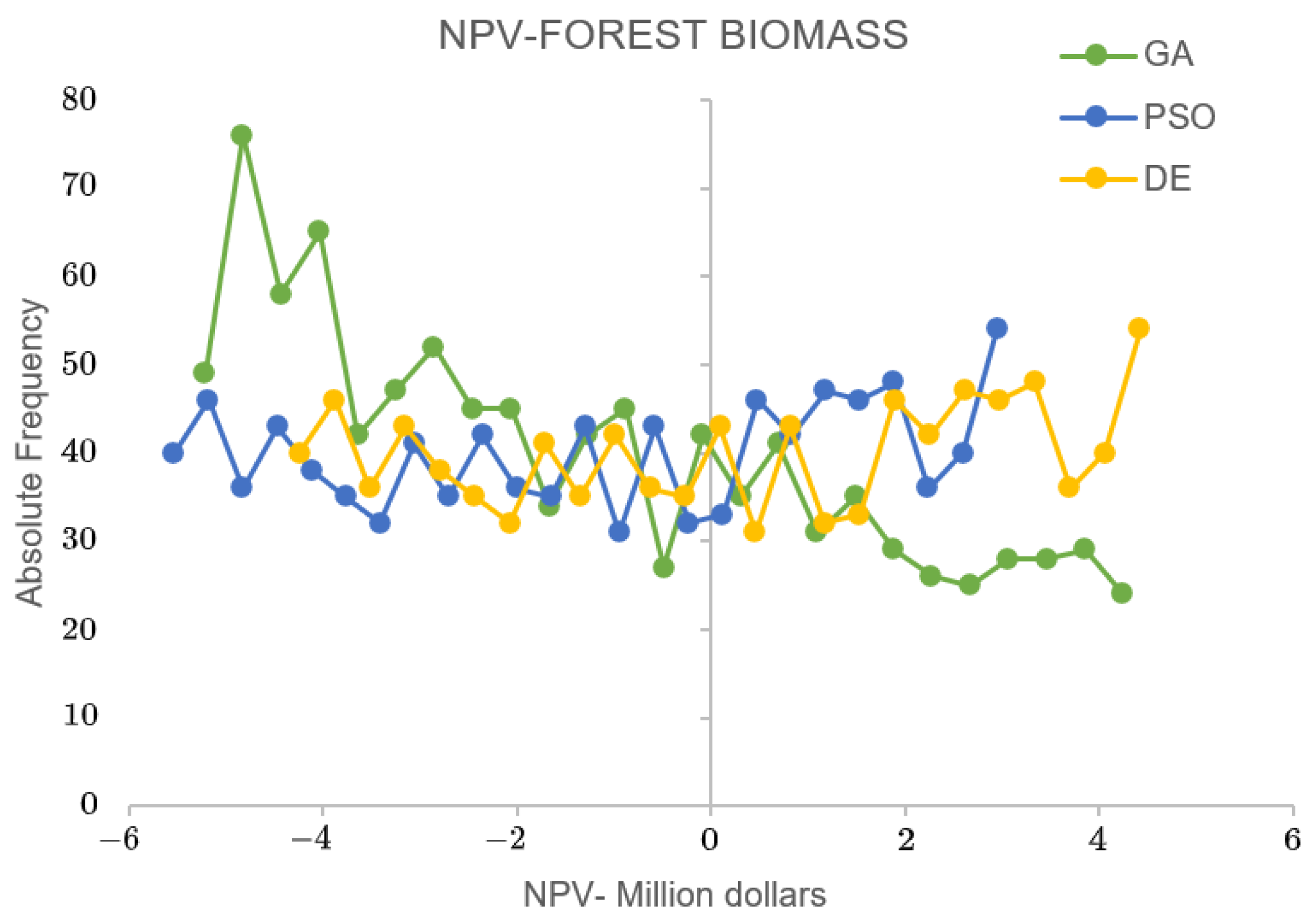
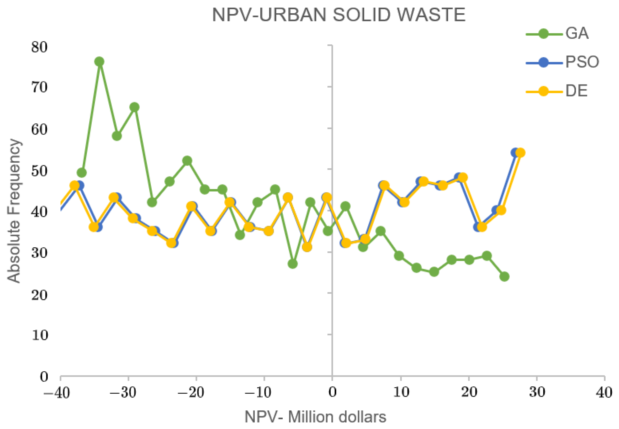
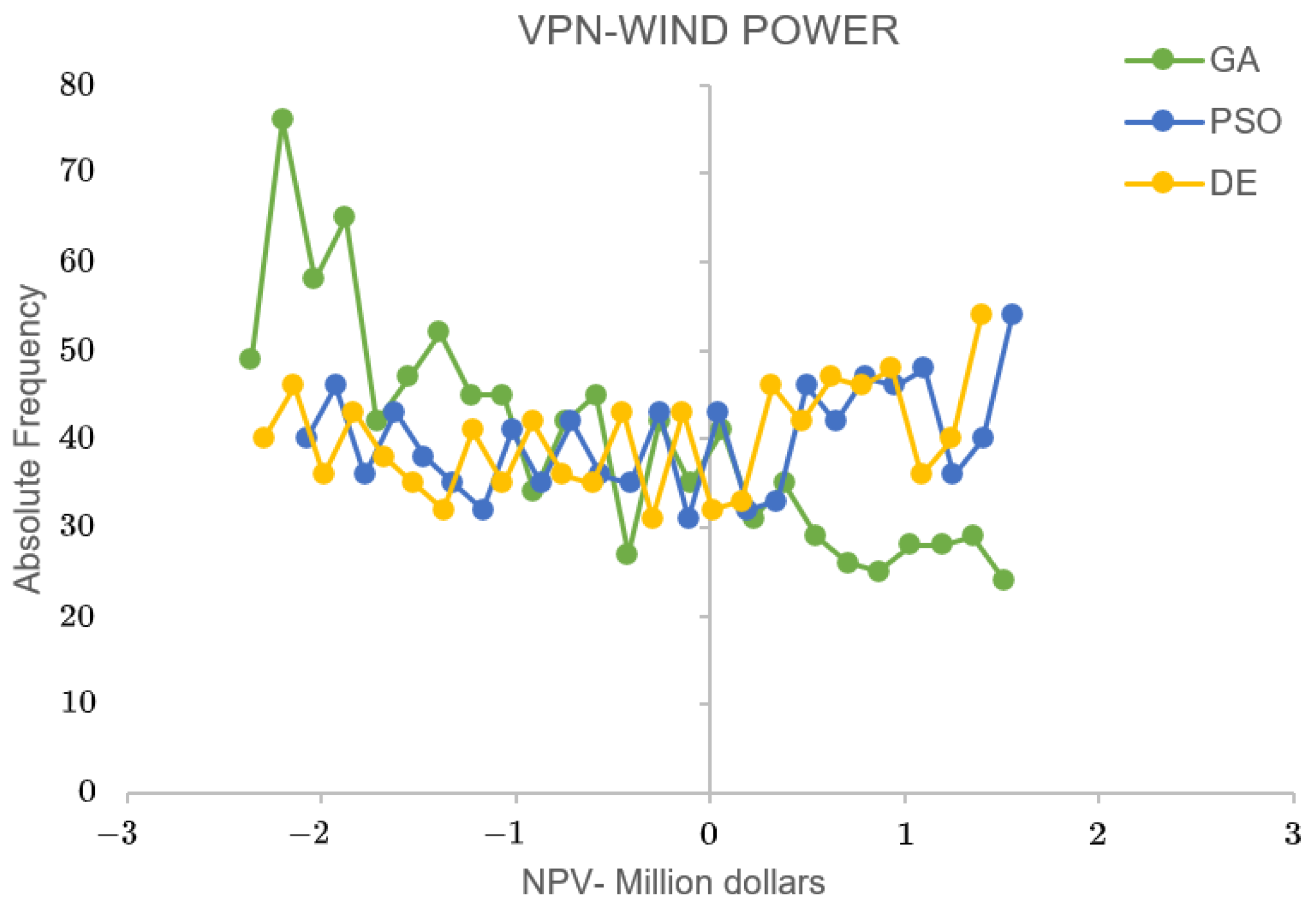
• Implementation of two risk assessment methods for NCRES investments, taking as reference the optimal portfolios and minimum GC (USD/kWh) calculated with the metaheuristic techniques and the LCOE. These methods are: (1) DCF method with Monte Carlo simulation and VaR, whose financial indicators are NPV(MUSD) and VaR (MUSD), respectively; and (2) RO method with Black and Scholes, whose financial indicator is NPV${}_{RO}$ (MUSD).
• The integration of aforementioned approaches to assess NCRES projects within an iterative methodology that provides potential investors with a set of decision options.
• The proposal of fiscal and economic incentives to make NCRES electricity generation projects viable. In this case, four technologies were considered: forest biomass (FB), urban solid waste (USW), solar photovoltaic (PV), and wind power (WP).

Although the proposed approach was envisaged within the Colombian context, it can be adapted and applied in other countries with different policies and fiscal incentives. The rest of the document is organized as follows: Section 2 details the three financial methods and metaheuristic techniques applied for optimal structuring of investments in NCES. Section 3 presents the results of the proposed approach. Section 4 presents some recommendations for the proposed methodologies to have a greater impact on the development of projects involving NCES. Finally, the conclusions of the research are presented in Section 5.

2. Methodology

Three financial methods (LCOE, DCF with Monte Carlo simulation and VaR, and OR with Black and Scholes) and three metaheuristic techniques (GA, PSO, DE) were considered for the optimal structuring of investments in NCES projects for electricity generation considering tax incentives.

2.1. Levelized Cost of Electricity and Tax Incentives in Colombia

The LCOE method is defined as the constant price (LCOE-USD/kWh) at which electricity must be sold to obtain an NPV of zero, during the project’s operating life. The LCOE considers the initial investment, fixed and variable administration, operation and maintenance (AOM) costs, fuel cost, reliability charge, positive and negative externalities, capital sources, green bonds, as well as fiscal and economic incentives, among others. Equation (1) shows the structure of the LCOE [30,32].

$$LCOE={\mathrm{LCOE}}_I+{\mathrm{LCOE}}_V+{\mathrm{LCOE}}_F+{\mathrm{LCOE}}_{FL}+/-{\mathrm{LCOE}}_E$$

(1)

where LCOE${}_I$ is the investment component per unit of energy (USD/kWh), which includes the costs associated with the acquisition of goods and services required for the design, construction and start-up of the project. LCOE${}_V$ is the AOM variable cost component per unit of energy (USD/kWh) and LCOE${}_F$ is the AOM fixed cost component per unit of energy (USD/kWh). This includes the costs associated with the services necessary to guarantee the operation and useful life of the project, such as hiring qualified personnel, goods and services for maintenance, payment of taxes and interest on debt, among others. It should be noted that variable costs vary according to the project’s production. LCOE${}_{FL}$ is the fuel cost component per unit of energy (USD/kWh), which includes the expenses caused by the acquisition of raw materials, from which the primary energy potential for electricity generation is obtained. LCOE${}_E$ is the externality component per unit of energy (USD/kWh), which can be negative (cost) or positive (income), depending on the environmental and social impacts of the project. In this work, only a positive externality was considered for USW technology, where an income is obtained from the disposition of USW to generate energy. It should be clarified that each component of the LCOE represents a percentage of the price at which the energy should be sold. Finally, Equation (2) presents the general expression for the LCOE, while Equation (3) includes tax, debt, and economic incentives within the LCOE.

$$\mathrm{LCOE}=\frac{I_o+{\sum }_{t=1}^n\frac{Ct}{{(1+i)}^t}}{{\sum }_{t=1}^n\frac{Et}{{(1+i)}^t}}$$

(2)

where $Io$ is the initial investment cost (USD), considered in the LCOE${}_I$ component of the LCOE; $Ct$ is the annual operating costs (USD), which includes fixed and variable AOM costs, fuel, and positive and negative externaties in components LCOE${}_V$, LCOE${}_F$, LCOE${}_{FL}$, and LCOE${}_E$ of the LCOE, respectively; $Et$ is the amount of energy produced in one year (kWh), i is the discount rate, n is the operational lifetime (years), and t is the useful life of the project (years) [1].

In 2014, the Colombian Congress approved the Law 1715 on Renewable Energies, which encourages investment in NCERS projects through four tax incentives, which are described as follows: (1) investors may annually reduce from their income, for 5 years following the taxable year in which they made the investment, $50\%$ of the total value of the investment made (Investment tax credit—ITC); (2) value-added tax (VAT) exemption for national or imported equipment, elements, machinery, and services used for the pre-investment and investment of the NCERS project; (3) exemption from the payment of tariffs for the aforementioned elements; (4) accelerated depreciation of assets, which will not exceed $20\%$ per year as a global rate [30].

In 2019, the government issued the National Development Plan 2018–2022, Law 1955 of 2019, which modifies one of the incentives of Law 1715 of 2014, the ITC. This benefit will be valid for 15 years and not 5, as initially proposed [30]. Finally, the government issued the Energy Transition Law, Law 2099 of 2021, which provides further incentives for the development of renewable energy projects in Colombia, increasing the overall annual depreciation rate to $33.33\%$.

Equation (3) corresponds to a modification of Equation (2) to explicitly consider two sources of financing, namely, debt and equity. It also considers the tax incentives in Colombia [30]. Additionally, Equation (3) represents the objective function (minimization of the LCOE) for the application of metaheuristic techniques to find the optimal investment portfolio, according to the capital structure of the project. Equation (4) represents the fiscal factor of the project during its operating life, and Equations (5)–(12) represent the OF constraints. It should be clarified that Equation (5) refers to the ITC.

$$\mathrm{LCOE}=\frac{1}{\mu {\sum }_{t=1}^n\frac{E_t}{{(1+i)}^t}}\left[{\alpha }_{1}I+\sum _{t=k}^{1+k}\frac{{\alpha }_{2}I{(1+g)}^k+\mu i_{D}L}{L{(1+E)}^t{(1+i)}^{{}^t}}+\sum _{t=1}^n\frac{\mu C_t}{{(1+i)}^t}+\sum _{t=1}^d\frac{D_{j}I}{{(1+E)}^t{(1+i)}^t}(\mu -1)\right]$$

(3)

$$\mu =1-\left(1-\sum _{t=1}^p{I}_t\right)\beta$$

(4)

Subject to:

$$\sum _{t=1}^p{I}_t\le 50\%$$

(5)

$$0\le p\le 15$$

(6)

$$0\%\le {\alpha }_1\le 100\%$$

(7)

$$0\%\le {\alpha }_2\le 100\%$$

(8)

$${\alpha }_1+{\alpha }_2=100\%$$

(9)

$$K,L\ge 0$$

(10)

$$0\le K+L\le n$$

(11)

$$3\le D_j\le 10$$

(12)

In this case, $\mu$ is the tax and incentive factor; $\beta$ is the tax rate ($35\%$); $I_t$ is the ITC rate; p is the maximum ITC utilization period in years (maximum 15 years); n is the operational lifetime of the project (20 years); t the useful life of the project (20 years); $E_t$ is the annual amount of energy produced (kWh); I is the initial investment cost (USD); ${\alpha }_1$ is the weight of equity capital (0–100%, dimensionless); ${\alpha }_2$ is the weight of debt (0–100%, dimensionless); i is the discount rate or cost of capital ($8.1\%$ A.E.); k is the grace period of the debt (years); L is the term of the debt (years); g is the interest rate of the debt ($6.56\%$ A.E.), as of 31 December 2021 [33]; $i_D$ is the annual interest on the debt (USD); E is the inflation rate ($5.62\%$ A.E.) [34], which corresponds to that accumulated for the year 2021 in Colombia; $C_t$ represents the sum of revenues from positive externalities and reliability charge, as well as annual project costs for administration, operation, maintenance, and fuel (USD); $D_j$ is the asset depreciation rate (≤33.33% A.E.); d is the time applied to asset depreciation (3–10 years) [30]. In this case, the decision variables are ${\alpha }_1$, ${\alpha }_2$, d, k, and L.

2.2. Discounted Cash Flow with Monte Carlo and VaR Simulation

Discounted cash flow (DCF) allows the net present value of a project to be calculated from the income and expenses incurred during its operating life. In this way, future cash flows are brought to present value using the investor’s discount rate and finally summed to obtain the net present value. Equation (13) shows the generalized expression of net present value using DCF [35].

$$\mathrm{NPV}=\sum _{t=0}^n\frac{(F_j+F_c)}{{(1+i)}^t}$$

(13)

where NPV is the net present value, $F_i$ is the income for year n of the cash flow (USD), $F_c$ is the expenditure for year n of the cash flow (USD), i is the discount rate ($8.1\%$ A.E.), n is the operational life of the project (years), and t is the useful life of the project (years).

Equation (14) shows the expression of the DCF for electricity generation projects with NCES, considering tax incentives and investment structure, which was adapted from Equations (3)–(6).

$$\mathrm{NPV}=\mu \mathrm{LCOE}\sum _{t=1}^n\frac{E_t}{{(1+i)}^t}\left[{\alpha }_{1}I+\sum _{t=k}^{1+k}\frac{{\alpha }_{2}I{(1+g)}^k+\mu i_D}{{(1+E)}^t{(1+i)}^{{}^t}}+\sum _{t=1}^n\frac{\mu C_t}{{(1+i)}^t}+\sum _{t=1}^d\frac{D_{j}I}{{(1+E)}^t{(1+i)}^t}(\mu -1)\right]$$

(14)

On the other hand, Monte Carlo simulation is a statistical tool that allows to evaluate the variability of the NPV when there is uncertainty in any variable of the DCF [36]. In this work, the Monte Carlo simulation was adapted to Equation (14) in order to obtain the different NPV that can be achieved when the representative market rate (RMR) is modified. Although the RMR is not explicitly found in Equation (14), its variation directly affects variable I, which corresponds to the value of the initial investment of a project. Furthermore, the increase or decrease of I causes the capital structure of a project to be modified due to changes in the value of the debt, its term and grace period, as well as the overall annual rate of accelerated depreciation of assets. For the Monte Carlo simulation, a historical RMR series for Colombia from 1 January 2017 to 31 December 2021 was used [37], taking the maximum/daily and minimum/daily RMR values for 5 years, which is equivalent to 3132 data. In this way, the probability distribution of RMR, which represents the input variable for the DCF, was projected; in each run, the Monte Carlo simulation varies 1000 times (iterations) the value of the RMR (taken from the probability distribution) in the DCF, resulting in 1000 NPV values. With these values, the expected value, maximum value, minimum value, and probability distribution of the NPV are obtained. Finally, VaR is a risk measure used for the evaluation of investment alternatives in order to determine the losses that a project may present during its operating life, with a probability of $5\%$ [38].

2.3. Real Options

The RO method allows valuing investments based on uncertainty scenarios and implicit opportunities that may arise in the structure of the project’s cash flows. The RO approach also considers the traditional NPV, calculated using the DCF method given by Equation (14), and the real implicit option that arises from the heterogeneity of cash flows and the volatility of the variables involved in the cash flow. Thus, projects with traditional negative NPV have the possibility of taking positive values when the real option implicit in the NPV of the project is considered. Equation (15) shows the NPV with RO [39].

$${\mathrm{NPV}}_{RO}={\mathrm{NPV}}_{Tradicional}+\mathrm{IRO}$$

(15)

where ${\mathrm{NPV}}_{RO}$ is the net present value with real options (USD), ${\mathrm{NPV}}_{Traditional}$ is the traditional net present value (USD) calculated with Equation (14), and IRO is the implicit real option of the project (USD).

The Black and Scholes model, which values the price of a financial option based on implied volatility was used to determine the IRO. Equations (16)–(18) show the Back and Scholes model [40].

$$C=SN\left(d_1\right)-K{e}^{rt}N\left(d_2\right)$$

(16)

$$d_1=\frac{ln\left(\frac{S}{K}\right)+\left(r+\frac{{\sigma }^2}{2}\right)t}{\sigma \sqrt{t}}$$

(17)

$$d_2=d_1-\sigma \sqrt{t}$$

(18)

In this case, C is the ${\mathrm{NPV}}_{OR}$ (USD), S is the $PV$ (present value, USD), K is the initial investment (I, USD), r is the risk-free rate (A.E.), t is the term of the call option (1 year), $N\left(d1\right)$ and $N\left(d2\right)$ values of the cumulative probability function of a standard normal distribution, and $\sigma$ is the implied volatility (%). It should be clarified that a risk-free rate of $1.947\%$ A.E. was used, taken as the average of historical data from 1 January 2017 to 31 December 2021 [41].

2.4. Metaheuristics Applied for GC Minimization

Metaheuristic techniques allow solving combinatorial, nonconvex, and nonlinear optimization problems, in a relatively low computational time. They allow finding an adequate set of solutions that satisfy a maximization or minimization objective function, subject to a set of constraints [42,43,44]. In this work, the optimization problem to be solved is given by Equations (3)–(12). It should be clarified that the proposed methodology aims to find a combination of values associated with the decision variables (${\alpha }_1,{\alpha }_2,d,k,L$), thereby seeking to minimize the GC.

Given the above, three metaheuristic techniques were used independently to solve the combinatorial optimization problem: GA, PSO, and DE; since the solutions of the techniques do not tend to converge to the same combination of values associated with the decision variables, the investor can have three investment portfolios, one for each technique, with which they can minimize the GC according to the capital structure. It is important to emphasize that the contribution of this work is not in the development of a metaheuristic technique; but instead, the application of different optimization techniques for the optimal structuring of investments.

2.5. Genetic Algorithm (GA)

GAs are based on the process of natural selection and are used in the solution of complex combinatorial problems. The application of a GA requires defining a set of candidate solutions or initial populations. Each individual of the population is encoded in a vector, called a chromosome, which represents a potential solution to the problem. The initial population of the GA can be randomly generated taking into account the limits of the variables. Then, the objective function or fitness associated with each individual is computed. After that, a tournament selection is performed, which consists of choosing a pair of individuals from which to produce new solution candidates. In the tournament, two subsets are obtained from the current population; then, from each subset, the individual with the best fitness is chosen. The individuals with the best fitness then compete in pairs; the winners move on to the crossover stage. In this stage, the selected individuals or parents recombine their information to generate a new set of solutions (offspring). A mutation stage is also considered in this algorithm, which helps the GA to escape from local optimal solutions and diversify the search space. This step consists of introducing small changes in the individuals with a defined probability; such variation is performed within the limits of the mutated variable to avoid unfeasible solutions. At the end of the mutation, the individuals with the best fitness function are selected to form the next generation. The process stops when the maximum number of generations or the expected results of the GA are reached [43,45].

The chromosome of the proposed problem corresponds to a vector of discrete decision variables given by (${\alpha }_1,{\alpha }_2,d,k,L$), where ${\alpha }_1$ is equity weight, ${\alpha }_2$ is debt weight, d is the time applied to asset amortization, k is the debt grace period, and L is the debt term. Additionally, a minimum and maximum variation from 0 to 10 was considered for each decision variable. Variables ${\alpha }_1$ and ${\alpha }_2$, which can take values between $0\%$ and $100\%$ according to Equations (7)–(9), were normalized by dividing by 10.

2.6. Particle Swarm Optimization (PSO)

PSO is a metaheuristic technique based on stochastic optimization, inspired by the behavior of flocks of birds; unlike GA, it does not consider crossover and mutation stages, but the position and velocity of particles in an n-dimensional search space. PSO is initialized with a population of particles (candidate solutions), which are randomly placed in the search space. Each of them has two associated vectors: position and velocity. At each iteration, the particles update their position and velocity from learning the position improvement from the historical data, which includes the best particle position. Equations (19) and (20) present the rules for updating the velocity and position of a particle.

$$v_i\left(t+1\right)=W\left(t\right)v_i\left(t\right)+c_1{r}_1\left[x_{pBes{t}_i}-x_i\left(t\right)\right]+c_2{r}_2\left[x_{pBest}-x_i\left(t\right)\right]$$

(19)

$$x_i\left(t+1\right)=x_i\left(t\right)+v_i(t+1)$$

(20)

In this case, t indicates the iteration, $w\left(t\right)$ is the inertia weight, $v_i$ is the velocity vector of the i-th particle, $x_i$ is the position vector of the i-th particle, $x_{gBest}$ is the vector corresponding to the best historical position of the swarm, $x_{pBes{t}_i}$ is the vector corresponding to the best historical position of particle i, and $c_1$ and $c_2$ are the personal and global learning coefficients, respectively. In this work, each particle in the population, which corresponds to a candidate solution for the problem, is defined by the vector of decision variables (${\alpha }_1$, ${\alpha }_2$, d, k, L). The decision variables ${\alpha }_1$ and ${\alpha }_2$ were normalized to a range of 0 and 10 in order to improve the convergence speed; variables d, k, L were not normalized since their values are within that range. Additionally, a population of 100 particles and a number of simulations of 200 were considered to implement the PSO with the LCOE methodology.

2.7. Differential Evolution (DE)

DE is a stochastic population-based metaheuristic that features fast convergence and simple implementation [46]. Within DE, each candidate solution is known as a genome or chromosome and is represented through a vector, in the same way as with a GA. In DE, each chromosome undergoes mutation followed by recombination. Initially, a random or pseudo-random population of candidate solutions or chromosomes is created. To properly apply the mutation stage, the size of this population must be greater than 4. Then, from the initial population, a target vector V is selected to perform mutation following Equation (21).

$$V=X_{r1}+F(X_{r2}-X_{r3})$$

(21)

In this case, V is the target vector chosen form the current population, $X_{r1}$, $X_{r2}$, and $X_{r3}$ are randomly selected solutions from the current population that must be different from each other, and F is called the differential weight with typical values in the range (0, 2). Next, a recombination between mutated vectors is performed to generate new candidate solutions. After that, a greedy selection is carried out by comparing these vectors with the original ones. In this case, only those candidate solutions that improve the fitness function are considered for the next generation. The process is repeated for a given number of generations [47]. The vectors used in this method follow the same pattern of the solution candidate proposed in this work and given by the structure [${\alpha }_1$, ${\alpha }_2$, d, k, L].

2.8. Problem Statement

Four generation technologies were considered to evaluate the methodology proposed in this work: (1) forrest biomass (FB), (2) urban solid waste (USW), (3) solar photovoltaic (PV), and (4) wind plants (WP). For its application, the GC of each technology must be initially calculated using the LCOE method (M1), which considers the three metaheuristic techniques described in Section 2.4. The LCOE uses each metaheuristic technique independently to obtain the values of the decision variables of the problem (${\alpha }_1,{\alpha }_2,d,k,L$), which minimizes the GC; since the metaheuristic techniques converge to different results, three different combinations of values for the decision variables will be available with three values of GC. Subsequently, each GC chosen by the investor, according to its capital structure, is evaluated in the DCF method with Monte Carlo simulation and VaR (M2), and in the real options method with Black and Scholes (M3). With methods M2 and M3, the investor obtains information on the investment through the NPV, in which uncertainty is considered through technical and financial variables of the project, such as the capacity factor and the representative market. If the results meet the investor’s expectations, the process ends; otherwise, the investor must return to the initial step to recalculate the GC of each technology through the LCOE and the three metaheuristic techniques. In a simulation, new combinations of values for the decision variables can be obtained. Figure 1 shows the sequence summary for the methodology and

Table 2. Technical and financial data of generation technologies [1,30].

Technology	Capacity (MW)	Annual Electricity (GWh)	OM Cost (¢USD/kWh)	Fuel Cost (¢USD/kWh)	Income from Externality (¢USD/kWh)	Initial Investment (MUSD)
BF	21.9	174.6	0.95	4.9	0	46.67
USW	56	441.5	5.4	0	0.68	312.5
PV	10	21.17	0.91	0	0	9.1
WP	12.6	110.4	1.5	0	0	17.7

shows the technical and financial data of the generation technologies used for the methodology proposed in this work.

The investment and AOM costs, fixed and variable, were updated using Equation (22) and Equation (23); respectively, considering a producer price index (PPI) of 147.64 (dimensionless) and a consumer price index (CPI) of 111.41 (dimensionless), for Colombia, as of 31 December 2021 [34,48]. In addition, USW technology presents a positive externality, which is income from the final disposal of municipal solid waste [21].

$$I_{o,b}=I_{o,a}(PP{I}_b/PP{I}_a)$$

(22)

$$I_{o,b}=I_{o,a}(CP{I}_b/CP{I}_a)$$

(23)

In this case, subscript a represents the year at which the costs are reported, and subscript b represents the current year (2021).

Finally, to evaluate the effect of tax and economic incentives, as well as the debt on the viability of generation technologies, two base cases were performed: (1) calculation of the GC using the LCOE without considering tax incentives and (2) calculation of the GC using the LCOE with tax incentives with ${\alpha }_1=100\%$ and $d=5$ (years).

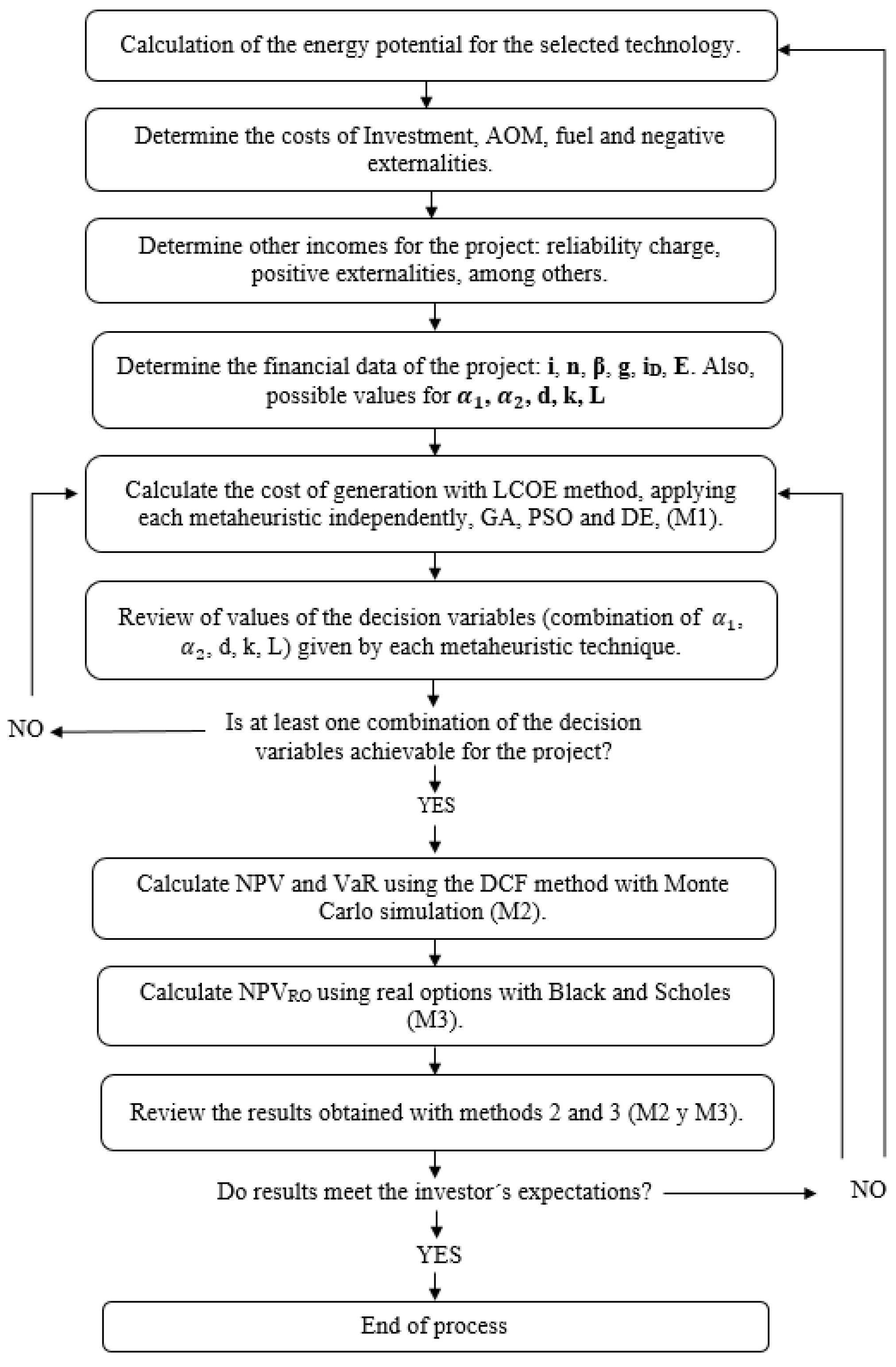
2.9. Summary of the Proposed Methodology

The methodology depicted in Figure 1 is detailed below:

• Step 1: Select the generation technology (FB, USW, PV, or WP) and calculate its energy potential.
• Step 2: Determine the initial investment costs, variable and fixed OM, fuels, negative externalities, and other costs necessary for the installation, commissioning, and operation of the project.
• Step 3: Determine other revenues that the project may have, other than those obtained from electricity production, such as, for example, the reliability charge and positive externalities.
• Step 4: Determine the financial data for the project: discount rate, tax rate, inflation rate, interest rate, term and grace period for the debt, and operating life of the project (in years).
• Step 5: Enter project costs, revenues, and financial data for each metaheuristic technique, GA, PSO, and DE, which are part of M1.
• Step 6: Check if the combinations of project decision variables obtained with M1 are achievable for the investor: (1) equity percentage, (2) debt percentage, (3) depreciation years, (4) grace period, and (5) debt term. In case none of them are achievable, go back to item 5 to run again each metaheuristic technique and review the new combinations.
• Step 6: Evaluate combinations of decision variables and GCs of technologies in M2 and M3.
• Step 7: Review the expected NPV and NPVRO, obtained with M2 and M3, respectively, as well as the VaR obtained with M2. If the results are not as desired, return to item 5 to run each metaheuristic technique again and review the new combinations; otherwise, select the combination of decision variables that is most appropriate for the project and achievable for the investor (end of the methodology).
• Step 8: Revise the technical and financial information of the project or increase the GC of the technology to a value that allows obtaining better results with M2 and M3. This is in case no acceptable combinations of decision variables are obtained for the investor, after n simulations with M1.

3. Tests and Results

Table 3. GC with and without tax incentives for different technologies.

Technology	GC without Incentives (¢USD/kWh)	GC with Incentives (¢USD/kWh)	Reduction (%)
FB	9.3	9	3.7
USW	13.9	13	6.6
PV	6.3	5.8	8.6
WP	11.4	10.4	8.7

shows the GC for FB, USW, PV, and WP technologies, calculated with M1 with and without tax incentives. These results correspond to the two base cases, previously defined, which serve as a reference to determine the effect of the methodology on the GC with tax incentives. Thus, GC of 9.3 USD/kWh, 13.9 USD/kWh, 6.3 USD/kWh and 11.4 USD/kWh were obtained for FB, USW, PV, and WP technologies, respectively, without tax incentives. However, when considering tax incentives, GC are reduced to 9 USD/kWh, 13 USD/kWh, 5.8 USD/kWh and 10.4 USD/kWh, with a decrease of $3.7\%$, $6.6\%$, $8.6\%$, and $8.7\%$, respectively. Therefore, the greatest reduction corresponds to the WP technology since it presents a higher percentage of pre-tax profit (taxable base), which allows it to take advantage of the ITC in greater proportion. It should be noted that according to the results obtained with M1, the reductions may be greater when considering indebtedness. This is because the payment of interest, with grace period and depreciation of assets, may reduce the impact of the tax rate during the operating life of the project.

According to the results presented in Table 3, the percentages of GC reduction do not exceed $10\%$, so the tax incentives, mainly the ITC, are not being fully exploited. Thus, a scenario of indebtedness with tax incentives favors the reduction of GC since the incentives can be taken advantage of in greater proportion and the effective tax rate can be reduced during the operating life of the projects. With the proposed approach, the investor is able to obtain an optimal combination of the values of the decision variables, one for each metaheuristic technique, which will result in different portfolios for the capital structure of the project.

Table 4. GC obtained by M1 with GA, PSO, and DE.

Tec.	M1 with GA			M1 with PSO			M1 with DE
	Combination ${\mathit{\alpha }}_1$, ${\mathit{\alpha }}_2$, d, k, L	GC (¢USD/kWh)	Red. (%)	Combination ${\mathit{\alpha }}_1$, ${\mathit{\alpha }}_2$, d, k, L	GC (¢USD/kWh)	Red. (%)	Combination ${\mathit{\alpha }}_1$, ${\mathit{\alpha }}_2$, d, k, L	GC (¢USD/kWh)	Red. (%)
FB	(2,8,10,10,10)	7.3	21.5	(1,9,8,10,9)	7.1	23.7	(1,9,9,10,8)	7.2	22.6
USW	(1,9,7,9,7)	8.5	38.8	(1,9,6,7,9)	8.8	36.7	(2,8,7,9,8)	8.9	36
PV	(2,8,3,10,5)	3.6	42.9	(2,8,9,10,8)	3.2	49.2	(1,9,8,10,2)	3.3	47.6
WP	(2,8,9,9,8)	5.9	48.2	(1,9,6,8,8)	5.8	49.1	(2,8,3,10,8)	6.0	47.4

shows the combination of values of the decision variables and the respective GC, using M1 and the metaheuristic techniques which parameters are presented in

Table 5. Parameters of the implemented metaheuristics.

Parameters	GA	PSO	ED
Maximum number of iterations	200	200	200
Population size	100	100	100
Crossover rate	0.7	-	-
Mutation rate	0.3	-	-
Inertia weight	-	1	-
Inertia Weight Damping Ratio	-	0.99	-
Individual Learning Coefficient	-	1.5	-
Global learning coefficient	-	2	-

. It should be clarified that M1 was implemented in each technique independently. For this reason, it is possible to have three different combinations of decision variables since the techniques do not present the same convergence; for each combination, a minimum GC is obtained considering the fiscal incentives.

Regarding the results presented in Table 4, it is observed that although the quality of the objective function (minimization of GC) is similar, the metaheuristic techniques do not converge to the same solution. Therefore, there are different GCs for FB, USW, PV, and WP technologies with percentage reductions that vary from $21.5\%$ to $49.2\%$, with respect to the base GC, which does not include tax incentives. According to Table 3, the above becomes an advantage for investors, who can select the combination of decision variables that best suits their capital structure or that best suits them to obtain a GC competitive against conventional generation sources. Additionally, comparing the results of Table 3 and Table 4, the reduction of GC requires indebtedness in projects, with adequate interest rates and grace periods, as well as a depreciation rate lower than the maximum allowed in the application of tax incentives ($33.33\%$ per year). This is because under these investment scenarios, the cash flows present a better performance in the decrease of the effective tax rate of the project and the increase in the use of tax incentives. Thus, the best combination to reduce GC (0.071 USD/kWh) of the FB is 1-9-8-10-9, which represents an equity percentage of $10\%$, a debt percentage of $90\%$, an asset depreciation of 8 years, a grace period of 10 years and a debt term of 9 years; the reduction percentage is $23.7\%$. Next, the best combination to reduce the GC (0.085 USD/kWh) of USW is 1-9-7-9-7, which represents an equity of $10\%$, a debt percentage of $90\%$, an asset depreciation of 7 years, a grace period of 9 years, and a debt term of 7 years. In this case, the percentage of reduction is $38.8\%$. The best combination to reduce the GC (0.032 USD/kWh) of PV is 2-8-9-10-8, which represents an equity of $20\%$, a debt percentage of $80\%$, an asset amortization of 9 years, a grace period of 10 years, and a debt term of 8 years; the reduction percentage is $49.2\%$. Finally, the best combination to reduce the GC (0.058 USD/kWh) of WP is 1-9-6-8-8, which represents an equity of $10\%$, a debt of $90\%$, an asset amortization of 6 years, a grace period of 8 years and a debt term of 8 years. In this case, the reduction is $49.1\%$. In summary, it is corroborated that the highest percentage of GC reduction is presented for technologies with the highest percentage of pre-tax profit, namely PV and WP.

Figure 2, Figure 3, Figure 4 and Figure 5 present the probability distributions of the NPV for each generation technology using M2. It should be clarified that the GC obtained by each metaheuristic technique, according to Table 4, was evaluated with M2; therefore, each technology presents three probability distributions for the NPV, corresponding to GA, PSO, and DE. On the other hand, 1000 simulations were contemplated for each case of M2, varying the historical data of the dollar exchange rate for Colombia, from 1 January 2017 to 31 December 2021 [37]; the confidence level of the simulations was $95\%$.

According to Figure 2, Figure 3, Figure 4 and Figure 5, the FB, USW, PV, and WP technologies present a risk of economic losses for the GCs calculated using M1; therefore, in spite of reaching an NPV equal to zero deterministically with M1, there is a possibility of obtaining an NPV lower than zero with M2 given the uncertainty introduced with the variation of the market representative rate, according to the historical data taken as a reference. In this way, the variation of the RMR represents an increase or decrease of the initial investment for the technologies, causing the project to require a variation of its income to compensate for such a situation and thus guarantee the opportunity cost of the investors. The variation of the income can be achieved through an increase or reduction of the GC obtained through M1. However, Figure 2, Figure 3, Figure 4 and Figure 5 show an NPV that takes positive values, causing the expected NPV to be greater than zero in some technologies, and a maximum NPV that ranges between 0.82 MUSD and 27.7 MUSD, according to Table 4. This means that the investor can have a higher opportunity cost, a higher profitability for the project, and greater flexibility and competitiveness in the electricity market.

Table 6. Discounted cash flow results, Monte Carlo simulation and VaR.

Tec.	Estimated NPV (MUSD)			Maximum NPV (MUSD)						NPV-Var (MUSD)
	GA	PSO	DE	GA	PSO	DE	P (%) GA	P (%) PSO	P (%) DE	GA	PSO	DE
FB	0.5	−0.4	0.7	4.2	3	4.4	0.9	0.3	0.4	3.8	4	3
USW	−0.5	−0.2	−0.9	25.3	27	27.7	0.8	0.2	0.5	29.4	30.6	30.8
PV	0.1	0.5	0.016	0.9	1.2	0.82	0.4	0.3	0.7	0.8	0.26	0.85
WP	0.09	0.5	−0.013	1.5	1.6	1.4	0.9	0.5	0.6	1.8	1.6	1.8

shows the results obtained through M2.

The best combination of decision variables that guarantees the technical and financial viability of FB with a higher degree of certainty is the combination reached using DE that is 1-9-9-10-8. This implies a GC of 0.072 USD/kWh, an expected NPV of 0.7 MUSD and a maximum NPV of 4.4 MUSD. For the USW, the expected NPV, obtained by each metaheuristic technique is lower than zero; for this reason, none of the three alternatives would be attractive to the investor, unless he considers the results obtained with M3 to determine the effect of the real option implied, in this case, the dollar exchange rate volatility on the traditional NPV (the one obtained with M2). For PV, the investor may choose the combination reached by PSO, which is 2-8-9-10-8, obtaining a GC of 0.03.2 USD/kWh, an expected NPV of 0.5 MUSD and a maximum NPV of 1.2 MUSD.

For WP, the combination obtained by the PSO technique: 1-9-6-8-8 can be chosen, obtaining a GC of 0.058 USD/kWh, an expected NPV of 0.5 MUSD and a maximum NPV of 1.6 MUSD. It should be emphasized that with M1, a GC is obtained that deterministically guarantees a NPV equal to zero and a minimum acceptable rate of return (MARR) for the investor. However, when uncertainty is introduced to the generation project through M2, it is possible to obtain an expected NPV greater than zero, giving the investor the possibility that the investment will generate a profitability greater than the MARR or that the GC can be reduced to a price that makes it competitive, if necessary.

Complementing the previous analysis, it is important for the investor to know the VaR of FB, USW, PV, and WP technologies in order to reduce the risk of losses in a generation project. Thus, the combination obtained with DE, for FB, presents a VaR of 3 MUSD, being this the lowest VaR value obtained with the metaheuristic techniques (GA: 3.8 MUSD and PSO: 4 MUSD). Therefore, it could be corroborated that the best investment structure for FB is the combination of DE (1-9-9-10-8), since a GC of 0.072 USD/kWh, an expected NPV of 0.7 MUSD and a maximum NPV of 4.4 MUSD are obtained. For the USW, the results obtained with M2 would not be attractive for an investor and, even more, when the VaR can oscillate between 29.4 MUSD and 30.8 MUSD, according to the results obtained with the GA, PSO and DE; therefore, the results obtained with M3 can guide the investor to choose the option with higher profitability and lower risk. It should be clarified that, if the investor wants to improve the results with M2, he can increase the value of the GC, obtained through M1, to the point where it improves the viability of the technology, guaranteeing its competitiveness compared to other generation technologies. For the PV, the combination given by the PSO (2-8-9-10-8) presents the lowest VaR, 0.26 MUSD; thus, it is corroborated that this combination represents the best alternative, since a GC of 0.058 USD/kWh, an expected NPV of 0.5 MUSD, and a maximum NPV of 1.6 MUSD are obtained. Finally, for PV, the combination given by PSO (1-9-6-8-8) presents the lowest VaR, 1.6 MUSD; thus, it is corroborated that this combination represents the best alternative since a GC of 0.058 USD/kWh, an expected NPV of 0.5 MUSD and a maximum NPV of 1.6 MUSD are obtained. Note that these VaR values represent the economic losses that the generation technologies may have with a $5\%$ probability of occurrence.

Through M1, FB, USW, PV, and WP technologies present a deterministic NPV equal to zero from a static RMR (fixed reference value that does not vary); however, by introducing uncertainty in M2 with the variation of the RMR, which is modeled by the distribution of historical RMR data for Colombia (from 1 January 2017 to 31 December 2021), this can take higher and lower values than the static RMR of M1, causing the investment cost of the technologies to present an increase or decrease. Therefore, when performing the 1000 Monte Carlo simulations, the technologies with higher investment cost may present a higher sensitivity to the RMR, as happened for the USW, in which the expected NPV associated to each metaheuristic technique is lower than zero.

Table 7. Results RO.

Technology	GA		PSO		DE
	NPV${}_{\mathit{RO}}$ (MUSD)	IV (%)	NPV${}_{\mathit{RO}}$ (MUSD)	IV (%)	NPV${}_{\mathit{RO}}$ (MUSD)	IV (%)
FB	0.43	9.1	0.39	18.8	0.35	16.5
USW	1.7	10.9	1.1	6.6	1.7	3.9
PV	0.04	2.6	0.035	0.06	0.02	3.6
WP	0.09	3.8	0.08	8.1	0.14	7.5

shows the NPV${}_{OR}$ obtained with M3 for the FB, USW, PV, and WP technologies. The implied volatility (IV in %) used for the Black and Scholes evaluation, was calculated from the annual variation of the net profit of each technology, during its operating life; for the above, the cash flows obtained with M1 were taken as a reference, where each technology has a cash flow associated with the results of each metaheuristic technique.

According to the results presented in Table 7, the generation technologies present an NPV${}_{OR}$ higher than zero for all combinations of decision variables, obtained from the GA, PSO, and DE techniques. The most relevant fact is that the USW technology presents an NPV${}_{OR}$ between 1.1 and 1.7 MUSD, due to the value acquired by the real option that implies the volatility of the cash flows. This leads the investor to accept the feasibility of the project, leaning toward the combination of the DE 2-8-7-9-8, which presents an NPV${}_{OR}$ of 1.7 MUSD, or the combination of the GA 1-9-7-9-7, which presents an NPV${}_{OR}$ of 1.7 MUSD. However, according to the results obtained with M2, the combination of the PSO 1-9-6-7-9 may be more interesting for the investor since the expected NPV${}_{OR}$ obtained with M2, −0.2 MUSD, is lower than that obtained with the GA and DE, −0.5 MUSD and −0.9 MUSD, respectively.

On the other hand, M3 has the advantage of providing a higher valuation to a technology when implicit ORs are considered, which are typical due to the heterogeneity presented by the cash flows of a project. Thus, from Equation (15) and considering that with M1 an NPV equal to zero is obtained, it is deduced that the NPV${}_{OR}$ reported in Table 7 correspond to the values of the real implicit option. This implies that the volatility presented in the cash flows gives an added value to the financial feasibility of the project, as occurs in the case of the USW technology. Finally, the M3 method has a greater impact on technologies with a higher initial investment.

Table 8. Consolidated results M1-M2-M3.

Technology	M1-GG (¢USD/kWh)			M2-NPV (MUSD)			M3-NPV${}_{\mathbf{RO}}$ (MUSD)
	GA	PSO	DE	GA	PSO	DE	GA	PSO	DE
FB	7.3	7.1	7.2	0.5	−0.4	0.7	0.43	0.39	0.35
USW	8.5	8.8	8.9	−0.5	−0.2	−0.9	1.7	1.1	1.7
PV	3.6	3.2	3.3	0.1	0.5	0.016	0.04	0.035	0.02
WP	5.9	5.8	6.0	-0.09	0.5	−0.013	0.09	0.08	0.14

shows the consolidated results obtained with M1, M2, and M3, considering tax incentives. The uncertainty in the RMR, used in M2, and the volatility in cash flows, used in M3, may cause a variation in the NPV expected by the investor and a difference with the result obtained with M1 (deterministic NPV equal to zero, calculated with a fixed RMR). This may result in an incomplete exercise for the investor since the RMR may undergo constant variations from the pre-feasibility studies stage to the equipment acquisition stage. Therefore, using only M1 is not sufficient to assess the risk of uncertainty of any technical and financial variable, as well as to determine the real NPV of the project. Therefore, M2 and M3 are complementary to help in investment decision making, generating greater confidence in the investor, who can make a risk management with VaR. The differences that can be presented between M2 and M3 is that the first one has a more robust structure, since it runs 1000 times a DCF from random values of RMR, which can be presented in the project according to its probability distribution; it also indicates how viable the implementation is of a generation technology when there is a variable RMR from a constant GC, obtained with M1. While M3 with Black and Scholes considers a constant implied volatility (calculated by means of M1 cash flows) evaluated in a single cash flow with present value (S) and initial investment (K).

Finally, comparing the GC of the technologies FB 0.071 to 0.073 USD/kWh, USW 0.085 to 0.089 USD/kWh, PV 0.032 to 0.036 USD/kWh, and WP 0.058 to 0.06 USD/kWh, with those reported by other authors FB 0.076 USD/kWh [19], USW 0.13 USD/kWh [49], PV 0.057 USD/kWh [50] and WP 0.05 USD/kWh to 0.12 USD/kWh [51], it is evident that competitive GC can be obtained in Colombia, starting from a combination of decision variables (${\alpha }_1,{\alpha }_2,d,k,L$) that minimizes the GC.

4. Recommendations

For the methodology proposed in this work to have a greater impact on the viability and development of projects with NCES in the electricity market, the following modifications and implementations of fiscal and economic incentives are proposed:

4.1. Investment Tax Incentives

This work corroborates that small and medium-sized companies, including new ones, are not able to take full advantage of investment tax incentives, specifically the benefit of recovering $50\%$ of the investment through income tax during the first 15 years of the project’s operation. For this reason, it is necessary to extend this benefit for the entire operating life of the project in order to recover $50\%$ of the investment [1,19,30].

4.2. Economic Incentives

Green credits: The application of a low interest rate from the banking sector or financial companies should be promoted for NCES projects. In [1], it is corroborated that the GC of NCES can be reduced up to $44\%$, when there is a scenario of $100\%$ debt, with a grace period of 5 years, a term of 10 years, and an interest rate of $6\%$ A.E., as well as a depreciation of assets at 10 years.

Project Finance: It is important that the financing is applied to the project and not to the investor; this in order to guarantee a longer term debt with a lower interest rate. Therefore, in this work, it is corroborated that, combining the grace period and the term of the debt, the project can pay the last installment of the loan in its last year of operation, allowing it to take advantage of the ITC in greater proportion during the first 15 years of operation and reduce the impact of the tax rate for each fiscal year.

Green bonds: Public and private sectors may support the financing of NCES projects through green bonds. In the report by [21], the application of different sources of capital, including green bonds, evidenced GC reductions of up to $24\%$.

Positive externality: The electricity market or government entities may subsidize NCES projects to ensure financial viability during their useful life. In the case of biomass from MSW, municipalities may pay a higher value for disposal due to the positive environmental impact caused. The value per disposal was reported in this work for MSW technology and has been addressed by other authors, such as [20,21,22].

Allocation of firm energy: Mechanisms to allocate firm energy for the reliability charge must be created or maintained to leverage projects with NCES. The above is corroborated in [21], where the application of the reliability charge, for an MSW power generation project allows the reduction of the GC by $59.5\%$.

5. Conclusions

This paper proposed a methodology for the optimal structuring of investments in NCRES in order to minimize the GC of four generation technologies, namely, FB, USW, PV, and WP, based on the use of fiscal and economic incentives. For this purpose, the LCOE method combined independently with three metaheuristic techniques, GA, PSO, and DE, was used; from each technique, a combination of decision variables (${\alpha }_1,{\alpha }_2,d,k,L$) and a GC were deterministically obtained, representing the investment portfolios and economic indicators (USD/kWh) for the generation technologies, respectively. Then, the methods of DCF with Monte Carlo simulation and VaR were used, as well as OR with Black and Scholes to obtain three complementary economic indicators, NPV, VaR, and NPV${}_{RO}$, considering the uncertainty in the RMR.

As an innovative feature, this paper provides a methodology for minimizing GC in the NCRES projects that combines five different financial decision variables and employs three metaheuristic approaches to provide investors with a set of solutions from which to choose. Furthermore, the proposed approach considers risk assessment methods and proposes fiscal and economic incentives to make NCRES electricity generation projects viable.

When evaluating the methodology proposed in this work, the following results were obtained: GC of 0.072 USD/kWh, NPV of 0.7 MUSD and NPV${}_{RO}$ of 0.35 MUSD for FB, using DE; GC of 0.088 USD/kWh, NPV of −0.2 MUSD and NPV${}_{RO}$ of 1.1 MUSD for USW, using PSO; GC of 0.032 USD/kWh, NPV of 0.5 MUSD and NPV${}_{RO}$ of 0.035 MUSD for SP, using PSO; GC of 0.058 USD/kWh, NPV of 0.5 MUSD and NPV${}_{RO}$ of 0.08 MUSD for WP, using PSO. The reductions in GC were $22.6\%$, $36.7\%$, $49.2\%$, and $49.1\%$, respectively, with the greatest reduction in the technologies with the highest pre-tax profit percentage, PV and WP. On the other hand, the metaheuristic techniques presented the same convergence speed; however, PSO showed better results with the combinations of the decision variables. Although the methodology proposed in this paper was developed in the Colombian context, it can be adapted and applied in other countries with different policies and fiscal incentives for the development of NCRES projects.

References

1. Saldarriaga-Loaiza, J.D.; López-Lezama, J.M.; Villada-Duque, F. Methodologies for structuring investments in renewable energy projects. Inf. Tecnol. 2022, 33, 189–202. [Google Scholar] [CrossRef]
2. López, A.R.; Krumm, A.; Schattenhofer, L.; Burandt, T.; Montoya, F.C.; Oberländer, N.; Oei, P.Y. Solar PV generation in Colombia—A qualitative and quantitative approach to analyze the potential of solar energy market. Renew. Energy 2020, 148, 1266–1279. [Google Scholar] [CrossRef]
3. Robles-Algarín, C.A.; Taborda-Giraldo, J.A.; Ospino-Castro, A.J. Procedimiento para la Selección de Criterios en la Planificación Energética de Zonas Rurales Colombianas. Inf. Tecnol. 2018, 29, 71–80. [Google Scholar] [CrossRef] [Green Version]
4. He, L.; Liu, R.; Zhong, Z.; Wang, D.; Xia, Y. Can green financial development promote renewable energy investment efficiency? A consideration of bank credit. Renew. Energy 2019, 143, 974–984. [Google Scholar] [CrossRef]
5. Liu, Y.; Zheng, R.; Chen, S.; Yuan, J. The economy of wind-integrated-energy-storage projects in China’s upcoming power market: A real options approach. Resour. Policy 2019, 63, 101434. [Google Scholar] [CrossRef]
6. Yang, X.; He, L.; Zhong, Z.; Wang, D. How does China’s green institutional environment affect renewable energy investments? The nonlinear perspective. Sci. Total. Environ. 2020, 727, 138689. [Google Scholar] [CrossRef]
7. Wu, Y.; Wang, J.; Ji, S.; Song, Z. Renewable energy investment risk assessment for nations along China’s Belt & Road Initiative: An ANP-cloud model method. Energy 2019, 190, 116381. [Google Scholar] [CrossRef]
8. Ziyaei, P.; Khorasanchi, M.; Sayyaadi, H.; Sadollah, A. Minimizing the levelized cost of energy in an offshore wind farm with non-homogeneous turbines through layout optimization. Ocean. Eng. 2019, 249, 110859. [Google Scholar] [CrossRef]
9. Petrovic, A.; Durisic, Z. Genetic algorithm based optimized model for the selection of wind turbine for any site-specific wind conditions. Energy 2022, 236, 121476. [Google Scholar] [CrossRef]
10. El Hamdani, F.; Vaudreuil, S.; Abderafi, S.; Bounahmidi, T. Determination of design parameters to minimize LCOE, for a 1 MWe CSP plant in different sites. Renew. Energy 2022, 169, 1013–1025. [Google Scholar] [CrossRef]
11. Singh, P.; Pandit, M.; Srivastava, L. Optimization of Levelized Cost of Hybrid Wind-Solar-Diesel-Battery System Using Political Optimizer. In Proceedings of the 2020 IEEE First International Conference on Smart Technologies for Power, Energy and Control (STPEC), Nagpur, India, 25–26 September 2020; pp. 1–6. [Google Scholar] [CrossRef]
12. Seulki, H.; Kim, J. A multi-period MILP model for the investment and design planning of a national-level complex renewable energy supply system. Renew. Energy 2021, 141, 736–750. [Google Scholar]
13. Qadir, S.A.; Al-Motairi, H.; Tahir, F.; Al-Fagih, L. Incentives and strategies for financing the renewable energy transition: A review. Energy Rep. 2021, 7, 3590–3606. [Google Scholar] [CrossRef]
14. Radpour, S.; Gemechu, E.; Ahiduzzaman, M.; Kumar, A. Developing a framework to assess the long-term adoption of renewable energy technologies in the electric power sector: The effects of carbon price and economic incentives. Renew. Sustain. Energy Rev. 2021, 152, 111663. [Google Scholar] [CrossRef]
15. Veríssimo, P.H.A.; Campos, R.A.; Guarnieri, M.V.; Veríssimo, J.P.A.; do Nascimento, L.R.; Rüther, R. Area and LCOE considerations in utility-scale, single-axis tracking PV power plant topology optimization. Sol. Energy 2020, 211, 433–445. [Google Scholar] [CrossRef]
16. Arias-Cazco, D.; Gavela, P.; Panchi, L.C.; Izquierdo, P. Sensitivity Analysis for Levelized Cost of Electricity—LCOE with Multi-objective Optimization. IEEE Lat. Am. Trans. 2020, 20, 2071–2078. [Google Scholar] [CrossRef]
17. Martín Barroso, A.M.; Leyva Ferreiro, G. Análisis crítico de la inversión en energías renovables. Enfoque socioeconómico. Cofin Habana 2017, 11, 69–90. [Google Scholar]
18. Villada Duque, F.; López Lezama, J.M.; Muñoz Galeano, N. Effects of Incentives for Renewable Energy in Colombia. Ing. Univ. 2017, 21, 257–272. [Google Scholar] [CrossRef] [Green Version]
19. Saldarriaga-Loaiza, J.D.; Villada, F.; Pérez, J.F. Análisis de Costos Nivelados de Electricidad de Plantas de Cogeneración usando Biomasa Forestal en el Departamento de Antioquia, Colombia. Inf. Tecnol. 2019, 30, 63–74. [Google Scholar] [CrossRef] [Green Version]
20. Montiel-Bohórquez, N.D.; Saldarriaga-Loaiza, J.D.; Pérez, J.F. A Techno-Economic Assessment of Syngas Production by Plasma Gasification of Municipal Solid Waste as a Substitute Gaseous Fuel. J. Energy Resour. Technol. 2021, 143, 90901. [Google Scholar] [CrossRef]
21. Montiel-Bohórquez, N.D.; Saldarriaga-Loaiza, J.D.; Pérez, J.F. Analysis of investment incentives for power generation based on an integrated plasma gasification combined cycle power plant using municipal solid waste. Case Stud. Therm. Eng. 2021, 30, 101748. [Google Scholar] [CrossRef]
22. Montiel-Bohórquez, N.D.; Saldarriaga-Loaiza, J.D.; Pérez, J.F. Effect of the Colombian Renewable Energy Law on the Levelized Cost of a Substitute Gaseous Fuel Produced from MSW Gasification. Ing. Investig. 2021, 42, e92410. [Google Scholar] [CrossRef]
23. Castillo-Ramírez, A.; Mejía-Giraldo, D.; Molina-Castro, J.D. Fiscal incentives impact for RETs investments in Colombia. Energy Sources Part B Econ. Plan. Policy 2017, 12, 759–764. [Google Scholar] [CrossRef]
24. Gómez, L.M.J.; Prins, N.M.A.; López, M.D.R. Valoración de opción real en proyectos de generación de energía eólica en Colombia. Rev. Espac. 2016, 37, 26. [Google Scholar]
25. Restrepo-Garcés, A.R.; Manotas-Duque, D.F.; Lozano, C.A. Multicriteria Hybrid Method—ROA, for the choice of generation of renewable sources: Case study in shopping centers. Ingeniare Rev. Chil. Ing. 2017, 25, 399–414. [Google Scholar] [CrossRef] [Green Version]
26. Bueno López, M.; Rodríguez Sarmiento, L.C.; Rodríguez Sánchez, P.J. Análisis de costos de la generación de energía eléctrica mediante fuentes renovables en el sistema eléctrico colombiano. Ing. Desarro. 2016, 34, 397–419. [Google Scholar] [CrossRef]
27. Arango, M.A.A. Modelo de proyectos de evaluación de riesgo en generación de energía térmica. Rev. Espac. 2016, 37, 26. [Google Scholar]
28. Rodas, Y.; Arango, M.A. Optimización de la estructura de costos para la generación de energía hidroeléctrica: Una aplicación del Modelo Black Litterman. Rev. Espac. 2016, 38, 26. [Google Scholar]
29. Sánchez, M.; Moncada, C.A.L.; Duque, D.F.M. Modelo de valoración de riesgo financiero en la gestión de contratos de suministro de energía eléctrica. Tecnura Tecnol. Cult. Afirmando Conoc. 2014, 18, 110–127. [Google Scholar] [CrossRef] [Green Version]
30. Saldarriaga-Loaiza, J.D.; López-Lezama, J.M.; Villada-Duque, F. Levelized Cost of Electricity in Colombia under New Fiscal Incentives. Int. J. Eng. Res. Technol. 2020, 13, 3234–3239. [Google Scholar] [CrossRef]
31. Castillo-Ramírez, A.; Mejía-Giraldo, D.; Muñoz-Galeano, N. Large-Scale Solar PV LCOE Comprehensive Breakdown Methodology. CT&F Cienc. Tecnol. Futuro 2015, 7, 117–126. [Google Scholar]
32. Castillo-Ramírez, A.; Mejía-Giraldo, D.; Giraldo-Ocampo, J.D. Geospatial levelized cost of energy in Colombia: GeoLCOE. In Proceedings of the Innovative Smart Grid Technologies Latin America (ISGT LATAM), Montevideo, Uruguay, 5–7 October 2015; pp. 298–303. [Google Scholar] [CrossRef]
33. Tasas de Interés y Sector Financiero. Available online: https://totoro.banrep.gov.co/analytics/saw.dll?Portal (accessed on 6 October 2022).
34. Inflación Total y Meta. Available online: https://www.banrep.gov.co/es/estadisticas/inflacion-total-y-meta/ (accessed on 6 October 2022).
35. Hasan, M.; Zhang, M.; Wu, W.; Langrish, T.A. Discounted cash flow analysis of greenhouse-type solar kilns. Renew. Energy 2016, 95, 404–412. [Google Scholar] [CrossRef]
36. Franco-Sepulveda, G.; Campuzano, C.; Pineda, C. NPV risk simulation of an open pit gold mine project under the O’Hara cost model by using GAs. Int. J. Min. Sci. Technol. 2017, 27, 557–565. [Google Scholar] [CrossRef]
37. Datos históRicos USD/COP. Available online: https://es.investing.com/currencies/usd-cop-historical-data (accessed on 6 October 2022).
38. Cheung, K.; Yuen, F. On the uncertainty of VaR of individual risk. J. Comput. Appl. Math. 2020, 367, 112468. [Google Scholar] [CrossRef]
39. Balibrea-Iniesta, J.; Rodríguez-Monroy, C.; Núñez-Guerrero, Y.M. Economic analysis of the German regulation for electrical generation projects from biogas applying the theory of real options. Energy 2021, 231, 120976. [Google Scholar] [CrossRef]
40. Chowdhury, R.; Mahdy, M.; Alam, a.N.; Al Quaderi, G.D.; Rahman, M.A. Predicting the stock price of frontier markets using machine learning and modified Black–Scholes Option pricing model. Phys. A Stat. Mech. Appl. 2022, 555, 124444. [Google Scholar] [CrossRef] [Green Version]
41. Rentabilidad del Bono Estados Unidos 10 añOs. Available online: https://es.investing.com/rates-bonds/u.s.-10-year-bond-yield-historical-data (accessed on 6 October 2022).
42. Ramos-Figueroa, O.; Quiroz-Castellanos, M.; Mezura-Montes, E.; Schütze, O. Metaheuristics to solve grouping problems: A review and a case study. Swarm Evol. Comput. 2020, 53, 100643. [Google Scholar] [CrossRef]
43. Saldarriaga-Zuluaga, S.D.; López-Lezama, J.M.; Muñoz-Galeano, N. Optimal coordination of over-current relays in microgrids considering multiple characteristic curves. Alex. Eng. J. 2021, 60, 2093–2113. [Google Scholar] [CrossRef]
44. Jaramillo Serna, J.d.J.; López-Lezama, J.M. Alternative Methodology to Calculate the Directional Characteristic Settings of Directional Overcurrent Relays in Transmission and Distribution Networks. Energies 2019, 12, 3779. [Google Scholar] [CrossRef] [Green Version]
45. Agudelo, L.; López-Lezama, J.M.; Muñoz-Galeano, N. Vulnerability assessment of power systems to intentional attacks using a specialized genetic algorithm. Dyna 2015, 82, 78–84. [Google Scholar] [CrossRef]
46. Arrif, T.; Hassani, S.; Guermoui, M.; Sánchez-González, A.; Taylor, A.R.; Belaid, A. GA-GOA hybrid algorithm and comparative study of different metaheuristic population-based algorithms for solar tower heliostat field design. Renew. Energy 2022, 192, 745–758. [Google Scholar] [CrossRef]
47. Zeng, Z.; Zhang, M.; Zhang, H.; Hong, Z. Improved differential evolution algorithm based on the sawtooth-linear population size adaptive method. Inf. Sci. 2022, 608, 1045–1071. [Google Scholar] [CrossRef]
48. IPC Información téCnica. Available online: https://www.dane.gov.co/index.php/estadisticas-por-tema/precios-y-costos/indice-de-precios-al-consumidor-ipc/ipc-informacion-tecnica (accessed on 6 October 2022).
49. Hadidi, L.A.; Omer, M.M. A financial feasibility model of gasification and anaerobic digestion waste-to-energy (WTE) plants in Saudi Arabia. Waste Manag. 2017, 59, 90–101. [Google Scholar] [CrossRef] [PubMed]
50. Global Trends. Available online: https://www.irena.org/Statistics/View-Data-by-Topic/Costs/Global-Trends (accessed on 6 October 2022).
51. Bruck, M.; Sandborn, P.; Goudarzi, N. A Levelized Cost of Energy (LCOE) model for wind farms that include Power Purchase Agreements (PPAs). Renew. Energy 2018, 122, 131–139. [Google Scholar] [CrossRef]
Figure 1. Methodology for optimal structuring of NCES investments.
Sustainability 14 15123 g001
Figure 2. Probability distributions, NPV-FB.
Sustainability 14 15123 g002
Figure 3. Probability distributions, NPV-USW.
Sustainability 14 15123 g003
Figure 4. Probability distributions, NPV-PV.
Sustainability 14 15123 g004
Figure 5. Probability distributions, NPV-WP.
Sustainability 14 15123 g005