
Security Challenges and Economic-Geographical Metrics for Analyzing Safety to Achieve Sustainable Protection


Abstract
:1. Introduction
2. Literature Review
3. Preliminaries
4. Methods and Materials
4.1. Generalized Metrics
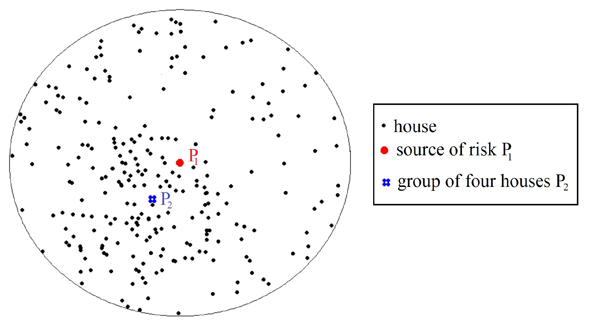
4.2. Generated Data
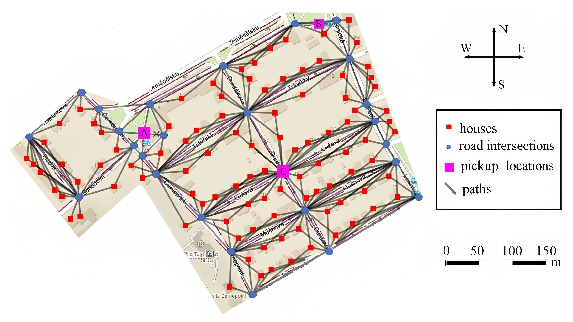
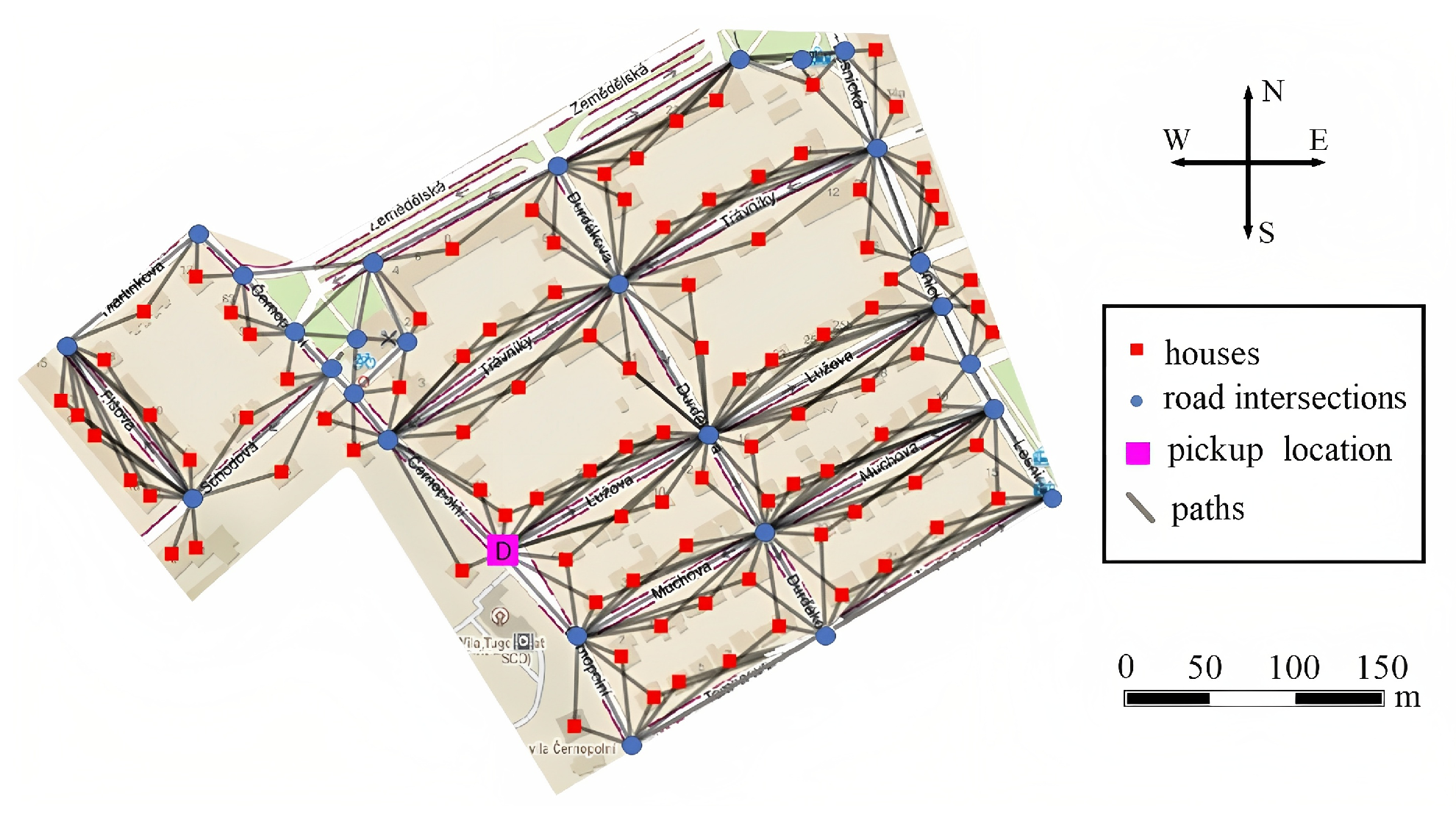
4.3. Map-Based Data
5. Results
5.1. Model Scenarios and Their Interpretations with Metrics on Generated Data
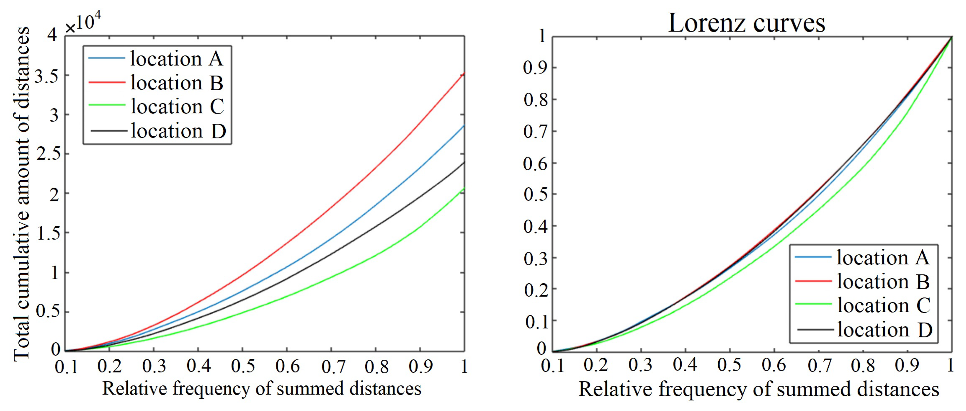
5.2. Model Scenario Based on the Actual World Map
6. Discussion
6.1. Findings and Their Implications
6.2. Limitations and Opportunities for Future Research
7. Conclusions
Author Contributions
Funding
Institutional Review Board Statement
Informed Consent Statement
Data Availability Statement
Acknowledgments
Conflicts of Interest
References
- United Nations. Universal Declaration of Human Rights, 1948, 217(III)A. Available online: https://www.un.org/en/about-us/universal-declaration-of-human-rights (accessed on 24 June 2022).
- Ugarte, M.P.; Achilleos, S.; Quattrocchi, A.; Gabel, J.; Kolokotroni, O.; Constantinou, C.; Nicolaou, N.; Rodriguez-Llanes, J.M.; Huang, Q.; Verstiuk, O.; et al. Premature mortality attributable to COVID-19: Potential years of life lost in 17 countries around the world, January–August 2020. BMC Public Health 2022, 22, 54. [Google Scholar] [CrossRef] [PubMed]
- Gosden, C.; Gardener, D. Weapons of mass destruction–threats and responses. BMJ Clin. Res. Ed. 2005, 331, 397–400. [Google Scholar] [CrossRef] [PubMed]
- Thayer, B.A. Considering population and war: A critical and neglected aspect of conflict studies. Philos. Trans. R. Soc. Biol. Sci. 2022, 364, 3081–3092. [Google Scholar] [CrossRef] [PubMed] [Green Version]
- Wither, J.K. Back to the future? Nordic total defence concepts. Def. Stud. 2020, 20, 61–81. [Google Scholar] [CrossRef]
- Ziauddin, S.B. Superpower underground: Switzerland’s rise to global bunker expertise in the atomic age. Technol. Cult. 2017, 58, 921–954. [Google Scholar] [CrossRef]
- Horák, R. Průvodce Krizovým Plánováním pro Veřejnou Správu: [Prevence Řešení Mimořádných Krizových Situací]; Linde: Praha, Czech Republic, 2011; ISBN 978-80-7201-827-7. [Google Scholar]
- Cai, Y.M.; Chatelet, D.S.; Howlin, R.P.; Wang, Z.-Z.; Webb, J.S. A novel application of Gini coefficient for the quantitative measurement of bacterial aggregation. Sci. Rep. 2019, 9, 1902. [Google Scholar] [CrossRef] [Green Version]
- Simone, A.; Cesaro, A.; Del Giudice, G.; Di Crosto, C.; Fecarotta, O. Potentialities of complex network theory tools for urban drainage networks analysis. Water Resour. Res. 2022, 58, e2022WR032277. [Google Scholar] [CrossRef]
- Su, H.; Chen, W.; Zhang, C. Evaluating the effectiveness of emergency shelters by applying an age-integrated method. GeoJournal 2022, 13, 1–19. [Google Scholar] [CrossRef]
- Su, H.; Chen, W.; Cheng, M. Using the variable two-step floating catchment area method to measure the potential spatial accessibility of urban emergency shelters. GeoJournal 2022, 87, 2625–2639. [Google Scholar] [CrossRef]
- Liu, W.; Xu, H.; Wu, J.; Li, W.; Hu, H. Measuring spatial accessibility to refuge green space after earthquakes: A case study of Nanjing, China. PLoS ONE 2022, 17, e0270035. [Google Scholar] [CrossRef]
- Zibulewsky, J. Defining disaster: The emergency department perspective. Bayl. Univ. Med. Cent. Proc. 2001, 14, 144–149. [Google Scholar] [CrossRef] [PubMed] [Green Version]
- Kakwani, N.C. Income Inequality and Poverty Methods of Estimation and Policy Applications; Oxford University Press: New York, NY, USA, 1980; ISBN 0-19-520227-9. [Google Scholar]
- Mussida, C.; Parisi, M.L. Immigrant groups’ income inequality within and across Italian regions. J. Econ. Inequal. 2018, 16, 655–671. [Google Scholar] [CrossRef]
- Eva, M.; Cehan, A.; Corodescu-Rosca, E.; Bourdin, S. Spatial patterns of regional inequalities: Empirical evidence from a large panel of countries. Appl. Geogr. 2022, 140, 102638. [Google Scholar] [CrossRef]
- Zhang, D.; Zhang, G.; Zhou, C. Differences in accessibility of public health facilities in hierarchical municipalities and the spatial pattern characteristics of their services in doumen district. Land 2021, 10, 1249. [Google Scholar] [CrossRef]
- Boisjoly, G.; Moreno-Monroy, A.I.; El-Geneidy, A. Informality and accessibility to jobs by public transit: Evidence from the São Paulo Metropolitan Region. J. Transp. Geogr. 2017, 64, 89–96. [Google Scholar] [CrossRef]
- Yamaguchi, K. Multigroup Segregation Analyses with Covariates. Sociol. Methodol. 2021, 51, 224–252. [Google Scholar] [CrossRef]
- Sánchez-Hechavarría, M.E.; Ghiya, S.; Carrazana-Escalona, R.; Cortina-Reyna, S.; Andreu-Heredia, A.; Acosta-Batista, C.; Saá-Muñoz, N.A. Introduction of application of Gini coefficient to heart rate variability spectrum for mental stress evaluation. Arq. Bras. Cardiol. 2019, 113, 725–732. [Google Scholar] [CrossRef]
- Chang, X.; Wu, Z.; Chen, Y.; Du, Y.; Shang, L.; Ge, Y.; Chang, J.; Yang, G. The booming number of museums and their inequality changes in China. Sustainability 2021, 13, 13860. [Google Scholar] [CrossRef]
- Wu, C.; Ye, X.; Du, Q.; Luo, P. Spatial effects of accessibility to parks on housing prices in Shenzhen, China. Habitat Int. 2017, 63, 45–54. [Google Scholar] [CrossRef]
- Wu, H.; Liu, L.; Yu, Y.; Peng, Z. Evaluation and planning of urban green space distribution based on mobile phone data and two-step floating catchment area method. Sustainability 2018, 10, 214. [Google Scholar] [CrossRef]
- Guida, C.; Carpentieri, G.; Masoumi, H. Measuring spatial accessibility to urban services for older adults: An application to healthcare facilities in Milan. Eur. Transp. Res. Rev. 2022, 14, 23. [Google Scholar] [CrossRef]
- Luo, J. Integrating the huff model and floating catchment area methods to analyze spatial access to healthcare services. Trans. GIS 2014, 18, 436–448. [Google Scholar] [CrossRef]
- Luo, W.; Whippo, T. Variable catchment sizes for the two-step floating catchment area (2SFCA) method. Health Place 2012, 18, 789–795. [Google Scholar] [CrossRef] [PubMed]
- Jamtscho, S.; Corner, R.; Dewan, A. Spatio-temporal analysis of spatial accessibility to primary health care in Bhutan. ISPRS Int. J. Geo-Inf. 2015, 4, 1584–1604. [Google Scholar] [CrossRef] [Green Version]
- Sharma, G.; Patil, G.R. Public transit accessibility approach to understand the equity for public healthcare services: A case study of Greater Mumbai. J. Transp. Geogr. 2021, 94, 103123. [Google Scholar] [CrossRef]
- Jiao, W.; Huang, W.; Fan, H. Evaluating spatial accessibility to healthcare services from the lens of emergency hospital visits based on floating car data. Int. J. Digit. Earth 2022, 15, 108–133. [Google Scholar] [CrossRef]
- Czech Republic. Act no. 374/2011 Sb. ze dne 6.Listopadu 2011 o Zdravotnické Záchranné Službě. Sbírka Zákonů České Republiky. 2011. částka 131. pp. 4839–4848. Available online: https://www.mvcr.cz/ (accessed on 24 June 2022).
- Young, C.S. Metrics and Methods for Security Risk Management; Elsevier, Inc.: Burlington, VT, USA, 2010; ISBN 978-1-85617-978-2. [Google Scholar]
- Liu, H.; Jia, Y.; Niu, C.; Gan, Y. Spatial pattern analysis of regional water use profile based on the Gini coefficient and location quotient. J. Am. Water Resour. Assoc. 2019, 55, 1349–1366. [Google Scholar] [CrossRef]
- Zhu, X.; Tong, Z.; Liu, X.; Li, X.; Lin, P.; Wang, T. An improved two-step floating catchment area method for evaluating spatial accessibility to urban emergency shelters. Sustainability 2018, 10, 2180. [Google Scholar] [CrossRef] [Green Version]
- Xia, Z.; Lu, H.; Chen, Y.; Yu, W. Integrating spatial and non-spatial dimensions to measure urban fire service access. ISPRS Int. J. Geo-Inf. 2019, 8, 138. [Google Scholar] [CrossRef] [Green Version]
- Dai, D. Black residential segregation, disparities in spatial access to health care facilities, and late-stage breast cancer diagnosis in metropolitan Detroit. Health Place 2010, 16, 1038–1052. [Google Scholar] [CrossRef]
- Radke, J.; Mu, L. Spatial decompositions, modeling and mapping service regions to predict access to social programs. Geogr. Inf. Sci. 2000, 6, 105–112. [Google Scholar]
- Siegel, M.; Koller, D.; Vogt, V.; Sundmacher, L. Developing a composite index of spatial accessibility acrossdifferent health care sectors: A German example. Health Policy 2016, 120, 205–212. [Google Scholar] [CrossRef] [PubMed]
- Krause, E.F. An Adventure in Non-Euclidian Geometry; Dover Publications, Inc.: New York, NY, USA, 1986; ISBN 0-486-25202-7. [Google Scholar]
- Mohr, P.J.; Phillips, W.D. Dimensionless Units in the SI. Metrologia 2015, 52, 40–47. [Google Scholar] [CrossRef]
- Knapp, A.W. Basic Algebra; Birkhäuser: New York, NY, USA, 2006; ISBN 978-0-8176-3248-9. [Google Scholar]
- Byrtusová, A. Use of the index methods of income inequality for assessing the security level. Econ. Manag. 2015, 9, 31–38. Available online: https://www.unob.cz/eam/Stranky/2015_2.aspx (accessed on 24 June 2022).
- Lorenz, M.O. An Outline of the Economic Theory of Railroad Rates; Nabu Press: Charleston, SC, USA, 2012; ISBN 1279878541. [Google Scholar]
- Ceriani, L.; Verme, P. The origins of the Gini index: Extracts from Variabilità e Mutabilità (1912) by Corrado Gini. J. Econ. Inequal. 2012, 10, 421–443. [Google Scholar] [CrossRef]
- Druckman, A.; Jackson, T. Measuring resource inequalities: The concepts and methodology for an area-based Gini coefficient. Ecol. Econ. 2008, 65, 242–252. [Google Scholar] [CrossRef] [Green Version]
- Duncan, O.D. The measurement of population distribution. Popul. Stud. 1957, 11, 27–45. [Google Scholar] [CrossRef]
- Alan, N.S.; Bardos, S.; Shelkova, N.Y. CEO-to-employee pay ratio and CEO diversity. Manag. Financ. 2020, 47, 356–382. [Google Scholar]
- La Haye, R.; Zizler, P. The Gini mean difference and variance. Metron 2019, 77, 43–52. [Google Scholar] [CrossRef]
- Kakwani, N. On a Class of Poverty Measures. Econometrica 1980, 48, 437–446. [Google Scholar] [CrossRef]
- R-Project. Available online: https://www.r-project.org/ (accessed on 13 September 2022).
- Mathworks. Available online: https://www.mathworks.com/products/matlab.html (accessed on 13 September 2022).
- Mapy.cz: © Seznam.cz, a.s. Available online: https://mapy.cz (accessed on 24 June 2022).
- Potůček, R. Life Cycle of the Crisis Situation Threat and Its Various Models, Qualitative and Quantitative Models in Socio-Economic Systems and Social Work. Studies in Systems, Decision and Control; Sarasola Sánchez-Serrano, J., Maturo, F., Hošková-Mayerová, Š., Eds.; Springer: Cham, Switzerland, 2020. [Google Scholar]
- Brno. Available online: https://en.brno.cz/ (accessed on 13 October 2022).
- Marling, G.; Horberry, T.; Harris, J. Development and reliability review of an assessment tool to measure competency in the seven elements of the risk management process: Part one-the riskometric. Safety 2021, 7, 1. [Google Scholar] [CrossRef]
- Oulehlová, A.; Kudlák, A.; Urban, R.; Hoke, E. Competitiveness of the Regions in the Czech Republic from the Perspective of Disaster Risk Financing. J. Compet. 2021, 13, 115–131. [Google Scholar] [CrossRef]
- Polcarová, E.; Pupíková, J. Building Community Resilience in the Czech Legislation. Lect. Notes Netw. Syst. 2022, 257, 131–144. [Google Scholar]
- Pei, X.; Guo, P.; Chen, Q.; Li, J.; Liu, Z.; Sun, Y.; Zhang, X. An Improved multi-mode two-step floating catchment area method for measuring accessibility of urban park in Tianjin, China. Sustainability 2022, 14, 11592. [Google Scholar] [CrossRef]
- Radosavljevic, V.; Belojevic, G.; Pavlovic, N. Tool for decision-making regarding general evacuation during a rapid river flood. Public Health 2017, 146, 134–139. [Google Scholar] [CrossRef]
- Yusoff, S.; Yusoff, N.H. Disaster Risks Management through Adaptive Actions from Human-Based Perspective: Case Study of 2014 Flood Disaster. Sustainability 2022, 14, 7405. [Google Scholar]
- Borowska-Stefańska, M.; Kowalski, M.; Turoboś, F.; Wiśniewski, S. Optimisation patterns for the process of a planned evacuation in the event of a flood. Environ. Hazards 2019, 18, 335–360. [Google Scholar]
- Tromp, E.; Te Nijenhuis, A.; Knoeff, H. The Dutch Flood Protection Programme: Taking Innovations to the Next Level. Water 2020, 14, 1460. [Google Scholar] [CrossRef]
- Kincl, P.; Oulehlová, A. Assessment Criteria for Municipality Territory Resilience to Anthropogenic Threats. Lect. Notes Netw. Syst. 2022, 257, 209–224. [Google Scholar]
- ArcGIS. Available online: https://www.arcgis.com/index.html (accessed on 13 October 2022).
- QGIS. Available online: https://www.qgis.org/en/site/ (accessed on 13 October 2022).
- Mukesh, M.S.; Katpatal, Y.B.; Londhe, D.S. Analyzing the impact of floods on vehicular mobility along urban road networks using the multiple centrality assessment approach. ASCE-ASME J. Risk Uncertain. Eng. Syst. Part A Civ. Eng. 2022, 8, 05022001. [Google Scholar]
- Chen, B.Y.; Cheng, X.-P.; Kwan, M.-P. Evaluating spatial accessibility to healthcare services under travel time uncertainty: A reliability-based floating catchment area approach. J. Transp. Geogr. 2020, 87, 102794. [Google Scholar] [CrossRef]
- Esposito Amideo, A.; Scaparra, M.P.; Kotiadis, K. Optimising shelter location and evacuation routing operations: The critical issues. Eur. J. Oper. Res. 2019, 279, 279–295. [Google Scholar] [CrossRef]
- Vališ, D.; Hasilová, K.; Forbelská, M.; Vintr, Z. Reliability modelling and analysis of water distribution network based on backpropagation recursive processes with real field data. Meas. J. Int. Meas. Confed. 2020, 149, 107026. [Google Scholar] [CrossRef]

| Sequence | T | |||
|---|---|---|---|---|
| 301.44 | 1.21 | 1.24 | 1.98 | |
| 288.33 | 1.15 | 1.01 | 2.53 |
| Sequence | G | H | |
|---|---|---|---|
| 0.241 | 1.6 | 0.18 | |
| 0.309 | 2.5 | 0.19 |
| Distances | ||||
|---|---|---|---|---|
| 0.241 | 0.371 | 0.455 | 0.513 | |
| 0.309 | 0.448 | 0.527 | 0.579 |
| Location | T | G | H | ||||
|---|---|---|---|---|---|---|---|
| Location A | 28,688 | 290 | 280 | 558 | 0.259 | 1.995 | 0.189 |
| Location B | 35,323 | 357 | 371 | 607 | 0.246 | 1.637 | 0.178 |
| Location C | 20,697 | 209 | 191 | 495 | 0.321 | 2.592 | 0.226 |
| Location | T | G | H | ||||
|---|---|---|---|---|---|---|---|
| Location D | 23,971 | 242 | 250 | 457 | 0.25 | 1.829 | 0.182 |
Publisher’s Note: MDPI stays neutral with regard to jurisdictional claims in published maps and institutional affiliations. |
© 2022 by the authors. Licensee MDPI, Basel, Switzerland. This article is an open access article distributed under the terms and conditions of the Creative Commons Attribution (CC BY) license (https://creativecommons.org/licenses/by/4.0/).
Share and Cite
Jekl, J.; Jánský, J. Security Challenges and Economic-Geographical Metrics for Analyzing Safety to Achieve Sustainable Protection. Sustainability 2022, 14, 15161. https://doi.org/10.3390/su142215161
Jekl J, Jánský J. Security Challenges and Economic-Geographical Metrics for Analyzing Safety to Achieve Sustainable Protection. Sustainability. 2022; 14(22):15161. https://doi.org/10.3390/su142215161
Chicago/Turabian StyleJekl, Jan, and Jiří Jánský. 2022. "Security Challenges and Economic-Geographical Metrics for Analyzing Safety to Achieve Sustainable Protection" Sustainability 14, no. 22: 15161. https://doi.org/10.3390/su142215161