Risk Management of Fuel Hedging Strategy Based on CVaR and Markov Switching GARCH in Airline Company

Abstract

Using a hedging strategy to stabilize fuel price is very important for airline companies in order to reduce the cost of their main business. In this paper, we construct models for managing the risk of the hedging strategy. First, we use conditional value at risk (CVaR) to measure the risk of an airline company’s hedging strategy. Compared with the value at risk (VaR), CVaR satisfies subadditivity, positive homogeneity, monotonicity, and transfer invariance. Therefore, CVaR is a consistent method of risk measurement. Second, time-varying state transition probability is introduced into our model in order to build a Markov Switching-GARCH (MS-GARCH). MS-GARCH takes dynamic changes of market state into account, a feature which has obvious advantages over the traditional constant state model. Additionally, we use a Markov chain Monte Carlo (MCMC) algorithm to estimate the parameters of MS-GARCH based on Gibbs sampling. We use fuel oil futures data from the Shanghai Futures Stock Exchange to implement and evaluate our model. In this paper, we empirically estimate the risk of airlines’ hedging strategy and draw the conclusion that our model is obviously effective in terms of the risk management of hedging, a use which has a certain guiding significance for reality.

1. Introduction

Enterprise risk management (ERM) is an indispensable part of the operation and management of companies. The profit of a company can be summarized as the income minus the cost, of which the core contents are the main business income and the main business costs. If an enterprise can successfully control the cost of its main business, then it can improve its production and operations efficiency and expand the scale of the company. For an airline company, however, the operating costs are mainly affected by changes of the international environment, such as steep fluctuations in the price of fuel oil commodities in international and domestic markets, ultimately meaning that the price of the fuel purchased by an airline company cannot be maintained within a reasonable range.

In recent decades, many large airlines in China have carried out hedging operations in the derivatives market, and some have even established futures Ltd. to be responsible for futures trading and clearing. However, in the process of using financial derivatives for hedging, due to some enterprises’ unclear understanding of risk management and the purpose of derivatives use, the original hedging strategy has turned into speculation, which almost led to the bankruptcy of some airline companies. Hedging is very important for airline company as a means to reduce the cost of their main business. Therefore, reasonable risk management of hedging strategies is particularly important for these enterprises.

In this paper, we propose a reasonable risk management method that could be used to measure hedging strategy based on the development direction of the current situation in order to assist in airline companies’ risk management. The major contribution of this paper is that it puts forward a plan to solve the problem of enterprise price risk management and the use of derivatives and thereby promotes a better scheme of risk management. First, we use CVaR to measure the risk of a hedging strategy, which is a consistent risk measurement method. Then, MS-GARCH is utilized to measure the CVaR of a hedging strategy. Before measurement, we need to estimate the parameters of MS-GARCH. Therefore, we use a Markov chain Monte Carlo (MCMC) algorithm to estimate the parameters based on Gibbs sampling whose validation is well explained by George Casella and Edward I. George [1].

2. Related Works

As an important part of financial market, the futures market mainly realizes the function of risk transfer through hedging strategies. The core problem of hedging theory is determining the optimal hedging ratio. A traditional complete hedging strategy requires the hedging ratio to be 1:1, that is, the futures contract must be equal to the quantity of spots held. However, due to the basis risk, this ratio is not necessarily optimal.

Ederington et al. [2] proposed a minimum variance hedging strategy based on OLS under the framework of mean and variance. However, OLS ignores the volatility agglomeration, and this method uses statistical estimation, while the market is dynamic, so the optimal hedging ratio should change with the spot price [3]. Chang et al. [4] used CCC-GARCH and BEKK-GARCH to study the hedging of energy futures markets under bear and bull markets, and they concluded that the performance of CCC-GARCH was better than BEKK-GARCH. Zhou Jian et al. [5] used a DCC-GARCH with a dynamic correlation coefficient to study the hedging of index futures, and they concluded that DCC-GARCH is better than CCC-GARCH. Basher et al. [6] used DCC, ADCC, and GO-GARCH to study hedging, and concluded that GO-GARCH is the optimal model for measuring hedging between stocks and gold. Based on this, some scholars consider the dependence of volatility on state, introducing Markov state transition mechanism into GARCH model [7]. They build a Markov-based GARCH model (MRS-GARCH) and explore the role of this model in the accuracy of hedging ratio and hedging performance from theoretical and empirical standpoints, respectively. In order to fit the variable structure of volatility, Hamilton first proposed a Markov switching (MS) model (also known as a mechanism switching model) and introduced it into the autoregressive model [8]. When modeling, the MS model introduces hidden discrete-state variables, which are determined by practical experience, and the transfer of variables follows a first-order Markov process. Hamilton and Sumsel then introduced Markov transformation into an ARCH model in order to describe the exchange rate fluctuation of a second-order moment [9]. In practice, an ARCH model usually needs more lag orders. Naturally, many scholars have extended an MS-ARCH model to an MS-GARCH model. After the introduction of state variables, MS-GARCH becomes path dependent, so the parameter estimation will become complex. Bauwens et al. used MCMC and Gibbs sampling methods to estimate an MS-ARCH model [10]. Das et al. used MCMC to estimate an MS-GARCH model based on different model assumptions [11,12]. In this paper, MS-GARCH is used to describe the fluctuation state of asset prices, and MCMC is used for parameter estimation.

From the perspective of an airline company, determining how to reduce losses and hedge the hedging portfolio in the event of market crash risk [13] is of great importance for risk control. There are many definitions of crash risk in the market. Young et al. [14] proposed a minimax portfolio criterion which defines crash risk as the minimum return of the portfolio and then maximizes the minimum return. At present, financial institutions usually use VaR to measure risk [15]. However, the probability that VaR gives a loss at most does not take into account the size of tail loss and does not meet the consistency of risk measurement. Rockafellar et al. [16] systematically proposed CVaR, changed the problem of optimizing CVaR from nonlinear to linear, and proved that, for β > 0.5 in a simple distributed portfolio, CVaR and VaR are equivalent, while the convexity, consistency, stability, and other good properties of CVaR are proven in detail. Based on these good properties of CVaR, we use CVaR to measure the risk of hedging strategies.

As the risk that airline companies should guard against most comes from the steep rise or fall of fuel oil prices, in this paper, we use CVaR to measure the risk of hedging strategies and use MS-GARCH to estimate the parameters of CVaR for hedging.

3. Model Construction

3.1. MS-GARCH

The Markov state switching model was first introduced into an MS model on the basis of an autoregressive model by Hamilton in 1989. According to Hamilton’s MS model, the state of the sample is characterized by setting different constant terms and regression coefficients. In this paper, we consider an MS-GARCH model. In accordance with Hamilton’s ideas, we introduce a Markov state process and embody the mechanism transformation within the parameters of a GARCH model. By setting the state variables, the conditional variance of each mechanism has a different volatility persistence in sequence, and the transition of the state structure follows a Markov chain.

Suppose there is a hidden state variable s_t, and that the yield at time t is affected by s_t impact; the MS-GARCH model is as follows:

$$y_t={\mu }_{s_t}+x_t{\sigma }_t$$

$${\theta }_t\dot{=}{x}_t{\sigma }_t$$

$${\sigma }_t=w_{s_t}+{\displaystyle \sum }_{n=1}^q{\alpha }_{s_t,n}{\theta }_t{}^2+{\displaystyle \sum }_{n=1}^p{\beta }_{s_t,n}{\sigma }_t{}^2$$

When x_t has an independent, identically certain distribution with a mean of 0 and a variance of 1 (normal distribution or Student’s t distribution), their transition probability is:

$$p\left(s_t=j|s_{t-1}=i\right)={\tau }_{i,j},i,j=1,2,\dots ,k$$

In particular, consider the transition probability of two states, which means k = 2. In this case, the limit distribution of state 1 (unconditional probability) is:

$${\pi }_1=\frac{1-{\tau }_{1,1}}{2-{\tau }_{1,1}-{\tau }_{2,2}}$$

Taking the two-state MS-GARCH(1,1) for example, the path-dependency problem can be expressed as Figure 1.

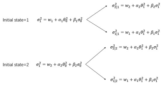
Figure 1. Path Dependency Describe.

At present, there are three main parameter estimation methods used in a Markov state transition model: maximum likelihood estimation, EM algorithm, and Monte Carlo simulation (MCMC). An MCMC algorithm requires extensive of computation and takes a long time in the sampling process, but because this method combines the prior distribution of parameters and the information of data, it samples parameters iteratively. When the collected samples reach the stability of a Markov chain, the convergence parameter can be used as the basis of parameter estimation. In this paper, the MCMC method is used to estimate the parameters of the model by taking the hidden-state variables as the parameters of the model.

3.2. MCMC Estimate

We have to estimate two sets of parameters: (1) transition probability ${\tau }_{11},{\tau }_{22}$ and (2) other parameters in MS-GARCH {${\alpha }_i,{\beta }_i,w_i,i=1,2$}. We follow the Gibbs method in [10] to estimate transition probability τ_11,τ_22,andusea Griddy–Gibbs to estimate other parameters. Although this method is time consuming, because it does not specify the posterior density form of sampling, sampling can be more extensive.

According to [10], we have to estimate four transition probabilities: τ_11,τ_22,τ_12, and τ_21. However, we can divide them into two groups (τ_11,τ_12.) and (τ_22,τ_21.) and use their relationship to solve them:

$${\tau }_{11}+{\tau }_{12}=1$$

$${\tau }_{22}+{\tau }_{21}=1$$

For the remaining parameters, we use a Griddy–Gibbs, an advanced method of Gibbs. A detailed solution can be viewed in [10].

Ultimately, the complete steps of MCMC estimation are shown in Figure 2.

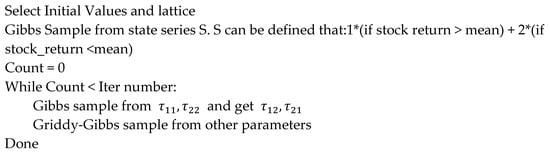
Figure 2. Pseudo code of MCMC.

3.3. Risk Measure

3.3.1. Value at Risk (VaR)

For a long time, the most commonly used risk measurement method for financial institutions has been VaR; that is, given the confidence level Ꮂ and time period t, in time period t a with probability of 1-β, the upper limit of possible losses of a portfolio. If the loss of portfolio can be represented by f(x,S), then $x \in R^n$ presents the portfolio and $S \in R^d$ has the probability density function p(S). Therefore, for portfolio x, we receive the following function for the upper limit of loss α:

$$\phi \left(x,\alpha \right)=\underset{f\left(x,s\right)\le \alpha }{\overset{}{{\displaystyle \int }}}p\left(S\right)dS$$

If p(S) is continuous and $\phi \left(x,\alpha \right)$ is continuous almost everywhere for α, then we can get:

$${\alpha }_{\beta }\left(x\right)=\inf \left\{\alpha \in R:\phi \left(x,\alpha \right)\ge \beta \right\}$$

where α is the parameter of $\phi \left(x,\alpha \right)$ and β is the confidence level.

3.3.2. Condition Value at Risk (CVaR)

However, in practical applications, VaR, a risk-measurement method, exposes its limitations, including (a) a lack of subadditivity and convexity; (b) that the yield is required to follow normal distribution; and (c) that there may be multiple local minimum values when minimizing the problem, which does not meet the requirements of risk ‘consistency’.

Then came another method of risk measurement: conditional value at risk CVaR. Similarly, given the confidence level β and time period t, under the condition that the loss of the portfolio is greater than the corresponding VaR value, the loss of the portfolio is expected, and we get:

$${\phi }_{\beta }\left(x\right)={\left(1-\beta \right)}^{-1}{{\displaystyle \int }}_{f\left(x,s\right)\ge {\alpha }_{\beta }\left(x\right)}^{}f\left(x,s\right)p\left(S\right)dS$$

The optimization problem with CVaR as the optimization objective is convex.

4. Experiments and Analysis

4.1. Data Selection

We choose the fuel oil futures under the energy and chemical futures of Shanghai Futures Exchange as the research object. Data are available from https://www.shfe.com.cn/.The initial date of the data is from 25 August 2004 to 26 July 2022. The statistical values of the data indicators are as follows (Table 1 and Figure 3):

Table 1. Description of Data.

N	Mean	Maximum
4170	3480	5655

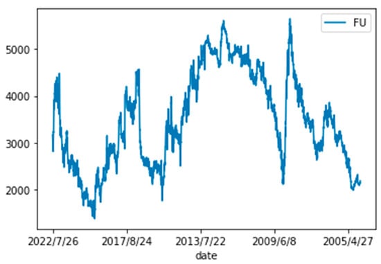
Figure 3. Raw Data Plot.

4.2. ADF Test

In mathematics, a stationary random process or a strictly stationary random process, also known as a narrow stationary process, is a random process whose probability distribution at a fixed time and location is the same as that at all other times and locations; that is, the statistical characteristics of a random process do not change with the passage of time. In this way, the parameters of mathematical expectation and variance do not change with time and location.

In theory, there are two kinds of stationarity: strict stationarity and wide stationarity. In practical application, wide stationarity is used more. The mathematical definition of wide stability is: for time series $y_t$, if for any t, K, m, it satisfies

$$E\left(y_t\right)=E\left(y_{t+m}\right)$$

$$cov\left(y_t,y_{t+k}\right)=cov\left(y_{t+m},y_{t+m+k}\right)$$

then time series $y_t$ is said to be wide and stable.

Stationarity is a necessary condition for an autoregressive GARCH model. Therefore, for time series, we must first ensure that the n-order difference series using autoregression is stable. The sample time series shows the history and current situation of random variables, so the so-called “basic properties” of random variables remain unchanged; that is, the essential characteristics of the sample data time series can continue into the future. We use the mean, variance, and CO (self) variance of the sample time series to describe the essential characteristics of the sample time series. Therefore, we call sample time series whose values of these statistics remain unchanged in the future “stable”. It can be seen that a stable time series refers to the sample time series that can be obtained in the future. We can conclude that its mean value, variance, and covariance must be equal to the sample time series that have been obtained at present. In other words, the mean, variance, and covariance must be constant, otherwise they are unstable. In order to use fuel oil futures data for modeling, we first conducted a unit root test on the closing price of futures, using the ADF test method. Before this could be done, we first needed to take the logarithm of the original price of fuel oil futures, and the data after taking the logarithm can be understood as the change rate of the original data.

The first-order difference of the data after logarithm is shown in Figure 4.

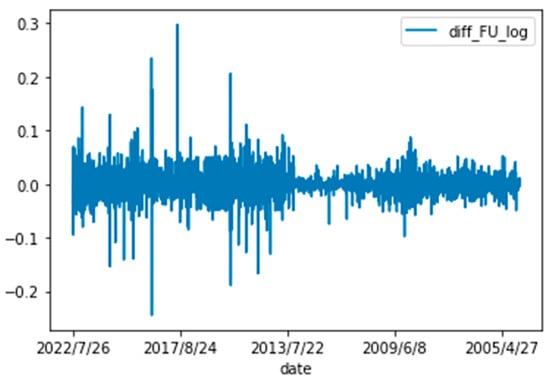
Figure 4. Difference log data.

The unit root test is one of the methods used to test the stability of financial series. The early unit root test uses the DF test [17], but the series often has high-order lag correlation, which destroys the assumption that the random interference term in the DF test is white noise, therefore the augmented Dickey Fuller test (ADF) is used. In this test, the time series is regarded as the autoregressive form of order p (the first-order autoregressive form in the DF test), and the random interference term follows a stationary distribution. In this paper, the ADF test is used to test the stationarity of fuel oil futures data. Taking SiC as the criterion, the maximum lag order is 5. The tests’ statistical measurement results are shown in the table below (Table 2).

Table 2. ADF test result.

Name	Value
Test Statistic	−28.1364
p-value	0.0000
Lags Used	5
Number of Observation Used	4163
Critical Value (1%)	−3.4319
Critical Value (5%)	−2.8622
Critical Value (10%)	−2.5671
Test Statistic	−28.1364
p-value	0.0000

It can be seen that the t statistic is much smaller than the critical values, so the results after the first-order difference are stable. Therefore, we have reason to reject the assumption that there is a unit root in the sequence after the fuel late cargo difference; that is, the sequence satisfies stationarity.

4.3. Parameters Estimate

We used MCMC to estimate the parameters of the MS-GARCH. Gibbs sampling was used in the estimation process. In order to determine the state, we first determined that the sequence value at time t was less than the sequence average value and set it as 1;otherwise, the sequence average value is set as 2. Then Gibbs sampling is used in order to calculate the transition probability and other parameters.

In this paper, 20,000 samples were taken, and an MS-GARCH was used to fit the fuel oil futures. The parameter estimation was obtained as follows (Table 3 and Figure 5).

Table 3. MCMC estimation result.

Name	Mean	Std
${\alpha }_1$	−8.4272	0.01903
${\alpha }_2$	3.5715	0.0097
${\beta }_1$	−2.4513	0.0204
${\beta }_2$	0.8787	0.0020
$w_1$	−9.6826	0.0293
$w_2$	−2.4768	0.0066
${\tau }_{11}$	0.3665	0.0006
${\tau }_{22}$	0.6771	0.0011

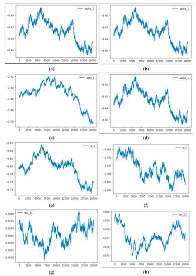
Figure 5. MCMC result.

MS-GARCH divides the fuel oil futures sequence into two state models which correspond to high volatility and low volatility, respectively.

4.4. CVaR Estimate

Therefore, after the parameters’ estimation with MCMC, we used the estimator as the true parameters to calculate the conditional VaR of the hedging strategy of an airline company. The CVaR value of the hedging strategy can be obtained by bringing the parameters estimated by MCMC into an MS-GAECH model. According to our choice of a 95% confidence level, the CVaR estimation results are as follows (Table 4):

Table 4. CVaR Estimate Results.

Position	Maximum	Minimum	Mean	Std
long	4802.12	1205.56	2501.01	527.48
short	4983.58	1307.67	2672.98	672.69

References

- Casella, G.; George, E. Explaining the Gibbs Sampler. Amer. Stat. 1992, 46, 167–174. [Google Scholar]
- Ederington, L.H. The hedging performance of the new futures markets. J. Financ. 1979, 34, 157–170. [Google Scholar] [CrossRef]
- Hou, Y.; Li, S. Hedging performance of Chinese stock index futures: An empirical analysis using wavelet analysis and flexible bivariate GARCH approaches. Pac. Basin Financ. J. 2013, 24, 109–131. [Google Scholar] [CrossRef]
- Chang, C.-Y.; Lai, J.Y.; Chuang, I.-Y. Futures hedging effectiveness under the segmentation of bear/bull energy markets. Energy Econ. 2010, 32, 442–449. [Google Scholar] [CrossRef]
- Zhou, J. Hedging performance of REIT index futures: A comparison of alternative hedge ratio estimation methods. Econ. Model. 2016, 52, 690–698. [Google Scholar] [CrossRef]
- Basher, S.A.; Sadorsky, P. Hedging emerging market stock prices with oil, gold, VIX, and bonds: A comparison between DCC, ADCC and GO-GARCH. Energy Econ. 2016, 54, 235–247. [Google Scholar] [CrossRef]
- Philip, D.; Shi, Y. Optimal hedging in carbon emission markets using Markov regime switching models. J. Int. Financ. Mark. Inst. Money 2016, 43, 1–15. [Google Scholar] [CrossRef]
- Hamilton, J.D. A new approach to the economic analysis of nonstationary time series and the business cycle. Econom. J. Econom. Soc. 1989, 57, 357–384. [Google Scholar] [CrossRef]
- Hamilton, J.D.; Susmel, R. Autoregressive conditional heteroskedasticity and changes in regime. J. Econom. 1994, 64, 307–333. [Google Scholar] [CrossRef]
- Bauwens, L.; Preminger, A.; Rombouts, J.V.K. Theory and inference for a Markov switching GARCH model. Econom. J. 2010, 13, 218–244. [Google Scholar] [CrossRef]
- Das, D.; Yoo, B.H. A Bayesian MCMC algorithm for Markov switching GARCH models. Econom. Soc. 2004, 16, 1–16. [Google Scholar]
- Escamilla-Fajardo, P.; Alguacil, M.; García-Pascual, F. Business model adaptation in Spanish sports clubs according to the perceived context: Impact on the social cause performance. Sustainability 2021, 13, 3438. [Google Scholar] [CrossRef]
- Wilmott, P. Paul Wilmott Introduces Quantitative Finance; John Wiley & Sons: Hoboken, NJ, USA, 2007. [Google Scholar]
- Young, M.R. A minimax portfolio selection rule with linear programming solution. Manag. Sci. 1998, 44, 673–683. [Google Scholar] [CrossRef]
- Duffie, D.; Pan, J. An overview of value at risk. J. Deriv. 1997, 4, 7–49. [Google Scholar] [CrossRef]
- Rockafellar, R.; Uryasev, S. Conditional value-at-risk for general loss distributions. J. Bank. Financ. 2002, 26, 1443–1471. [Google Scholar] [CrossRef]
- Engle, R.F.; Granger, C.W.J. Co-integration and error correction: Representation, estimation, and testing. Econom. J. Econom. Soc. 1987, 55, 251–276. [Google Scholar] [CrossRef]
Publisher’s Note: MDPI stays neutral with regard to jurisdictional claims in published maps and institutional affiliations. |
© 2022 by the authors. Licensee MDPI, Basel, Switzerland. This article is an open access article distributed under the terms and conditions of the Creative Commons Attribution (CC BY) license (https://creativecommons.org/licenses/by/4.0/).