Abstract
This study examines the influences of the power structure evolution along the global coffee value chain on coffee spot-futures commodity markets. Specifically, this study aims to analyze the mechanisms and extent to which the coffee spot-futures commodity markets are affected by shifts in the power structure in each phase following the collapse of the ICA from the perspective of price discovery and volatility spillovers by employing the PT–IS and bivariate EGARCH models. This research covers two actively traded coffee types, Arabica and Robusta, and utilizes daily time-series price data over 1990:01–2020:04 for Arabica and over 2008:01–2020:04 for Robusta. The empirical results indicate that coffee spot markets play a dominant role in price discovery for both Arabica and Robusta over all periods, and volatility spillovers occur from the coffee spot market to the futures markets. This study demonstrates to coffee market players that power structure evolutions across coffee’s global value chain have not significantly changed the underlying socio-spatial distribution of the coffee value chain over the post-ICA period. The results further imply that a buyer-driven governance is emerging in the coffee industry and large coffee roasters are beginning to dominate the global coffee value chain. Moreover, large coffee roasters are incentivized to diversify their marketing strategies by considering more market factors as part of their market differentiation strategies. Government interventions are necessary to establish price risk-management mechanisms to protect small-scale coffee growers.
1. Introduction
Coffee is a valuable export commodity for many less-developed countries (LDCs) located in Africa, Southeast Asia, and Latin America. Small-scale growers in low- or middle-income countries, whose livelihoods and incomes are heavily reliant on the global coffee value chain, produce seventy percent of the world’s coffee [1]. Yet, coffee producers, especially small-scale coffee farmers that bear a large share of the risks, have little bargaining power in the global coffee markets. Substantial uncertainties in their income due to highly volatile market prices and changeable power structures limit their incentives to make investments, and thus distort the global coffee value chain and threaten the long-term global coffee supply [1]. There have been numerous investigations into the process of price discovery in the global coffee industry; however, to the best of our knowledge, there has been no study that has examined the influence of power structure evolution on global coffee commodity markets from the perspective of price discovery and volatility spillovers, which are crucial factors for understanding and predicting the evolution of the global coffee industry from a macro-view.
Over 1962–1989, the global coffee market exhibited stable prices due to multi-country quotas from the International Coffee Agreement (ICA). Each coffee exporter was assigned a quota by the International Coffee Organization (ICO) based on its stocks or previous export records. Yet, the ICA collapsed in 1989 due to trade liberalization and the global coffee industry experienced a significant power shift. Since then, the ICO lost its role in assigning quotas and switched this role to promoting intergovernmental cooperation and the sustainability of the coffee economy [2]. Due to this, the power structure of the global coffee industry has evolved from the “ICA Regime Phase” (1962–1989) to the “Liberalization Phase” (1990–2007) with the market-driven differentiation of quality and characteristics [3]. Following that, the next—and current—phase is known as the “Diversification and Reconsolidation Phase” (2008–present), in which large-scale roasters differentiate the markets by offering a range of coffee products [3]. It is inevitable that the evolution of the power structure in the global coffee industry will affect the price and volatility of the coffee spot-futures markets. The collapse of the ICA resulted in unstable coffee prices since coffee exporters were eager to seek new markets without any quota limits. Examining price discovery and volatility spillovers on the coffee spot-futures commodity markets can provide valuable insights into the influences and mechanisms of power shifts in the global coffee value chain with respect to markets and further predict their long-term trends.
The price discovery process for coffee is a significant contributor to the long-run price stability in global coffee markets. The volatility of Arabica and Robusta futures prices is the driver for price volatility in the global coffee markets [1]. Futures prices reflect global supply and demand and traders’ speculative activities, and many coffee roasters and importers consider futures prices as benchmarks for international trade [1]. An efficient price signal provided by price discovery is an essential tool for the direction of coffee production, consumption, and processing [4]. In comparison, volatility spillovers measure the lead–lag relations and reveal how information is transmitted and disseminated between futures and spot markets [4]. The importance of investigating volatility spillovers lies in establishing appropriate hedging strategies and obtaining the ability to forecast prices effectively [5].
From the perspective of price discovery and volatility spillovers, this study aims to investigate the mechanisms and extent to which the spot-futures commodity markets are affected by the shifts in the power structure in each phase following the collapse of the ICA. Moreover, this study discusses the expected role of each type of power structure in the global coffee value chain as manifested from the coffee spot-futures commodity markets based on the empirical results. Specifically, this research tracks the performance and interactions of futures and spot markets in terms of price stability and market efficiency over the post-ICA period. First, we employ the permanent–transitory and information-share (PT–IS) model to explore the price discovery of quality-differentiated coffee. Second, we utilize the exponential generalized autoregressive conditional heteroskedastic (EGARCH) model to study the volatility spillovers for the coffee futures and spot markets.
The changes in power structures in the post-ICA era have had a significant impact on coffee commodity markets, but very few studies are available that provide an overview of these influences. This study seeks to examine the influences of power structures’ revolution on coffee commodity markets. To the best of our knowledge, this is the first study that examines the topic of power structure evolution in the coffee value chain with an empirical analysis of coffee commodity markets. More specifically, this study analyzes the mechanisms and extent to which the coffee spot-futures commodity markets are affected by shifts in power structure in each phase following the collapse of the ICA from the perspective of price discovery and volatility spillover effects by employing the PT–IS and bivariate EGARCH models. The rest of this study is organized as follows: Section 2 discusses the global coffee market and its power structure evolution. Section 3 presents the literature review, discussing the evolution of the power structure, the price discovery analysis, the volatility spillover effects, and the models employed in the literature. In Section 4, we address the data selection and unit root tests with structural breaks. Section 5 discusses the methodologies used to explore price discovery and volatility spillovers. Section 6 reports the empirical results, presents the interpretations, and discusses the findings. Section 7 concludes and provides policy implications.
2. Global Coffee Market and Its Power Structure Evolution
Coffee is a quality-differentiated product; Robusta and Arabica are two widely recognized types of coffee. Arabica coffee is more prevalent in the market and accounts for more than 60% of the total global coffee production. Arabica coffee is widely accepted as the most popular type of coffee in the world with a broad taste range and stronger aroma. The distinctive characteristics of Arabica come from a higher content of lipids and sugar [6]. According to the ICO, Arabica coffee is mainly grown in higher-altitude areas in Latin America and Africa, and it is categorized into three types: Colombian Milds, Brazilian Naturals, and Other Milds. The term “Milds” refers to high-quality Arabica, wherein Colombian Milds are mainly supplied by Colombia, Kenya, and Tanzania; Other Milds are produced in Mexico and Guatemala. The term “Naturals,” also called “hard Arabica,” refers to low-quality Arabica with a harsher taste; Brazilian Naturals are supplied by Brazil and Ethiopia [2].
In comparison, Robusta has only one type with many origins, such as Sub-Saharan Africa, Southeast Asia, and South America, but it is mainly produced in Vietnam [2]. Robusta coffee accounts for less than 40% of global coffee production and ranks as the second most popular coffee in the world. Compared with Arabica, Robusta coffee has a higher caffeine content and its taste is harsher [6]. The distinctive aspect of coffee with a higher caffeine content is that it resists insects and has a higher yield. Accordingly, the price of Robusta is much lower, i.e., around half the price of Arabica. The U.S. Coffee C Futures is the benchmark for the global Arabica coffee market, and the London Robusta Coffee Futures is the benchmark for Robusta coffee. This research investigates the price discovery and volatility spillovers between coffee futures markets for U.S. Coffee C Futures and London Robusta Coffee Futures, and Colombian Milds, Brazilian Naturals, Other Milds, and Robusta spot markets.
Dallas et al. [7,8] proposed four types of power along global value chains: bargaining power, demonstrative power, institutional power, and constitutive power. Bargaining power refers to the firm-to-firm relationship that mainly operates between suppliers and buyers, and demonstrative power refers to a firm’s relationship with a specific supplier that shapes the behavior of all other suppliers along the value chain. Bargaining power and demonstrative power are more frequently exerted at the firm level. Institutional power refers to formally organized collectives that exert significant influence over an industry, such as business associations and multi-stakeholder initiatives. Constitutive power refers to the exertion of existing norms that emanate from the firm- or group-level in an uncoordinated but collective way. This study focuses on institutional power and constitutive power due to their close relationship and significant influence on the coffee spot-futures commodity market. Table 1 compares the characteristics of three evolutionary phases of the global coffee value chain to demonstrate how power has shifted along the chain.

Table 1.
Comparison of the Characteristics for Three Evolutionary Phases.
The “ICA Regime Phase” (1962–1989) refers to a period in which the ICA established comprehensive quotas for the supply of coffee. Apparently, institutional power was primarily in force during the “ICA Regime Phase” and coffee market prices were quite stable during this period. The “Liberalization Phase” (1990–2007) was the period following the collapse of the ICA, characterized by high price volatility and low prices for a considerable period. During this time, institutional power disintegrated, and constitutive power began to take over. Meanwhile, bargaining power and demonstrative power started to emerge across the entire global coffee value chain.
The “Diversification and Reconsolidation Phase” (2008–present) has been ongoing since the global financial crisis of 2008 and continues to this day. This period is characterized by a restructuring of the global value chain across the entire industry that has been initiated by the value chain players themselves. Top coffee roasters, such as Starbucks and Keurig Green Mountain, have explored diversified coffee products with respect to heterogeneity and polycentricity to increase margins. Some examples include carbon-neutral coffee, coffee from micro-regions, coffee with geographic indications, etc. [3]. There is a significant role being played by constitutive power in this situation, as well as bargaining power and demonstrative power in the coffee value chain.
3. Literature Review
Coffee has received considerable attention in the literature over the past few decades due to its nature as an important foreign exchange earner for many LDCs and the significant power structure shifts in its global value chain. The literature review in this study covers two strands: the first strand describes the investigation of the global coffee price volatility and welfare changes resulting from the collapse of the ICA, as well as the evolution of the power structure in the global coffee value chain; the second strand discusses the use of the PT–IS model to investigate the price discovery in coffee futures-spot commodity markets and the application of the EGARCH model to examine price volatility spillovers.
Coffee price volatility and welfare are closely related to the evolution of power structures. The first strand of the study examines the instability of coffee market prices that has resulted from significant structural changes in the global coffee industry during the post-ICA period, as well as the welfare impacts of these changes on coffee producers, processors, and consumers. Mehta and Chavas [10] employed the semi-structural price vector autoregression method to investigate two major questions: whether the ICA created a coffee price cycle, and whether supply responded to price information in the post-ICA period. Their results indicated that the ICA created a coffee price cycle and that the supply response in the post-ICA years was quite weak due to deregulation. Ghoshray [11] further examined the issue of unstable prices for differentiated coffee and concluded that the post-ICA coffee market is highly integrated with an asymmetric price adjustment pattern. Given that coffee importers are prepared to pay premiums for high-quality coffee, price rises and declines for high-quality coffee lead to slower price increases and faster price declines for low-quality coffee, respectively. The above studies indicate that the power structure shift in the post-ICA period led to unstable global coffee prices.
Several studies have examined the welfare changes of participants in the coffee industry in greater detail. Ponte [9] pointed out that the institutional framework in the global coffee chain has changed from a stable institutional framework to an unstable buyer-driven system, which has led to a transfer of benefits from coffee producers to the consuming countries’ operators. Lewin et al. [12] concluded that the share of value for coffee producers in the global coffee chain dropped from around thirty percent in the Mid-1980s to about five percent in the Mid-2000s. In comparison, coffee-processing firms in coffee-consuming countries and multinationals capture larger downstream margins. Similarly, Feleke and Walters [13] found that the welfare of coffee producers will continue to deteriorate as exports expand in the post-ICA period and suggested that coffee producers adopt new marketing strategies, namely, exporting high-quality coffee, differentiating with value-adding activities, and exploring the domestic market. These welfare changes have great influences on coffee players, especially small-scale coffee producers.
To understand the underlying influences of the significant structural changes in the global coffee industry, Grabs and Ponte [3] reviewed and summarized the evolution of power structures and production networks in the global coffee value chain. Their study concluded that the global coffee industry has experienced a significant power structure shift in the past decades; yet, coffee has not changed its underlying socio-spatial distribution along its value chain as it evolved from a relatively uniform product into a highly differentiated, high-margin product. Grabs [14] also investigated the non-state market-driven (NSMD) governance schemes of coffee value chains from the perspective of dynamic power distributions. The study revealed that NSMD governance has become the mainstream power pattern in the global coffee industry, where large roasters with company-owned standards play an increasingly important role. While numerous studies have examined how the coffee industry’s power structure has changed in the past, to the best of our knowledge, there has not yet been a study that has included coffee commodity markets as part of its empirical analysis. The inclusion of coffee commodity markets in empirical analysis can provide additional insights into the change in the power structure of the global coffee industry from the perspectives of price discovery and volatility spillover.
The second strand of the literature incorporates several approaches from the previous studies to investigate the price discovery process. The Permanent–Transitory and Information Share (PT–IS) measure is a well-developed approach used to investigate the price discovery process in financial markets, but it has not been widely utilized in agricultural commodity markets, especially for the coffee industry. The PT–IS method comprises two popular common factor models: PT and IS; however, the IS and PT models are defined differently when used for price discovery. According to Hasbrouck [15], the IS model measures the relative contributions of each market to the variance of the innovations in the common factor. In comparison, the PT model, introduced by Gonzalo and Granger [16], only concerns the error correction process of price movements. They claim that only the permanent shocks in the error correction process, as opposed to the transitory shocks, result in a market disequilibrium. Thus, the PT model measures the contributions of each market to the common factor. Baillie et al. [17] revealed the connection between the IS and PT approaches in the case of a lack of a significant correlation between the error terms that derived from the co-integration equation.
Empirical studies on a limited range of agricultural products have been undertaken to discuss the estimates of volatility spillover effects [18,19,20]. Yet, the GARCH model has been demonstrated to have two major limitations in those studies. First, the non-negativity condition can be violated by the estimation method if the coefficients are negative. Second, the GARCH model restricts coefficients to allow for the influence of logarithmic leverage effects on the conditional variance specification. Alternatively, Nelson [21] introduced the exponential GARCH model (EGARCH) that releases restrictions on the coefficients and allows for leverage effects. The EGARCH method has been extensively utilized in the following studies. Buguk et al. [22] utilized the EGARCH model to test the volatility spillovers in the U.S. catfish supply chain over 1980–2000. The catfish supply chain includes catfish feed, its ingredients, and farm- and wholesale-level catfish. The empirical results detected price volatility spillovers running from feeding materials to catfish feed and farm- and wholesale-level catfish prices. Shihabudheen and Padhi [4] utilized the VECM and EGARCH models to investigate the price discovery and spillovers in Indian futures and spot markets. The results revealed that the futures market plays a major role in price discovery, and the spillover effect consists of the futures market spilling over into the spot market for most commodities.
Utilizing an empirical analysis of price discovery and volatility spillovers, we fill in the gap in the understanding of how and to what extent the global coffee industry’s change in power structure has influenced coffee commodity markets. Considering market awareness and price predictions, the empirical results have significant implications for all participants in the coffee industry, including large coffee roasters, small-scale coffee growers, and futures market traders. In sum, to gain insights for coffee industry participants, it is necessary to utilize the well-developed PT–IS approach to re-examine the price discovery process, and to use the EGARCH model to investigate the volatility spillover in the coffee spot-futures commodity markets.
4. Data Selection and Unit Root Tests with Structural Breaks
4.1. Data Selection
This study utilizes daily time-series price data to test price discovery with regard to three Arabica coffees and U.S. Coffee C futures over 1990:01–2020:04, as well as Robusta coffee and London Robusta Coffee Futures over 2008:01–2020:04. The data used for the spot prices are from group indicator prices released by the ICO, whereas the data used for the futures prices are from the Intercontinental Exchange (ICE). The ICO group indicator prices are based on spot prices of coffee traded in the U.S., German, and French markets. The weights of each market in calculating the group indicator prices are determined by the average export share to the U.S. and EU (Appendix A). Given that the ICE and the New York Board of Trade (NYBOT) merged in 2007 and formed a new ICE, the futures market price data collected from the ICE includes data incorporated from the NYBOT prior to 2007. Table 2 shows the descriptive statistics of all the price series. Figure 1 and Figure 2 present the historical trends of Arabica and Robusta price series, respectively.
Table 2.
Descriptive Statistics of Continuous Variables a.
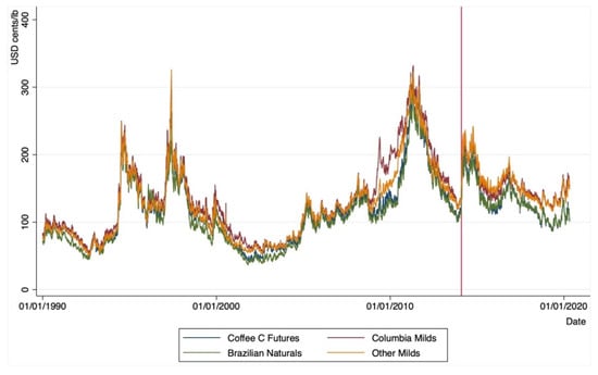
Figure 1.
Price Plots of Three Types of Arabica Coffee and Coffee C Futures 1990:01–2020:04. Source: the ICO and the ICE databases.
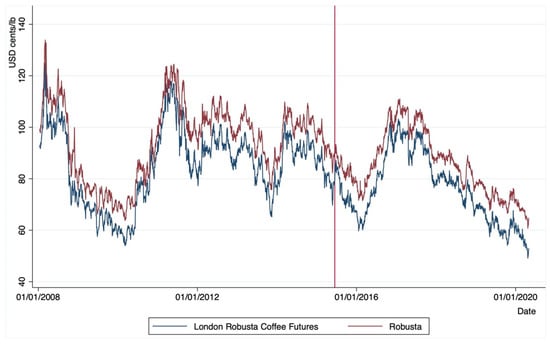
Figure 2.
Price Plots of Robusta Coffee and London Robusta Coffee Futures 2008:02–2020:04. Source: the ICO and the ICE databases.
The prices of U.S. Coffee C Futures fluctuated along with spot market prices over 1990:01–2020:04 (Figure 1). The prices of Arabica coffee reached a high level in the middle of the 1990s and dropped to low levels in the early 2000s. The price drop occurred due to a large expansion in global coffee production, creating large stockpiles and low prices [23]. Then, Arabica coffee prices started to recover at a steady pace until 2011, when the market experienced a dramatic price hike and reached another high-price level in 2011. Figure 2 shows the price movements of Robusta coffee markets over 2008:01–2020:04, wherein the prices of Robusta coffee are more stable than Arabica prices. For example, Arabica coffee doubled in price over 2009–2011, increasing from less than USD 150 cents/lb to more than USD 300 cents/lb. In comparison, Robusta prices stayed around USD 90 cents/lb over the same period.
4.2. Unit Roots Test with Structural Breaks
To avoid spurious regression, we employ the widely used Augmented Dickey–Fuller (ADF) unit root approach [24] to test the stationarity and the Johansen’s cointegration test [25] to detect any cointegration relationships of the price series. Considering the significant influence of complex factors on coffee prices, it is imperative to investigate the structural breaks in coffee price fluctuations. Our analysis of the structural breaks is based on the Wald test, which was developed by Bai and Perron [26] and Andrews and Ploberger [27]. Table 3 presents the empirical results regarding the structural breaks for both Arabica and Robusta price series over the period 1990:01–2020:04. Figure 1 and Figure 2 illustrate the structural break dates using red vertical lines.
Table 3.
Results of Structural Breaks (1990:01–2020:04).
The empirical results show that the estimated break dates for Arabica and Robusta are 6 February 2014 and 15 June 2015, respectively. It appears that the estimated results for both Arabica and Robusta are in line with the market situation regarding global coffee supply and demand. Brazil, which produces over half of the world’s Arabica coffee, suffered a severe drought in 2014, which resulted in a significant decline in the production of coffee. In response to the unexpected external shock, coffee prices have risen significantly and rapidly throughout the world [28]. Vietnam is the primary Robusta planting area, and Robusta coffee has a higher production level due to the sufficient water supply and rainfall during coffee-growing seasons, which has further reduced market prices in the marketing year 2015/2016 [29]. The lags selected for both the stationarity and cointegration tests are derived from the Akaike Information Criterion (AIC) results. Table 4, Table 5 and Table 6 present the results of the ADF test regarding the levels of and at the first-order differences for Arabica coffee over 1990:01–2020:04, 1990:01–2007:12, and 2008:01–2020:04, and for Robusta coffee over 2008:01–2020:04, respectively.
Table 4.
Augmented Dickey–Fuller (ADF) Test Results (1990:01–2020:04).
Table 5.
Augmented Dickey–Fuller (ADF) Test Results (1990:01–2007:12).
Table 6.
Augmented Dickey–Fuller (ADF) Test Results (2008:01–2020:04).
According to the empirical results in Table 4, Table 5 and Table 6, we cannot reject the null hypothesis that all the price series exhibit unit roots at levels, whereas the null hypothesis is overwhelmingly rejected with the first-order differences. The results conform to the condition of the cointegration test with the integration of order one, i.e., I (1).
4.3. Johansen’s Cointegration Test
The purpose of implementing Johansen’s cointegration test [25] is to avoid the potential problem of selecting a dependent variable and to detect cointegrating vectors. Johansen’s test assumes there are no cointegration relationships, and for a long-term cointegration relationship to exist, the null hypothesis must be rejected. Table 7, Table 8 and Table 9 show the results of the Johansen’s test for Arabica and Robusta over the same periods as above. The empirical results reveal that there is at least one cointegrating equation for both Arabica coffee and Robusta coffee at the 5% level, meaning that the Johansen’s test rejects the null hypothesis that there are no cointegrating equations and shows the existence of long-term cointegration relations.
Table 7.
Johansen’s cointegration test results a (1990:01–2020:04).
Table 8.
Johansen’s Cointegration Test Results a (1990:01–2007:12).
Table 9.
Johansen’s Cointegration Test Results a (2008:01–2020:04).
5. The Empirical Model
In this study, the empirical analysis comprises three steps. First, we estimate the VECM outcomes for coffee futures and spot markets as a basis for price discovery and volatility spillover estimates. Second, we calculate the degree of price discovery by utilizing PT–IS measures to determine which market plays a dominant role in the price discovery process. Third, we utilize the EGARCH model to estimate the price dynamics and the direction of the volatility spillovers between coffee futures and spot markets.
5.1. Vector Error Correction Model
The measures of price discovery and volatility spillovers for futures and spot markets are directly derived from the VECM outcomes. The VECM is utilized to investigate the causal relationships and adjustment speeds of futures and spot markets. Each endogenous variable in this model relies on its own lagged values for all the periods, as well as relying on the lagged values of other endogenous variables. The VECM is specified with two pre-requisites for the price series: stationarity and cointegration. The results of the ADF unit root test and Johansen’s cointegration test indicated that the price series satisfied the requirements. The format of the VECM is as follows:
where ΔPt is an i × 1 price vector and η0 is an intercept term that includes an i × 1 vector, in which i equals 4 for Arabica coffee and 2 for Robusta coffee. We include four price series (ΔPCoffee C Futures, ΔPColombian Milds, ΔPBrazilian Naturals, and ΔPOther Milds) for Arabica coffee and two price series for Robusta coffee (ΔPLondon Robusta Coffee Futures and ΔPRobusta) at time t. The ΓiΔPt-i terms explain the short-run relationships for the vectors in the Pt matrix. t denotes the period and k denotes the number of lags. μt is the i.i.d. normal disturbance. ΠPt−k can be rewritten as αβ’Pt−k and the Π matrix explains the long-run relationship among the variables. In this case, the α matrix represents the adjustment speed moving back to long-term equilibrium from a shock. The β matrix incorporates vectors describing the long-term relationship. β’Pt−k is known as the error correction term ECTt−k, which represents the deviation from the equilibrium at period t − k.
5.2. Price Discovery Measures
Various measures have been developed to quantify the relative contributions of the spot and futures markets in the price discovery process, such as PT and IS measures. In the PT–IS model, price discovery is quantified from two different perspectives: the PT model considers how each market contributes to the error correction from permanent shocks, while the IS model emphasizes the relative contributions to the variance of the common trend. For the analysis of the quality-differentiated coffee spot-futures commodity market, the PT–IS model considers two different understandings of price discovery and is based on a mutually supportive process. The PT measure is calculated based on long-run adjustment coefficients derived from the VECM estimation results to measure relative noise avoidance in the price discovery process. Following Baillie et al. [17], the PT measure takes the following form:
where PTf and PTs are PT measures for futures and spot markets, respectively. ξf and ξs are the adjustment parameters for futures and spot markets, respectively. The PT measure utilizes the long-run adjustment coefficient (ξ) derived from the VECM estimation results to test the contributions of the futures and spot markets. The sum of PTf and PTs is always equal to unity so that the greater the adjustment coefficients for one market, the greater the PT measure for the other market. The value intervals for both PTf and PTs are from zero to one. In the extreme case, the futures market dominates the entire price discovery process (PTs = 0) if the spot market offers all adjustments to the equilibrium (ξf = 0), and vice versa.
It should be noted, however, that Equation (2) cannot prevent the adjustment parameters from being negative in many cases, leading to negative PT values. Since the absolute value of the PT measure, rather than its sign, determines the share of contributions to the price discovery process in each market, restrictions that make the factor weights positive resolve the problem of a negative PT measure [30]. We follow Cabrera et al. [31] and Entrop et al. [30] and define the PT measure in the following form:
By capturing the short-term dynamics in the variance-covariance matrix of the VECM residuals, the IS model can serve as an alternative measure of the price discovery process. We follow Hasbrouck [15] and Baillie et al. [17] and define the IS measure as:
where ISf and ISs are IS measures for futures and spot markets, respectively. Ψ represents the long-run impact matrix derived from the VECM estimates. Ω is the variance–covariance matrix of the VECM residuals and M is a transformation from the Cholesky factorization of Ω, such that Ω = MM’. According to Baillie et al. [17], if the error terms that have been derived from the cointegration equation are not correlated, the IS measure takes the following form:
where γf and γs are PT measures for futures and spot markets, respectively; σf and σs are the standard deviations of the coffee spot and futures, respectively. Yet, if the error terms are correlated, Equation (5) does not hold; thus, the IS measure takes the following form:
where , denoting a lower triangular matrix of the Cholesky factorization of Ω = MM’. ρ is the correlation between the innovations.
5.3. The Bivariate EGARCH Model
The volatility spillover effects refer to testing the lead–lag relations in volatilities between coffee futures and spot markets. Nelson’s [21] EGARCH model is used in this study to capture the leverage effects and to avoid the non-negativity restrictions on the estimating parameters. The EGARCH model takes the following form:
where τt2 is the conditional variance, and θ represents the degree of volatility persistence. As θ approaches 1, the volatility and cluster effects become stronger. λ represents the asymmetric parameter (leverage effect) and δ is the symmetric parameter. λ ≠ 0 indicates asymmetry, whereas λ = 0 indicates symmetry. λ < 0 indicates that a negative shock increases volatility, such as a sudden decrease in the coffee supply, whereas λ > 0 indicates that a positive shock increases volatility, such as a sudden increase in coffee demand.
We follow Mahalik et al. [32] and employ the bivariate EGARCH model to investigate the spot-futures commodity market in the following form:
where the unrelated residuals, εs,t−1 and εf,t−1, are obtained from the VECM estimates. The coefficients of the residuals, νf and νs, represent the volatility spillover. They explain whether volatility spillover runs from the futures to the spot or vice versa.
6. Empirical Results and Discussion
As a means of examining the influence of power structures’ evolution on coffee spot-futures commodity markets, this study applied VECM, PT–IS, and EGARCH models to three selected periods of time (1990:01–2007:12, 2008:01–2020:04, and 1990:01–2020:04) to empirically examine price movements, causal relationships, and volatilities across both spot and futures markets. As discussed in Section 3 and Section 5, the VECM model is the basis for the PT–IS and EGARCH analyses, while the reasons for selecting the PT–IS and EGARCH models for price discovery and volatility spillover analyses have already been justified. The following subsections provide the results of the estimates.
6.1. VECM Estimates
Table 10, Table 11, Table 12 and Table 13 present the empirical estimates of the parameters for the price adjustment speed, long-term equilibrium, and short-term causal relations for Arabica over the periods of 1990:01–2020:04, 1990:01–2007:12, and 2008:01–2020:04, respectively, and for Robusta over the period of 2008:01–2020:04. The price adjustment coefficients are quite small in absolute value for both Arabica (0.006 for 1990:01–2020:04, 0.013 for 1990:01–2007:12, and 0.021 for 2008:01–2020:04) and Robusta (0.019 for 2008:01–2020:04) futures market prices and are significant at the 5% level during all three periods. The results reveal slow price adjustment speeds from the short-run shocks to the long-run equilibrium. We have not found any evidence of price adjustment for their spot market prices due to the insignificant coefficients in all three periods.
Table 10.
VECM Estimates for Arabica Coffee (1990:01–2007:12).
Table 11.
VECM Estimates for Arabica Coffee (2008:01–2020:04).
Table 12.
VECM Estimates for Arabica Coffee (1990:01–2020:04).
Table 13.
VECM Estimates for Robusta Coffee (2008:01–2020:04).
The VECM estimates present short-run causal relations. According to the results, there is strong causality between the Arabica spot market prices (Colombian Milds, Brazilian Naturals, and Other Milds) and futures market prices with various lagged periods. Similarly, the VECM results indicate that there is feedback from the futures market prices towards Colombian Milds. However, we have not found short-run causal relationships running from the futures market prices to Brazilian Naturals and Other Milds. In contrast, strong bi-directional short-run causalities between futures and spot market prices were observed for Robusta. Moreover, the empirical results also reveal long-run causal relations between futures and spot market prices for both Arabica and Robusta. In sum, the VECM estimates present both short-run and long-run causal relations running between futures and spot market prices.
6.2. Price Discovery Analysis
Table 14, Table 15 and Table 16 show the empirical estimates of the PT–IS model. According to the PT measure, the contributions of the Arabica coffee futures market are 18.8%, 10.2%, and 38.7% for the period of 1990:01–2020:04; 24.9%, 16.3%, and 30.5% for the period of 1990:01–2007:12; and 18.2%, 7.6%, and 33.7% for the period of 2008:01–2020:04 for Colombian Milds, Brazilian Naturals, and Other Milds, respectively. The IS measure provides similar results, where the contributions to price discovery are 27.0%, 31.0%, and 35.9% for the period of 1990:01–2020:04; 31.1%, 29.7%, and 34.1% for the period of 1990:01–2007:12; and 27.1%, 29.9%, and 29.5% for the period of 2008:01–2020:04 for the three types of coffee above, respectively.
Table 14.
Results of PT–IS Measure for Arabica (1990:01–2007:12).
Table 15.
Results of PT–IS Measure for Arabica and Robusta (2008:01–2020:04).
Table 16.
Results of PT–IS Measure for Arabica and Robusta (1990:01–2020:04).
In comparison, the price discovery process is dominated by spot markets with both PT and IS measures. With the PT measure, the Colombian Milds, Brazilian Naturals, and Other Milds spot markets contribute to price discovery at 81.2%, 89.8%, and 61.3% for the period of 1990:01–2020:04; 75.1%, 83.7%, and 69.5% for the period of 1990–2007; and 81.8%, 92.4%, and 66.3% for the period of 2008:01–2020:04, respectively. Similarly, the IS measure shows the contributions of price discovery at 73.03%, 69.00%, and 64.09% for the period of 1990:01–2020:04; 69.0%, 70.4%, and 66.0% for the period of 1990:01–2007:12; and 72.9%, 70.2%, and 70.6% for the period of 2008:01–2020:04 for Colombian Milds, Brazilian Naturals, and Other Milds, respectively.
In contrast, the PT measure shows that London Robusta Futures contribute 12.3% of the price discovery for the period of 2008:01–2020:04. whereas the Robusta spot market contributes 87.7% for the same period. Similarly, according to the IS estimates, the Robusta futures market contributes 38.9% of the price discovery for the period of 2008:01–2020:04, while the spot market contributes 61.1% for the same period. Combining the findings of both the PT and IS measures, we conclude that Robusta coffee spot markets make a greater contribution to price discovery.
6.3. Volatility Spillover Analysis
Table 17, Table 18 and Table 19 present the empirical results regarding the volatility spillovers from the EGARCH estimates. The findings support the price discovery results in which volatility spillovers transmitted from spot to futures are more significant than the reverse direction due to the larger νf compared with νs over all periods. The larger νf across all spot-futures commodity markets indicates that past innovations in spot markets intensify volatility in the futures markets. Both νf and νs are significant across all spot-futures commodity markets, showing bi-directional volatility spillovers between spot and futures markets over all periods. The magnitude of the spillover coefficient varies from 0.53 for Colombian Milds over all periods to 0.53 for Brazilian Naturals over all periods. Over the periods from 1990:01–2007:12, 2008:01–2020:04, and 1990:01–2020:04, the spillover coefficient for Other Milds varies from 0.49 to 0.56 and 0.55, respectively. During the period of 2008:01–2020:04, the Robusta spot prices have a spillover coefficient of 0.56.
Table 17.
Empirical Results of Volatility Spillovers (1990:01–2007:12).
Table 18.
Empirical Results of Volatility Spillovers (2008:01–2020:04).
Table 19.
Empirical Results of Volatility Spillovers (1990:01–2020:04).
The estimates also indicate that the degree of volatility persistence in the Robusta spot market is similar to the futures market, which is 0.91 vs. 0.89, respectively, over 2008:01–2020:04. Arabica shows a similar and high degree of volatility persistence for Other Milds with coefficients close to unity. For Colombian Milds and Brazilian Naturals, the degrees of volatility persistence in the spot markets are higher than those of the futures market (i.e., 1.00 vs. 0.71 and 0.97 vs. 0.72, over the period of 1990:01–2020:04). The results are similar in the period from 1990:01–2007:12, namely, 1.00 vs. 0.77 and 0.96 vs. 0.81. Yet, the volatility persistence in spot markets is far higher than that of the futures market over 2008:01–2020:04, namely, 0.97 vs. 0.41 and 0.97 vs. 0.39. The results indicate strong volatility and cluster effects for Arabica and Robusta spot-futures commodity market prices, especially over the period of 2008:01–2020:04. The positive λ for the futures and spot market prices of Colombian Milds and Brazilian Naturals in all periods reveals leverage effects, indicating that volatility increases further with positive shocks. In contrast, we have not found leverage effects for Other Milds and Robusta, which had insignificant coefficients in all periods.
The following is a summary of the results. The VECM estimates presented both short-run and long-run causal relations running between coffee futures and spot market prices across all periods of time. Additionally, the VECM estimates provided a basis for the PT–IS and EGARCH models in terms of price discovery and volatility spillovers. According to the PT–IS estimates, the price discovery process is dominated by spot markets rather than futures markets for both the PT and IS measures of Arabica and Robusta across all three periods. The EGARCH estimates indicate that there is a bi-directional spillover of volatility between spot and futures markets, wherein volatility spillover from futures markets to spot markets have stronger statistical significance than the reverse. Moreover, the EGARCH estimation results indicate that the spot-futures prices for Arabica and Robusta are highly volatile and exhibit cluster effects.
Using the perspectives of the coffee commodity markets, we examined the influences of the power structures’ evolution by analyzing price discovery and volatility spillovers across two evolutionary phases: the “Liberalization Phase” (1990–2007) and the “Diversification and Reconsolidation Phase” (2008–present). As far as we are aware, this is the first empirical study to investigate power-structural change in such an empirical manner, and the estimation results contradict our general belief that power-structural changes have significant impacts on the global coffee industry. Contrary to our expectations, both price discovery and volatility spillovers show consistent results during the “Liberalization Phase” (1990–2007) and the “Diversification and Reconsolidation Phase” (2008–present) of the post-ICA period, suggesting that power structures’ revolutions have only a limited influence on coffee commodity prices. These estimation results provide a new perspective on the coffee industry, which may be valuable to all industry participants.
6.4. Discussion of the Findings
Previous studies of the coffee industry over the post-ICA period have focused to a greater degree on price movements and price transmission. A change from a stable institutional framework to an unstable buyer-driven system followed the collapse of the ICA in 1989, resulting in volatile global coffee prices [14]. In view of this, the functions of price discovery and volatility spillovers are more valuable for investigation, which reveals the status of the coffee commodity market’s functioning [33]. Despite significant changes in power structures, our empirical study indicates that coffee commodity markets function well. Further, the results show that over the 2008:01–2020:04 period, the coffee market exhibited a high degree of volatility and cluster effects compared to the 1990:01–2007:12 period. Based on our empirical findings, we concur with Feleke and Walters [13] that the welfare of coffee growers, especially small-scale coffee producers, is highly likely to be impacted by volatile market prices.
A consistent empirical result in price discovery and volatility spillovers for both “Liberalization Phase” (1990–2007) and “Diversification and Reconsolidation Phase” (2008–present) also confirms Grabs and Ponte’s [3] assertion that there has been no significant change in the underlying socio-spatial distribution of the coffee value chain during the post-ICA period. Recent stronger volatility and clustering effects for both Arabica and Robusta indicate a higher degree of financialization of the coffee industry, which is likely due to inter-temporal and cross-market arbitrage by market traders and speculators. A higher degree of volatility and stronger cluster effects could also indirectly confirm Grab’s [14] claim that buyer-driven governance is emerging in the coffee industry. The reason for this is that coffee producers, particularly small-scale producers in LDCs that produce around seventy percent of the world’s coffee, would suffer the most from high price volatility. Large coffee roasters that can differentiate global coffee markets and tolerate price risks are more likely to survive under a buyer-driven market condition. Consequently, large coffee roasters will begin to dominate the global coffee value chain and establish company-owned standards. Moreover, given that spot market prices are playing a dominant role in price discovery, large coffee roasters are encouraged to diversify their marketing strategies by considering more market factors as part of their market differentiation efforts.
7. Conclusions and Implications
This study seeks to examine how power structures’ evolution during the post-ICA period has affected the global coffee value chain from the perspective of price discovery and volatility spillovers. This paper utilizes the PT–IS model to investigate the price discovery process and employs the bivariate EGARCH model to measure volatility spillovers across coffee futures and spot markets. We utilized a dataset covering 1990:01–2020:04 for Arabica and from 2008:01–2020:04 for Robusta. The empirical results show that both Arabica and Robusta coffee spot markets have a dominant role in price discovery and volatility spillover processes.
The empirical analysis of price discovery provides several implications. First, the inefficiency of the coffee futures market in terms of price discovery can be explained by the increasing heterogeneity of coffee products led by large coffee roasters over the post-ICA period. For example, heterogeneous coffee products produced by Starbucks and Keurig Green Mountain could be too differentiated for the U.S. Coffee C futures price to accurately reflect the supply and demand conditions. It is worth noting that price discovery in different coffee-producing regions can be quite diverse. The country-level coffee commodity market has not been well-established in Africa and Southeast Asia, where local producer prices accommodate new information faster. Many market factors can contribute to the role of local producer prices, such as the local market size, the local consumption volume, and the local marketing strategies of coffee-processing firms. The differentiation of markets affords big roasters greater opportunities for market participation, where bargaining power and demonstrative power are expected to take on a more significant role. Still, small-scale coffee growers have little or no market power, and joining local cooperatives could increase their bargaining power among market competition.
Second, the currently diminished role of futures markets in price discovery reveals that the local governments, coupled with global coffee-processing firms, need to devote more resources to help reduce risk for producers, especially small-scale coffee growers. It is imperative that institutional and constitutive power are emphasized as means of protecting small-scale coffee growers. There are several ways that local governments can help producers reduce price risks: (i) establish a warehouse receipt mechanism and invest in corresponding physical infrastructure, such as warehouses for coffee storage and roads for coffee transportation from the farmers to the local warehouse, to increase the flexibility of the time to sell coffee; (ii) establish a country-level export management mechanism, whereby governments can manage the coffee supply based on the dynamics of coffee price movements in the global market; and (iii) build independent marketplaces that decouple the prices from the coffee commodity markets and determine the coffee prices based on quality through auctions or agreements and provide more stable prices for high-quality coffee growers.
The direction of volatility spillovers in spot-futures commodity markets is determined by the ability to accommodate the flow of information. The increase in the information flow in one market due to technology enhancement or trade growth can spill over into other markets, generating price volatility. Given that the coffee spot market is more informationally efficient, the futures market has not been fully developed as a risk-hedging and price-stabilizing instrument since the collapse of the ICA. One reason for this may be the lack of futures market accessibility for coffee farmers that are widely distributed in LDCs with restricted high-quality technology availability. The other reason may come from the low educational level of coffee farmers and traditional conventions of using local producer prices in LDCs. The lack of a futures market as a risk-hedging instrument will in turn restrict the production scale for coffee farmers since expanding production could lead to unbearable risks. The intervention of institutional and constitutive power will help to promote efficiency of commodity markets. Governments and coffee-processing firms are dedicated to cooperating closely so as to promote the development of coffee futures markets.
Yet, both Arabica and Robusta exhibited consistent results in terms of price discovery and volatility spillovers during the “Liberalization Phase” (1990–2007) and the “Diversification and Reconsolidation Phase” (2008–present). This indicates that the evolution of power structures within the global coffee value chain has had very limited influence on spot-futures commodity markets. The results indicate that price movements in the coffee spot market are independent and market-driven, which implies that external shocks caused by structural changes in the coffee industry should be considered less influential than market factors when making business decisions for coffee-processing companies.
There are three primary limitations to this study. First, the availability of price data for this study was relatively limited. There are several local coffee futures markets around the world, such as the Coffee Futures Exchange of India (CFEI) and the Ethiopian Commodity Exchange (ECX), but we considered only the Coffee C Futures prices due to the availability of data. Additionally, this study utilized the group indicator prices provided by the ICO for the spot markets, which were insufficient for distinguishing green coffee from roasted coffee and discriminating between regions. For example, prices in different regions can differ substantially; a roasted coffee spot price in Germany may differ significantly from the spot price in Vietnam, resulting in biased empirical results. For precise prediction, a dataset differentiated by region and category is required. Second, there is space to improve the models selected for price discovery and volatility spillovers. Some studies hold different points of view regarding model selection for investigating commodity market functions and characteristics, including with respect to price discovery, volatility spillovers, market efficiency, market integration, and causality relationships. Other than the models utilized in our study, the econometric methods employed for testing and comparison refer to the FCVAR model [34], ARDL bounds testing [35], variance ratio tests [36,37], bivariate ARFI-FIGARCH [38], dynamic ordinary least squares (DOLS) and fully modified ordinary least squares (FMOLS) analyses [39], the cost-of-carry model [40], the information leadership model [40], etc. Additional reasonable models for estimating price discovery and volatility spillovers should be tested and compared for further analysis. Third, the power structure revolution could be considered as only one aspect of the consistent mechanisms of coffee commodity price discovery and volatility spillovers. Considering the limitations with respect to data, some other aspects, such as changes in the production scale and consumer preference, have not been taken into consideration. Further studies on the factors that may affect the coffee commodity markets can be implemented.
This study is expected to have a broad and practical scope for future research and practical applications. Since coffee is a widely traded agricultural commodity with a large base of growers, investigating power structure changes from the perspectives of coffee production, consumption, trade, and price transmission should be of great value. With large coffee roasters playing a greater role in the global coffee supply chain, it is necessary to examine the change in the production type and its corresponding supply–response analysis. There is also a key component of research on the global coffee industry that involves trade, as volatile coffee prices after the collapse of the ICA should be closely related to the global trade networks for coffee. The consideration of how the coffee trade volume fluctuates with the changes in futures and spot coffee prices is of great interest and value.
The possible negative effects of the COVID-19 pandemic and the shrinking coffee demand worldwide could have forced large coffee roasters to squeeze their margins. An analysis of the responses of futures and spot markets to dramatic price movements and how price is vertically transmitted in the coffee industry due to exterior shocks would be interesting. Moreover, since price discovery can be quite diverse in different regions, a further investigation of price discovery in each coffee-producing region, and the futures market’s role in determining coffee-processing firms’ market power, could provide insights for coffee growers and coffee-processing firms with respect to business-related decision making. A major limitation of the above studies is that coffee is a commodity that differs across regions in terms of the type of production, the coffee category, and the establishment of spot and futures markets. Data on local prices and trade can be obtained through cooperation with local governments and large-scale coffee roasters.
Author Contributions
Conceptualization, W.Z.; methodology, W.Z.; software, W.Z.; validation, W.Z., S.S. and M.R.; formal analysis, W.Z; investigation, W.Z; resources, W.Z; data curation, W.Z; writing—original draft preparation, W.Z; writing—review and editing, S.S. and M.R.; visualization, W.Z.; supervision, S.S. and M.R.; project administration, S.S. and M.R.; funding acquisition, W.Z. All authors have read and agreed to the published version of the manuscript.
Funding
This research is supported by Chinese Universities Scientific Fund, grant number 2022TC118.
Institutional Review Board Statement
Not applicable.
Informed Consent Statement
Not applicable.
Data Availability Statement
The data are available upon request.
Acknowledgments
The authors would like to thank the editors and the reviewers. Wei Zhang acknowledges the support from the International Coffee Organization and China Agricultural University. Sayed Saghaian acknowledges the support from the United States Department of Agriculture, National Institute of Food and Agriculture, Hatch project No. KY004063, under accession number 7002927.
Conflicts of Interest
The authors declare no conflict of interest.
Appendix A
Table A1.
The Weights of Each Market Used to Calculate the Group Indicator Prices.
Table A1.
The Weights of Each Market Used to Calculate the Group Indicator Prices.
| Groups | EU | U.S. |
|---|---|---|
| Colombian Milds | 0.43 | 0.57 |
| Brazilian Naturals | 0.61 | 0.39 |
| Other Milds | 0.73 | 0.27 |
| Robusta | 0.82 | 0.18 |
Source: the ICO.
References
- USAID (U.S. Agency for International Development). Price Risk Management in the Coffee and Cocoa Sectors; USAID: Washington, DC, USA, 2019.
- Li, X.L. Price Analysis Under Production Differentiation in Green Coffee Markets (No. 44). Doctoral Thesis, University of Kentucky, Lexington, KY, USA, 2016. Available online: https://uknowledge.uky.edu/agecon_etds/44 (accessed on 5 June 2022).
- Grabs, J.; Ponte, S. The evolution of power in the global coffee value chain and production network. J. Econ. Geogr. 2019, 19, 803–828. [Google Scholar] [CrossRef]
- Shihabudheen, M.T.; Padhi, P. Price discovery and volatility spillover effect in Indian commodity market. Indian J. Agric. Econ. 2010, 65, 902-2016-67367. [Google Scholar]
- Apergis, N.; Rezitis, A. Agricultural price volatility spillover effects: The case of Greece. Eur. Rev. Agric. Econ. 2003, 30, 389–406. [Google Scholar] [CrossRef]
- Khapre, Y.; Kyamuhangire, W.; Njoroge, E.K.; Kathurima, C.W. Analysis of the Diversity of Some Arabica and Robusta Coffee from Kenya and Uganda by Sensory and Biochemical Components and Their Correlation to Taste. IOSR J. Environ. Sci. Toxicol. Food Technol. 2017, 11, 39–43. [Google Scholar]
- Dallas, M.; Ponte, S.; Sturgeon, T. A Typology of Power in Global Value Chains; Working Paper in Business and Politics 92; Copenhagen Business School, Department of Business and Politics: Frederiksberg, Denmark, 2017. [Google Scholar]
- Dallas, M.; Ponte, S.; Sturgeon, T. Power in global value chains. Rev. Int. Political Econ. 2019, 26, 666–694. [Google Scholar] [CrossRef]
- Ponte, S. The latte revolution? Regulation, markets and consumption in the global coffee chain. World Dev. 2002, 30, 1099–1122. [Google Scholar] [CrossRef]
- Mehta, A.; Chavas, J.P. Responding to the coffee crisis: What can we learn from price dynamics? J. Dev. Econ. 2008, 85, 282–311. [Google Scholar] [CrossRef]
- Ghoshray, A. On price dynamics for different qualities of coffee. Rev. Mark. Integr. 2009, 1, 103–118. [Google Scholar] [CrossRef]
- Lewin, B.; Giovannucci, D.; Varangis, P. Coffee markets: New paradigms in global supply and demand. In World Bank Agriculture and Rural Development Discussion Paper; The World Bank: Washington, DC, USA, 2004; Volume 3. [Google Scholar]
- Feleke, S.T.; Walters, L.M. Global Coffee Import Demand in a New Era: Implications for Developing Countries. Rev. Appl. Econ. 2005, 1, 223–237. [Google Scholar]
- Grabs, J. The Rise of Buyer-Driven Sustainability Governance: Emerging Trends in the Global Coffee Sector. Available online: http://ssrn.com/abstract=3015166 (accessed on 15 July 2022).
- Hasbrouck, J. One security, many markets: Determining the contributions to price discovery. J. Financ. 1995, 50, 1175–1199. [Google Scholar] [CrossRef]
- Gonzalo, J.; Granger, C. Estimation of common long-memory components in cointegrated systems. J. Bus. Econ. Stat. 1995, 13, 27–35. [Google Scholar]
- Baillie, R.T.; Booth, G.G.; Tse, Y.; Zabotina, T. Price discovery and common factor models. J. Financ. Mark. 2002, 5, 309–321. [Google Scholar] [CrossRef]
- Bollerslev, T. Generalized autoregressive conditional heteroskedasticity. J. Econom. 1986, 31, 307–327. [Google Scholar] [CrossRef]
- Engle, R.F. Autoregressive conditional heteroscedasticity with estimates of the variance of United Kingdom inflation. Econometrica J. Econom. Soc. 1982, 50, 987–1007. [Google Scholar] [CrossRef]
- Rezitis, A.N. Volatility spillover effects in Greek consumer meat prices. Agric. Econ. Rev. 2003, 4, 29–36. [Google Scholar]
- Nelson, D.B. Conditional heteroskedasticity in asset returns: A new approach. Econom. J. Econom. Soc. 1991, 59, 347–370. [Google Scholar] [CrossRef]
- Buguk, C.; Hudson, D.; Hanson, T. Price volatility spillover in agricultural markets: An examination of US catfish markets. J. Agric. Resour. Econ. 2003, 28, 86–99. [Google Scholar]
- Boydell, H. What Should We Have Learned from The 2001 Coffee Price Crisis? Perfect Daily Grind. 25 September 2018. Available online: https://www.perfectdailygrind.com/2018/09/what-should-we-have-learned-from-the-2001-coffee-price-crisis/ (accessed on 15 July 2022).
- Dickey, D.A.; Fuller, W.A. Likelihood ratio statistics for autoregressive time series with a unit root. Econom. J. Econom. Soc. 1981, 49, 1057–1072. [Google Scholar] [CrossRef]
- Johansen, S.; Juselius, K. Maximum likelihood estimation and inference on cointegration—With applications to the demand for money. Oxf. Bull. Econ. Stat. 1990, 52, 169–210. [Google Scholar] [CrossRef]
- Bai, J.; Perron, P. Estimating and testing linear models with multiple structural changes. Econometrica 1998, 66, 47–78. [Google Scholar] [CrossRef]
- Andrews, D.W.; Ploberger, W. Optimal tests when a nuisance parameter is present only under the alternative. Econom. J. Econom. Soc. 1994, 62, 1383–1414. [Google Scholar] [CrossRef]
- Stromberg, J. Why You’re Going to be Paying More for Coffee Soon. Vox. 2014. Available online: https://www.vox.com/2014/5/30/5746272/why-youre-going-to-be-paying-more-for-coffee-soon (accessed on 20 July 2022).
- Tran, Q.; Ward, M. Vietnam Coffee Semi-Annual. Global Agricultural Information Network Report, USDA-FAS. 2015. Available online: https://apps.fas.usda.gov/newgainapi/api/report/downloadreportbyfilename?filename=Coffee%20Semi-annual_Hanoi_Vietnam_11-18-2015.pdf (accessed on 3 August 2022).
- Entrop, O.; Frijns, B.; Seruset, M. The determinants of price discovery on bitcoin markets. J. Futures Mark. 2020, 40, 816–837. [Google Scholar] [CrossRef]
- Cabrera, J.; Wang, T.; Yang, J. Do futures lead price discovery in electronic foreign exchange markets? J. Futures Mark. Futures Options Other Deriv. Prod. 2009, 29, 137–156. [Google Scholar] [CrossRef]
- Mahalik, M.K.; Acharya, D.; Babu, M.S. Price discovery and volatility spillovers in futures and spot commodity markets: Some empirical evidence from India. IGIDR Proc./Proj. Rep. Ser. 2009, PP-062-10. Available online: www.igidr.ac.in/pdf/publication/PP-062-10.pdf (accessed on 22 September 2022).
- International Coffee Organization (ICO). The Role of the Coffee Futures Market in Discovering Prices for Latin American Producers; International Coffee Council 122nd Session: London, UK, 2018. [Google Scholar]
- Dolatabadi, S.; Nielsen M, Ø.; Xu, K. A fractionally cointegrated VAR analysis of price discovery in commodity futures markets. J. Futures Mark. 2015, 35, 339–356. [Google Scholar] [CrossRef]
- Pradhan, R.P.; Hall, J.H.; Du Toit, E. The lead–lag relationship between spot and futures prices: Empirical evidence from the Indian commodity market. Resour. Policy 2021, 70, 101934. [Google Scholar] [CrossRef]
- Go, Y.H.; Lau, W.Y. Investor demand, market efficiency and spot-futures relation: Further evidence from crude palm oil. Resour. Policy 2017, 53, 135–146. [Google Scholar] [CrossRef]
- Mohanty, S.K.; Mishra, S. Regulatory reform and market efficiency: The case of Indian agricultural commodity futures markets. Res. Int. Bus. Financ. 2020, 52, 101145. [Google Scholar] [CrossRef]
- Bhaumik, S.; Karanasos, M.; Kartsaklas, A. The informative role of trading volume in an expanding spot and futures market. J. Multinatl. Financ. Manag. 2016, 35, 24–40. [Google Scholar] [CrossRef]
- Inoue, T.; Hamori, S. Market efficiency of commodity futures in India. Appl. Econ. Lett. 2014, 21, 522–527. [Google Scholar] [CrossRef]
- Bohl, M.T.; Siklos, P.L.; Stefan, M.; Wellenreuther, C. Price discovery in agricultural commodity markets: Do speculators contribute? J. Commod. Mark. 2020, 18, 100092. [Google Scholar] [CrossRef]
Publisher’s Note: MDPI stays neutral with regard to jurisdictional claims in published maps and institutional affiliations. |
© 2022 by the authors. Licensee MDPI, Basel, Switzerland. This article is an open access article distributed under the terms and conditions of the Creative Commons Attribution (CC BY) license (https://creativecommons.org/licenses/by/4.0/).