Sources of SMEs Financing and Their Impact on Economic Growth across the European Union: Insights from a Panel Data Study Spanning Sixteen Years

Abstract

Getting access to sufficient funding is the keystone for the development of any business, but especially for small and medium enterprises (SMEs). These economic entities are crucial players in the global economy since they include almost 90% of companies, provide jobs for nearly 50% of the global workforce, and enhance long-term economic growth. In this context, our study explores important sources concerning the financing of small and medium enterprises and their impact on economic growth during the period 2005–2020 with data from SMEs covering the 28 countries belonging to the European Union. The set of predictors included Strength of legal rights index, Days sales outstanding, Bad debt loss, Interest rate, Bank support, Business angels, Private lenders, and Public support. The set of dependent variables included Cost of loans, Equity fund, GDP growth rate, and Value added growth rate. Our methodological approach was complex, it considered a panel data analysis with a first-difference generalized method of moments estimator and a multiplex time series analysis. The novelty of the study resides in combining the two methods in order to investigate significant drivers of economic growth across the EU. Empirical results showed that economic growth was mainly triggered by predictors such as Interest rate, Business angels, Bank support, and Public support. Moreover, the valuable mathematical insights elicited by the multiplex time series analysis suggested that European economies cooperated intensively through SME activities. Based on our empirical results, national and regional authorities should enact adequate policies to support business endeavors of small and medium enterprises.

1. Introduction

Economic markets and economic activities in general entail a multitude of risks deriving from macroeconomic and microeconomic factors, but also from political and social contexts [1,2,3,4,5,6].

The financing of small and medium enterprises (SMEs) falls into the category of microeconomic factors that impact global and regional economic markets for a variety of reasons. For a comprehensive definition of the “small and medium enterprises” concept, one can check the User Guide to the SME Definition, provided by the European Union [7]. First, SMEs are considered the engine of the global economy (and regional economies) since they make up almost 90% of companies, hire about 50% of worldwide human resources, and are estimated to provide around 600 million jobs by the year 2030 [8,9]. When it comes to OECD members, SMEs represent 99% of businesses, employ 70% of the official workforce, and yield around 50% of GDP (the latter being applicable in the case of high-income countries) [10,11]. Second, the economic activities of SMEs are catalysts of economic growth for all countries around the word [12,13,14]. In this context, to secure sustainable economic growth in the long run, national authorities are called to design economic policies that facilitate the access of SMEs to suitable financial sources. Since financing is regarded as the lifeblood of economic activities, SMEs can survive, develop, and thrive on the market only when granted financial support. As a case in point, decision-makers can incentivize SMEs to access financing by subsidizing interest rate payments, granting them preferential tax regimes (even tax exemption status for certain periods), or by subsidizing wages for certain categories of employees (e.g., recent college graduates, senior citizens, disadvantaged groups). Third, within a global framework market with rapid changes in terms of information and technology, business management, characteristics of social interactions, education, cultural norms, and political precepts, the sector of small and medium enterprises represents a basic feature for the development of a modern, dynamic, knowledge-based economy. Fourth, SMEs are deemed valuable sources of entrepreneurial skills and innovation, aside from being a factor of social and economic cohesion [15,16]. Fifth, SMEs feature a flexible development strategy by responding quickly to the intensive competitiveness of international markets and adapting rapidly to cyclical changes of the global economy [17].

When it comes to the European Union, the economic activity of SMEs has registered considerable growth during the past decade. For instance, in 2018, the EU-28 countries had roughly 25 million SMEs, among which 93% were micro-SMEs. In 2019, SMEs accounted for 60% of the increase in value added across member states. For that matter, official statistics reported that most of this increase was due to less knowledge-intensive industries.

A study conducted by McKinsey [11]—a renowned global management consulting firm—listed several challenges and opportunities faced by SMEs nowadays, such as digitalizing business activities, strategic internationalization, amassing critical talent (e.g., digital, in-house R&D expertise, possessing knowledge regarding the regulatory environment overseas), and contributing substantially to the decarbonization process, which aims to reach net-zero greenhouse gas emissions in the EU by 2050.

As a World Bank report perfectly noticed, funding is the Achilles’ heel of SME growth and the second top-rated factor hindering their economic activities, particularly in numerous developing and emerging economies [8]. Indeed, SMEs are often faced with market imperfections, which trigger multiple difficulties in obtaining capital or formal credit, especially in the start-up phase. In this context, improving the capacity of SMEs to access financing is a sine qua non element. Hence, we deem that analyzing how financing sources of SMEs influence the levels of economic growth is both timely and relevant for the regional economy. In this sense, insights from the evolution of economic growth across European states might assist other regional and national authorities interested in boosting economic growth via SME funding sources.

Our sample included data from small and medium enterprises spanning the 28 nations that belonged to the European Union. The period of analysis comprised 16 years (i.e., 2005–2020). We focused on this particular time interval because it regarded a challenging period after the global financial crisis, when the financing process of all businesses (including small and medium enterprises) slipped on a decreasing trend for a period of time before regaining their ascending direction.

With respect to methodology, we favored a multiple research approach with panel data modeling using the first-difference generalized method of moment (GMM) estimator and mathematical modeling via multiplex time series analysis.

The novelty of our research study resides in the fact that panel data analysis and multiplex time series analysis joined forces to elicit significant drivers of economic growth across the European Union by focusing on small and medium enterprises.

The article is structured as follows. Section 2 reports key insights from some of the relevant studies on SME financing. Section 3 details the variables of interest and research hypotheses. Section 4 presents the econometric models and empirical results. Section 5 brings mathematical perspectives on the relationships between SME funding sources that shape economic growth. Section 6 concludes on the most important empirical results, draws relevant policy implications, and announces potential research directions.

2. Literature Review

The following paragraphs point out insights from the current economic literature on how funding granted to small and medium enterprises influences economic growth. In this sense, scientific studies, reports, and official statistics from global and regional bodies, along with media articles, were surveyed in order to elicit the impact of these factors.

SMEs make a huge contribution to national and regional economies even though they are categorized as “small” or “medium.” As Richard Branson, a savvy British entrepreneur and founder of one of the most recognizable brands in the world, once said, a big business starts small [18]. In this context, SMEs can make their market debut as micro-companies having at most 10 employees, but, with time, they can become leaders of their industries. Ultimately, SMEs can substantially drive the levels of economic growth. Since any business activity needs financial resources to properly function and develop, we deem it is relevant and timely to list some of the most important funding sources for SMEs and to examine how these sources drive economic growth.

The extant literature on SMEs reports numerous scientific studies that focused on funding sources. In this regard, stressing the fact that over 96% of Asian businesses are SMEs in a “bank-dominant” economy, Yoshino and Taghizadeh-Hesary [19] discussed the challenges faced by these companies when applying for more affordable bank funding.

Comprehensive reports from international bodies have also addressed the problem of SME funding, which is omnipresent irrespective of the state of economic development. According to an OECD report on growth and job creation [14] (p. 15), the organization mentions some of the most used funding methods, such as bank loans, external equity, factoring, leasing, private equity, overdrafts, retained earnings, and venture capital. The same report emphasizes the fact that the nature of funding sources changes with the development state of the business. Hence, the majority of new SMEs are generally funded through personal savings, whereas only a small part benefits from banks loans.

In this sense, Hossain et al. [20] focused on the connection between SME growth and local financial development based on data from 1,084 SMEs in manufacturing industries. Kapitsinis et al. [21] examined Welsh small and medium enterprises and reported a low demand and insufficient supply of equity investment. Regarding the Bulgarian market and the effectiveness of energy-support schemes granted to SMEs by the European Union, Nigohosyan et al. [22] found that large companies were more cost-effective. In light of their empirical results, the authors suggested that public authorities should better design energy-efficiency support schemes that are grounded on solid assessment criteria of SMEs and internal benchmarking.

Hasan et al. [23] investigated the willingness of banks to support the economic activities of small and medium enterprises. Empirical results showed that local banks were the most solid supporters of SME business endeavors as opposed to foreign banks. Mkhaiber and Werner [24] observed the impact of the size of the bank granting loans to smaller businesses. Starting from their empirical assessments, the authors concluded that bank size establishes an indirect connection with the willingness to offer financial support, as expected.

By means of bibliometric and statistical analysis, Ciampi et al. [25] systematically reviewed 100 research studies published in top-tier outlets on the topic of SME default prediction modeling, considering the time span 1986–2019. The authors emphasized various avenues for future research in order to assist scholars interested in the evolution of SME activities.

Eldridge et al. [26] analyzed how equity crowdfunding would influence innovation and growth opportunities of small and medium enterprises in the United Kingdom. The empirical results elicited the idea that crowdfunding did not have a relevant impact on SMEs’ innovation capacities. At the same time, crowdfunding did play a positive role in the growth of SMEs.

Considering innovation as a relevant factor for SME development, Mina et al. [27] studied which factors impede this development. According to their results, funding was granted to SMEs that demonstrated growing potential, patenting capacities, and experience with venture capital funding.

Using data from SMEs operating in the Korean market, Kim and Cho [28] examined the effects of funding on company performance and efficiency. Their results revealed that company performance was positively shaped by internal and institutional funding. At the same time, financial results were negatively impacted by other capital. In terms of efficiency, this was negatively affected by institutional funds but positively impacted by internal funds. In addition, institutional funds did mitigate company growth.

Last but not least, Wang et al. [29] studied how trade credit shapes the company performance of SMEs. Analyses conducted on data retrieved from 74,036 economic entities during the period 2006–2015 showed that performance increased due to trade credit.

3. Variables of Interest and Research Questions

The 28 countries included in our sample were the following: Austria, Belgium, Bulgaria, Croatia, Czech Republic, Cyprus, Denmark, Estonia, Finland, France, Germany, Greece, Hungary, Ireland, Italy, Latvia, Lithuania, Luxembourg, Malta, the Netherlands, Poland, Portugal, Romania, Slovakia, Slovenia, Spain, Sweden, and the United Kingdom. Our data were retrieved for the period 2005–2020.

To pursue the aim of this study, we selected the following dependent variables from the Eurostat database [30]:

• Cost of loans (CL): measures the borrowing costs for small loans as compared to large loans. It is expressed as a percentage.
• Equity fund (EF): measures equity funding available for new and developing companies. It is expressed on a Likert scale from 1 to 5.
• Gross domestic product growth rate (GDPGR): measures the percentage growth rate at market-based prices on constant local currency. It is computed by dividing the current GDP size to the GDP size from the previous year.
• Value added growth rate (VAGR): measures the percentage growth rate for value added in services based on local currency. It is computed by dividing the current GDP size to the GDP size from the previous year.

In terms of independent variables, we considered the following indicators. Again, Eurostat was the variable source:

• Strength of legal rights index (SLRI): measures the degree to which borrowers’ and lenders’ rights are protected by collateral and bankruptcy laws (namely, it expresses lending facilitation). The index takes values from 0 to 12, with higher scores showing that access to credit is facilitated by better-designed laws.
• Days sales outstanding (DSO): measures the number of days in which customers pay invoices issued by companies.
• Bad debt loss (BDL): measures the size of receivables that must be written off for not being paid. It is computed as a percentage in overall company turnover.
• Interest rate (IR): measures the interest rate average set for small loans. It is expressed as a percentage.
• Bank support (BS): measures a bank’s lending availability. It is expressed as a percentage of respondents who signaled a deterioration in accessing a loan.
• Business angels (BA): measures funding available from business angels for new and developing companies. It is expressed on a Likert scale from 1 to 5.
• Private lenders (PL): measures funding available from private lenders for new and developing companies. It is expressed on a Likert scale from 1 to 5.
• Public support (PS): measures access to public funding that also includes guarantees. It is expressed as a percentage of respondents who signaled a deterioration in accessing funds.

For the purpose of this study, we formulated the subsequent four research hypotheses:

Hypothesis 1 (H1).

There is a significant relationship between cost of loans and strength of legal rights index, days sales outstanding, bad debt loss, and interest rate.

Hypothesis 2 (H2).

There is a significant relationship between equity fund and public support, bank support, business angels, and private lenders.

Hypothesis 3 (H3).

There is a significant relationship between GDP growth rate and public support, bank support, business angels, and private lenders.

Hypothesis 4 (H4).

There is a significant relationship between value added growth rate and public support, bank support, business angels, and private lenders.

In order to test these research hypotheses, we estimated four econometric models denoted by M1, M2, M3, and M4.

The general format of the econometric model was the following:

$$Y_{it }=a_0+a_1{X}_{1 it}+a_2{X}_{2it}+a_3{X}_{3it}+a_4{X}_{4it}+{\theta }_t+{\epsilon }_{it}$$

(1)

where

• a₀ indicates the intercept;
• a_i indicates the independent variables coefficients;
• X indicates the independent variables;
• i indicates the SME activity in the 28 countries;
• t denotes the time span considered;
• ${\theta }_t$ indicates fixed effects that control for common shocks;
• ${\epsilon }_{it}$ indicates the error term.

4. Empirical Results

In the following we report our empirical results following the multimodal approach. The first part of this section is dedicated to the estimates of our econometric models, whereas the second part focuses on the multiplex time series analysis.

Econometric estimations were carried out by means of the panel first-difference generalized method of moments with the help of the statistical package EViews version 10.0.

4.1. Econometric Models

4.1.1. Central Tendency and Variation Analysis

Table 1. Descriptive statistics for the dependent variable Cost of loans.

	CL	SLRI	DSO	BDL	IR
Mean	22.7246	6.1076	45.8201	2.9302	4.5909
Median	20.3105	6.0000	39.6667	2.5000	4.0700
Maximum	78.9699	10.0000	120.6667	10.4000	44.3694
Minimum	−29.4355	2.0000	13.0000	0.4000	1.5000
Standard dev.	16.5954	2.3218	22.2596	1.8276	2.9029
Skewness	0.7531	−0.2245	1.3932	2.0273	6.4567
Kurtosis	4.1061	1.9497	4.6072	7.9555	81.7397
Jarque–Bera test	65.1827 ***	24.2486 ***	190.1228 ***	765.2705 ***	118845 ***
Observations	448	446	441	441	448

Note: The symbol *** denotes statistical significance at the 1% level.

displays the descriptive statistics for the dependent variable Cost of loans and independent variables testing the first research hypothesis.

Table 1 indicates that, according to the standard deviation values, the variables CL and DSO had the largest volatility, whereas BDL had the smallest volatility. With respect to the skewness values, only one variable was skewed to the left, whereas the others were skewed to the right. As the kurtosis values show, only the distribution of SLRI was platykurtic (below 3); the other variables had leptokurtic distributions. Based on the Jarque–Bera test values, we can state that all variables were non-normally distributed at the 1% level.

Table 2. Descriptive statistics for the dependent variables Equity fund, Gross domestic product growth rate, Value added growth rate, and the independent variables testing the remaining three hypotheses.

	EF	GDPGR	VAGR	BS	BA	PL	PS
Mean	2.7436	1.7050	1.9551	19.8091	2.6552	2.5339	17.3436
Median	2.7800	2.1079	2.1335	16.6950	2.6400	2.4900	13.7728
Maximum	8.5810	25.1762	43.5553	68.0000	3.7500	4.0300	69.2729
Minimum	1.5400	−14.8386	−11.7670	1.9413	1.6200	1.3300	1.8932
Standard dev.	0.4883	4.0142	4.0599	12.9079	0.3969	0.5522	11.1384
Skewness	3.8269	−0.4297	1.9885	0.9578	0.0079	0.2430	1.2219
Kurtosis	47.5807	7.17807	28.8316	3.4407	2.9886	2.6908	4.43777
Jarque–Bera test	37936.51 ***	339.6395 ***	12295.53 ***	71.7937 ***	0.0071	6.1682 ***	149.3905 ***
Observations	445	448	432	446	446	446	446

Note: The symbol *** denotes significance at the 1% level.

displays the descriptive statistics for the remaining dependent variables and the corresponding independent variables testing H2, H3, and H4.

According to Table 2, the largest volatility was registered by the variable BS and the smallest volatility was registered by the variable BA. The skewness values show that almost all variables were skewed to the right. As for kurtosis, only the variables BA and PL had a platykurtic distribution; the rest of variables had a leptokurtic distribution.

The Jarque–Bera test suggested that six variables were non-normally distributed at the 1% level.

4.1.2. Correlation Analyses

We first conducted correlation analyses between independent variables within the same econometric model in order to control for multicollinearity issues that could have biased the econometric estimations. The results are presented in

Table 3. Correlation matrix for the dependent variable Cost of loans and the corresponding predictors.

	CL	BDL	DSO	SLRI	IR
CL	1
BDL	−0.329	1
DSO	−0.099	0.090	1
SLRI	−0.112	0.025	−0.398 *	1
IR	−0.333 *	0.345 *	0.148	0.256 *	1

Note: The symbol * indicates significance at the 10% level. Own computations.

and

Table 4. Correlation matrix for the dependent variables Equity fund, Gross domestic product growth rate, Value added growth rate, and corresponding predictors.

	EF	GDPGR	VAGR	BS	BA	PL	PS
EF	1
GDPGR	0.769	1
VAGR	0.119	0.013	1
BS	−0.161	−0.088	−0.189	1
BA	0.057	−0.044	0.584 **	−0.263 *	1
PL	−0.017	−0.082	0.378 *	−0.067	0.424 *	1
PS	−0.089	−0.027	−0.188	0.736 ***	−0.305 *	0.005	1

Note: The symbols *, ** and *** indicate significance at the 10%, 5% and 1% levels. Own computations.

.

From Table 3 it can be noticed that the highest significant correlation was established between the independent variables DSO and SLRI, whereas the lowest significant correlation was registered between the independent variables SLRI and IR. Considering that the correlation values were far below the standard cutoff value of 0.9, above which multicollinearity issues appear [31,32], we concluded that there was no risk of multicollinearity. Multicollinearity was further controlled by computing the variance inflation factor (VIF).

As can be seen from Table 4, the highest significant correlation between two independent variables was established between the predictors BS and PS, whereas the lowest significant correlation was set between the predictors BA and BS. Again, considering the values of all significant correlations were below 0.9, we concluded that multicollinearity posed no risk to the estimated results. Variance inflation factors (VIF) were further determined to support our conclusion.

4.1.3. Econometric Estimations

Table 5. Econometric models for the dependent variables CL, EF, GDPGR, and VAGR.

	VIF	M1 Model	VIF	M2 Model	VIF	M3 Model	VIF	M4 Model
CL(−1)	-	0.4487 *** (30.7446)	-	-	-	-	-	-
EF(−1)	-	-	-	0.2568 *** (7.4826)	-	-	-
GDPGR(−1)	-	-	-	-	-	0.2665 *** (46.1617)	-	-
VAGR(−1)	-	-	-	-	-	-	-	0.1117 *** (12.3168)
SLRI	1.2918	−0.3334 * (−2.6981)
DSO	1.2388	−0.0175 (−0.2074)
BDL	1.1366	−0.3033 (−1.2335)
IR	1.2771	−1.4969 *** (−12.3894)
PS		-	2.2055	0.0029 *** (6.4526)	2.2018	0.0126 (0.5034)	2.3010	0.0347 *** (2.6268)
BS		-	2.1126	−0.0044 *** (−9.0944)	2.1071	−0.0338 * (−1.7699)	2.1951	−0.1002 *** (−10.6211)
BA		-	1.3654	0.4454 *** (19.3539)	1.3649	1.6633 *** (6.7495)	1.3689	−1.0816 ** (−2.0010)
PL		-	1.2516	0.3321 *** (6.9125)	1.2512	−1.1877 (−1.0604)	1.2545	−2.2131 (−0.6229)
White cross-section standard errors and covariance (d.f. corrected)	-	Yes		Yes		Yes		Yes
Cross-section effects	-	Fixed		Fixed		Fixed		Fixed
Hansen J-statistic	-	26.3837		23.6006		25.3661		25.4145
Prob. (J-statistic)	-	0.2831		0.4262		0.3317		0.2777
AR(1) p-value	-	0.009		0.000		0.005		0.236
AR(2) p-value	-	0.148		0.424		0.015		0.692
Instrument rank		28		28		28		27
Observations		382		378		380		366

Note: Robust t-statistics are presented in parentheses. ***, **, and * show statistical significance at the 1%, 5%, and 10% levels, respectively. For all econometric models, the variance inflation factor (VIF) registered values below 10 (standard cutoff point); therefore, multicollinearity was ruled out as a potential bias for the estimated results. The White statistics rejected the null hypothesis of heteroscedasticity. The validity of the GMM estimator was supported by the Arellano–Bond test for AR(2). Namely, as shown by the corresponding p-values, the models did not present second-order serial correlation and the test satisfied the validity of its instruments. Moreover, the Hansen J-statistic for over-identifying restrictions was not significant. As a consequence, the null hypothesis of valid instruments could not be rejected. Overall, the validity of the econometric models was confirmed.

displays the four econometric models estimated with the panel first-difference generalized method of moments. Besides every model, the table indicates the variance inflation factor corresponding to each predictor. We employed the Hausman test in order to choose between fixed effects models and random effects models. In our case, the Hausman test suggested that fixed effects should be used.

The following paragraphs are dedicated to the estimated econometric results concerning SME activity across the 28 countries in Europe.

According to the M1 model, the evolution of the variable Cost of loans was mainly determined by two factors. In this context, should Strength of legal rights index mitigate by one unit, CL would increase by 0.333 units. At the same time, should Interest rate decrease by one percentage point, CL would increase by 1.497 units. Overall, based on the J-statistic value (p = 0.283) and the AR(2) value (p = 0.148), we concluded that the combined effect of predictors determined relevant changes in the evolution of Cost of loans.

The M2 model revealed interesting results: all four predictors played an important part in the evolution of Equity fund. In this sense, when the predictors Public support, Business angels, and Private lenders improved by one unit, the level of EF followed the same direction with 0.003, 0.445, and 0.332 units, respectively. At the same time, in the event that Bank support decreased by one unit, EF would increase by 0.004 units. The J-statistic value (p = 0.426) and the AR(2) value (p = 0.424) supported our conclusion that EF incurred significant changes due to these four predictors across the considered time span.

As for the M3 model, the variable Gross domestic product growth rate was significantly influenced by two of the chosen predictors. Hence, should Bank support improve by one unit, GDPGR would decrease by 0.034 units. Moreover, when the variable Business angels increased by one unit, GDPGR would follow the same trend with 1.663 units. The J-statistic value (p = 0.332) and the AR(2) value (p = 0.015) supported our conclusion that GDPGR significantly changed due to these specific predictors.

Last but not least, the M4 model estimated the evolution of the dependent variable Value added growth rate. According to our analysis, the phenomenon was significantly influenced by three predictors. Hence, when Public support increased by one unit, VAGR was augmented by 0.035 units. Should Bank support have a positive trend, VAGR would decrease by 0.1 units. At the same time, in the event that Business angels diminished their support by one unit, VAGR would be significantly augmented by 1.082 units. In terms of the J-statistic (p = 0.278) and AR(2) statistic (p = 0.692), both tests indicated that the impact of the chosen predictors was statistically relevant.

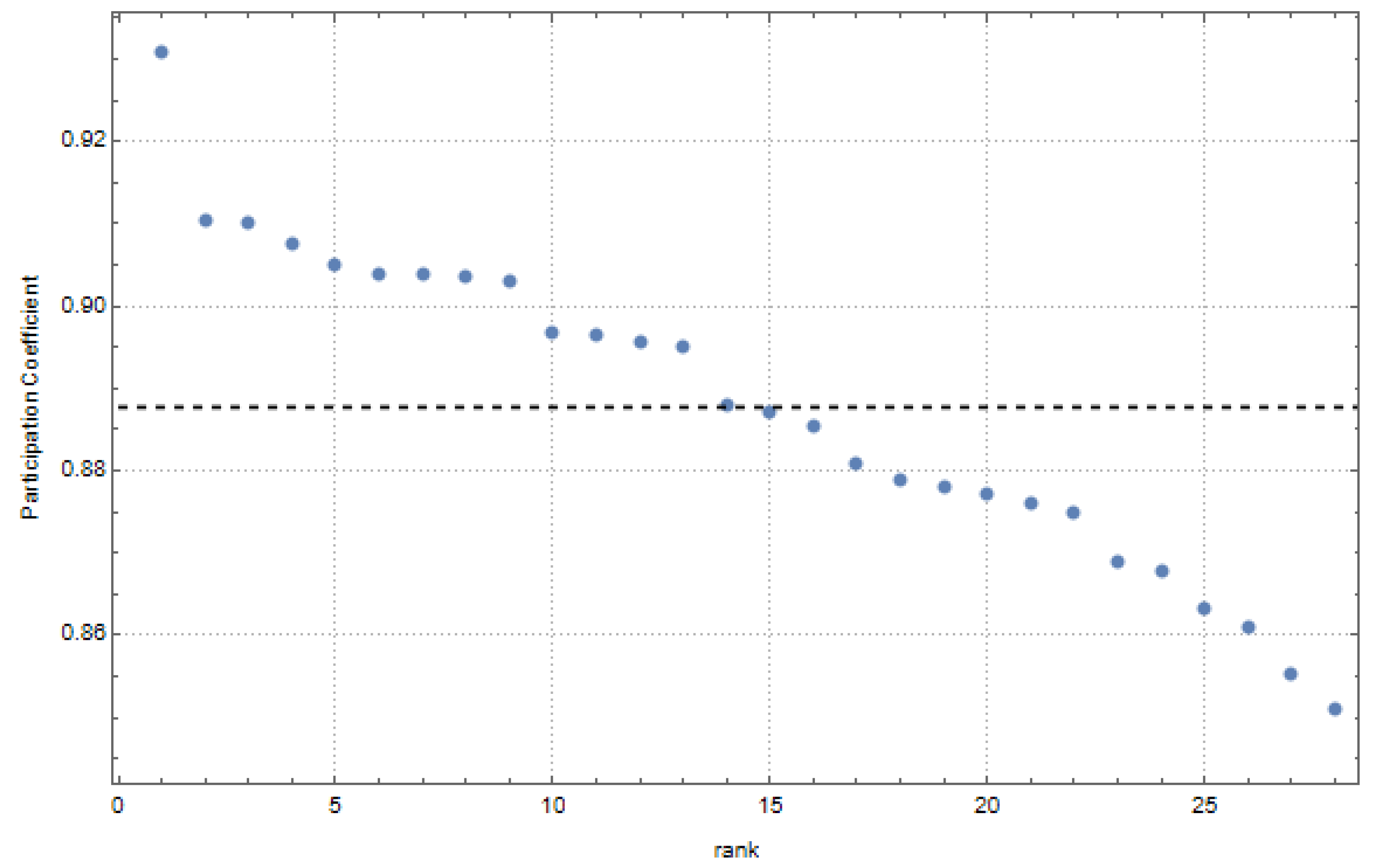
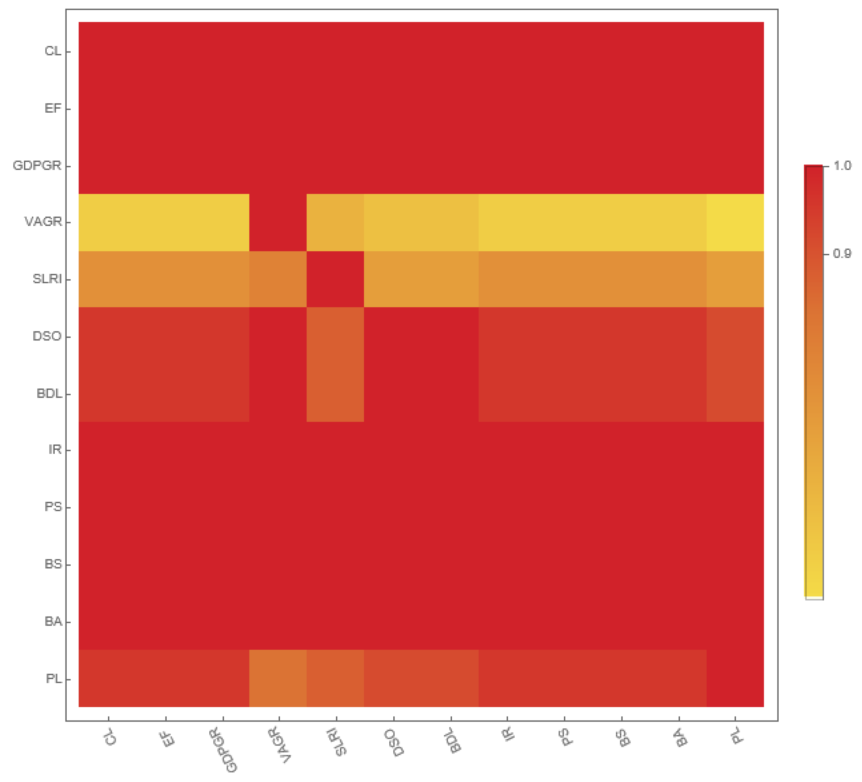
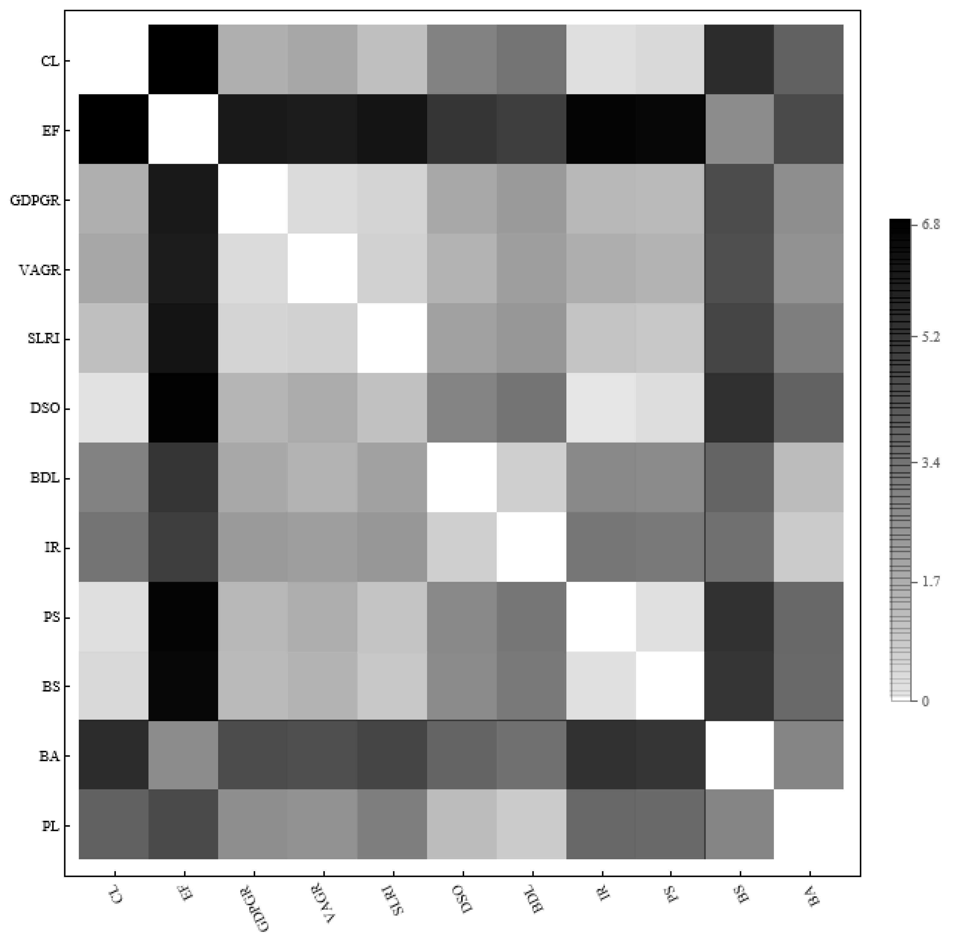
4.2. Multiplex Time Series Analysis

Data sets containing time and data can be used to hypothesize the effects of time on data and draw conclusions for future periods. Instead of assigning numerical values to different temporal states one by one, time series analysis treats data from the entire observation group as a whole and analyzes events and processes that have developed over time to shed light on the past and the future [31]. Investors can benefit from taking the right position by performing an accurate and comprehensive analysis of multivariate or univariate time series obtained from financial data. Complex network analysis is a popular type of analysis in financial data analysis. Before discussing the concepts of network and complex network, we define the concept of graph, which resembles a picture of objects and corresponding relationships.

Objects are the vertices of a graph, whereas relationships between objects are the edges of a graph. Hence, the set pair represents the graph $G=\left(V,E\right)$. In this context, $V$ is a discrete set and $E$ comprises ordered pairs of elements of $V\times V$. A network is a type of relational organization that facilitates information flow and interaction, and it is used to represent discrete data. Objects and their relationships are the most important concepts in a network. Since objects can be represented with vertices and their relationships with edges, graphs can be used to model networks. In this context, networks can be determined mathematically using the adjacency matrix [32].

The adjacency matrix of a graph with $N$ vertices is a binary matrix of type $N\times N$, with the following inputs:

$$A_{i,j}=\{\begin{array}{cc}1,& if\left(i,j\right)\in E\\ 0,& otherwise\end{array}$$

(2)

Every second, massive amounts of data are generated. Making meaningful conclusions from such data yields numerous advantages in almost every field. Hence, advances in big data collection and analysis support more comprehensive investigations. Different and more complex networks emerge as a result of these analyses. The need to transition from simple networks to complex networks has emerged, particularly in social science studies [33]. Complex networks can be used to build mathematical models and conduct econometric analyses in the field of finance. In the intricate network structure of financial markets, investor relations are quite complex, with one of the apex clusters representing investors and the other the stock market. It is challenging to identify linkages between investors in the network model, since participants only purchase and sell assets and do not physically engage with one another. The significance of complex networks in financial markets is increased by data from various historical periods where there were many investors, traded assets, and transactions [34].

We used complex network analysis to examine the connections between our variables of interest. The relationship dynamics within each country was examined through multiplex measurements.

Multiplex Measures

Consider a complex system with numerous relationships among its constituent parts. When the nature of ties can be distinguished, embedding edges in distinct layers according to their kind is an appropriate way to represent the system. Consider an $N$-node system with $M$ weighted layers. Each layer can be assigned an adjacency matrix $A^{\alpha }=\left[a_{ij}^{\alpha }\right]$, where $\alpha$ denotes the layer index. In our study, we create networks by dynamically warping multivariate time series from each region. As a result, all networks in the multiplex layers are weighted and undirected networks. Rather than degrees, we consider a node’s strength in an $\alpha$ layer as the sum of edge weights adjacent to that node. We employ $s_i^{\alpha }$ to indicate the strength of a node $i$ in the $\alpha$ layer. Furthermore, a node’s weighted edge overlapped degree $o_i$ can be defined as its total strength with $o_i={\displaystyle \sum }_{1\le \alpha \le M}{s}_i^{\alpha }$.

The strength distribution of a single-layer network is a fundamental characteristic. In multiple networks, one can examine how the strength is distributed among different nodes at each tier and across levels. In fact, nodes that serve as hubs in one layer can register a small number of connections in another layer or they can be isolated. Moreover, nodes that serve as hubs in one layer can still function as hubs in another layer.

For the purpose of this study, we used $\alpha \in \left\{CL, EQF, GDPGR, VAGR, SLRI, DSO, BDL, IR, BS, BA, PL, PS\right\}$ in order to determine the aggregated topological strength $s_i$ and the strength of the nodes in each layer $s_i^{\alpha }$. We then ordered the nodes based on their aggregated topological strength.

To better quantify correlations on node strengths, we computed the Kendall rank correlation coefficient, ${\tau }_s$, which evaluates the similarity of two ranked sequences of data $X$ and $Y$. The coefficient ${\tau }_s$ is a nonparametric measure of statistical dependency between two ranks since it makes no assumptions about the distributions of $X$ and $Y$ and accepts values ranging from −1 to 1. The following contexts are possible: if two rankings are identical, then ${\tau }_s\left(X,Y\right)=1$; if one rating is the opposite of the other, then ${\tau }_s\left(X,Y\right)=-1$; if two rankings are independent, then ${\tau }_s\left(X,Y\right)=0$. ${\tau }_s$ values obtained for the rankings of each pair of variables are depicted as a heat map in Figure 1.

As can be seen from Figure 1, when assessing the rank correlation between variables, the variable Cost of loans registered a strong negative correlation with all variables excepting Public support and GDPGR. The strongest positive correlation was set between VAD and BD.

The entropy of multiplex strength is a sensible quantity that indicates the strength distribution of node $i$ across layers. In this context, the term “entropy” can be used to describe this situation for node $i$:

$$H\left(i\right)=-{{\displaystyle \sum }}_{\alpha =1}^M\frac{s_i^{\alpha }}{o_i}ln\left(\frac{s_i^{\alpha }}{o_i}\right)$$

(3)

In the event that all linkages of a node are included in the same layer, the corresponding entropy is null. This entropy reaches its maximum if linkages are uniformly distributed across layers. The general rule is the following: when $H\left(i\right)$ is higher, the linkages of the node are uniformly distributed across layers.

Similarly, the multiplex participation coefficient $P\left(i\right)$ corresponding to node $i$ can be defined as:

$$P\left(i\right)=\frac{M}{M-1}\left(1-{\displaystyle \sum }_{\alpha =1}^M{\left(\frac{s_i^{\alpha }}{o_i}\right)}^2\right)$$

(4)

The multiplex participation coefficient assesses the weighted contribution of a node to the creation of network communities. In this sense, $P\left(i\right)$ indicates whether linkages of node $i$ are uniformly distributed across $M$ levels or whether they are concentrated in few layers. The larger $P\left(i\right)$ is, the more evenly distributed node $i$ is in the $M$ layers of the multiplex. The participation coefficient of the entire multiplex is determined by averaging $P\left(i\right)$ over all nodes. Hence, the details provided by $P\left(i\right)$ and $H\left(i\right)$ are similar.

$H\left(i\right)$ has an indeterminate form if a network includes isolated nodes. In this case, we display only the $P\left(i\right)$ distributions (Figure 2).

Figure 2 depicts the $P\left(i\right)$ distribution for the multilayer network under consideration in our study. Although the average participation coefficient of the multiplex is $0.887$, we identified the $P\left(i\right)$ distribution in the range $\left[0.8, 1\right]$, meaning the network has varied levels of node involvement in each of its 12 layers.

We further classified the multiplex nodes by the $P\left(i\right)$ and the overlapping strength of the node. The multiplex participation coefficient gives details on the distribution of incident edges across layers. The overlapping strength expresses the node’s overall importance in terms of incident edges. Starting from the multiplex participation coefficient, we can define three categories: focused nodes with $0<P\left(i\right)<\frac{1}{3}$, mixed nodes with $\frac{1}{3}\le P\left(i\right)<\frac{1}{2}$, and truly multiplex nodes with $P\left(i\right)\ge \frac{2}{3}$.

The rank distribution of the participation coefficient indicates that averages of both areas are nearly comparable. Moreover, most participation coefficients are above the value of 2/3. Consequently, it could be stated that the use of multiplex to analyze both areas is rational and beneficial. In addition, we employed the corresponding Z-score, determined as:

$$z\left(o_i\right)=\frac{o_i-{\mu }_o}{{\sigma }_o}$$

(5)

In the equation above, ${\mu }_o$ indicates the mean and ${\sigma }_o$ indicates the standard deviation corresponding to overlapping strengths. Starting from the Z-scores of the overlapping strength, hubs register a $z\left(o_i\right)\ge 0.5$, whereas ordinary nodes register a $z\left(o_i\right)<0.5$.

In this context, six categories of nodes can be identified based on the $P\left(i\right)$ and its aggregated overlapping strength $o_i$. Figure 3 illustrates this situation, with each node being represented as a point in the $\left(P_i,z\left(o_i\right)\right)$ plane.

Table 6. Multiplex participation coefficient with Z-scores.

Region	$\mathit{P}\left(\mathit{i}\right)$	$\mathit{z}\left({\mathit{o}}_{\mathit{i}}\right)$	Region	$\mathit{P}\left(\mathit{i}\right)$	$\mathit{z}\left({\mathit{o}}_{\mathit{i}}\right)$	Region	$\mathit{P}\left(\mathit{i}\right)$	$\mathit{z}\left({\mathit{o}}_{\mathit{i}}\right)$
Austria	0.9099	0.1738	Finland	0.8966	0.2161	Lithuania	0.8808	0.4079
Belgium	0.8872	−0.1165	France	0.9076	0.0770	Luxembourg	0.8950	0.5580
Bulgaria	0.8679	−0.3645	Germany	0.8966	1.6415	Malta	0.8554	0.5435
Croatia	0.8748	−0.6382	Greece	0.8759	−1.5629	Netherlands	0.9309	−0.8543
Cyprus	0.9039	−1.5439	Hungary	0.8781	−0.1266	Poland	0.9029	0.8017
Czech Republic	0.9038	0.2317	Ireland	0.8689	−1.7803	Portugal	0.8957	−0.0912
Denmark	0.9036	1.0036	Italy	0.8789	0.2159	Romania	0.8770	−2.1103
Estonia	0.9103	−0.9651	Latvia	0.8633	0.3949	Slovakia	0.8509	1.3978
Slovenia	0.8611	1.1380	Sweden	0.8853	1.6958
Spain	0.8879	0.4076	UK	0.9049	−0.7512

presents the multiplex participation coefficient $P\left(i\right)$ with corresponding Z-scores.

As indicated by Table 6, most countries (called “regions”) are multiplexes. In this sense, connections between these countries are rather strong. However, only nations such as Denmark, Germany, Sweden, Slovakia, and Slovenia reported strong hub nodes in this topology. In other words, these countries serve as cluster forerunners. Moreover, although Luxembourg, Malta, and Poland can be considered hubs, they registered values close to the boundary. In addition, most Western European countries manifest the tendency of being a hub in the multiplex setting.

We further quantified the relevance of each layer. Given the presence of an edge linking identical nodes within a layer, the conditional probability of detecting a connection at a layer can be defined as:

$$\mathbb{P}\left(a_{ij}|{a^{\prime }}_{ij}\right)=\frac{{{\displaystyle \sum }}_{ij}{a}_{ij}{a^{\prime }}_{ij}}{{{\displaystyle \sum }}_{ij}{a}_{ij}}$$

(6)

Figure 4 depicts the conditional probability as a heat map.

Each row in the heat map indicates the probability that edges from one layer be included in other layers. Among our variables, VAGR and SLRI displayed sparsity regarding probability. We can state that such variables are less beneficial. Therefore, the existence of edges and their connection strength become critical aspects.

We compared the Wasserstaien-1 distances between the distributions of node strength from each dominant layer to establish which layers registered the largest node-strength similarity.

Figure 5 shows the results of this comparison.

From Figure 5, we can infer that the least similar distributions emerged between the EF and BA layers. Moreover, the GDPGR and SLRI layers were useful in forming multi-regional correlations. In addition, it can be observed that various clusters occurred from the distance matrix. For example, GDPGR, VAGR, and SLRI displayed the tendency of forming clusters among themselves. However, taking into account conditional possibilities, the variable GDPGR was expected to serve as the forerunner of this cluster.

5. Discussion

Our research study investigated relevant determinants of economic growth for small and medium enterprises across the 28 countries belonging to the European Union for a period of 16 years, namely 2005–2020. Our methodological approach comprised two relevant methods: panel first-difference generalized method of moments (GMM) and multiplex time series analysis.

The panel first-difference generalized method of moments revealed important results. In the first place, Cost of loans was mainly influenced by Interest rate. Hence, when the latter decreases, smaller loans become more costly because credit institutions are incentivized to grant large loans for profit concerns. As expected, in terms of Equity fund, the largest positive impact was played by Business angels, who are generally very open and inclined to support new business endeavors across Europe. A similar role was played by Private lenders, who also are risk-takers in the business realm. Third, across European markets, Business angels were the ones boosting GDP growth rate with their willingness to finance new and innovative activities. Fourth, Value added growth rate was significantly shaped by the variables Bank support and Business angels.

Our study also examined the dynamics of this continuity using multiplex time series analysis, which layered many factors related to SME activities in the European Union. Although our approach regarded countries as multiplex nodes within the demographic structure, country collaborations were measured via time series similarities for all variables in each layer.

The multiplex analysis results indicated that countries in the European Union cooperated with each other—namely, all nodes were truly multiplex from a mathematical standpoint. Hence, we observed that SMEs from Denmark, Germany, Sweden, Slovakia, and Slovenia seemed to work in conjunction with other countries for all layer variables. The countries where this trend was registered the least were Cyprus, Greece, Ireland, and Romania. Other countries displayed the tendency of intensifying cooperation—in other words, of becoming hub nodes. Collaborations that took place in the context of value added growth rate were not registered in other layers. A similar tendency was also observed for the variables Strength of legal rights index, Public support, Days sales outstanding, and Bad debt loss.

The Wasserstein distance matrix revealed that the layers comprising Equity fund and Business angels led to the least similar distributions. Furthermore, Gross domestic product growth rate and Strength of legal rights index supported multi-regional connections. Additionally, the distance matrix included numerous clusters. For instance, the variables Gross domestic product growth rate, Value added growth rate, and Strength of legal rights index were frequently grouped together, mainly due to the first variable.

6. Conclusions

As reported by official statistics [35] and empirical research on economic markets [36], small and medium enterprises are considered the backbone of global economy, irrespective of the level of country development. Moreover, small and medium enterprises possess real innovative capabilities that can boost their advancement in both young and mature markets. In this context, our research provides answers that could assist national and regional authorities in boosting economic growth by stimulating business activities of small and medium enterprises.

Cooperation among economic players such as SMEs can be challenging since any free rider within a cooperative economic group can reap the benefits of others’ cooperation at no cost. Nevertheless, the propensity of SMEs to cooperate with other actors who share their demographic and structural characteristics supports the market economy. Additionally, it is believed that reciprocity yields cooperation. Hence, SME networks, whether physically accessible or not, may encourage continuity in SMEs’ collaborative processes and development.

In our view, since SMEs are vital for the regional economy, the European Union should increase its support toward these categories of economic entities by granting funds that can be used to partially pay for their employees’ salaries and contributions. This would also benefit the labor market by increasing the number of employees (thus integrating especially those recently graduated from college or older adults) and would support SMEs’ access to the European market.

In addition, governments can also assist SME activities by enacting taxpaying facilities, tax mitigation, or tax exemptions, especially in strategic sectors within national economies (e.g., agriculture, hospitality, tourism).

Last but not least, support for SMEs should come from banks, which can offer credit facilities, interest rate caps, or loans under favorable conditions. In the period 2008–2019, the cumbersome formalities of some banks in granting loans, especially for working capital, contributed to the rejection of many applications from SMEs regarding potential bank loans.

In conclusion, considerable mitigations of loan costs can be achieved by reducing interest rates, commissions, bank fees, and the number of days in which invoices issued by SMEs are paid. Moreover, local authorities are gradually inclined to support SMEs by directly awarding them infrastructure projects or by purchasing goods and services that are necessary within public institutions. At the same time, authorities can materialize this support for SMEs under the form of accessible financing, which can provide a sustainable level of economic growth in the years to come.

As with any research study, our investigation has certain limitations. In the first place, the study focused on 28 countries from Europe. Future research might consider examining how the financing of small and medium enterprises influences economic growth on countries from other continents. In the second place, the analyzed period spanned 16 years. Other studies might consider expanding the time frame by including several decades while considering major economic downturns. In the third place, the independent variable set could be widened by including factors such as leasing, supply chain financing, or trade credit.

Our research study emphasizes that new projects advanced by small and medium enterprises may benefit from the support of business angels and other similar investors that understand the importance of incentivizing entrepreneurial initiatives across the European Union. In addition, given that the latest advances in financial technology have been regarded as major drivers of sustainable economic growth [37,38,39], future research directions could focus on how this technology may facilitate the access of small and medium enterprises to numerous business opportunities.

References

1. Bammer, G.; Smithson, M. Uncertainty and Risk: Multidisciplinary Perspectives, 1st ed.; Routledge: Oxon, UK, 2009. [Google Scholar]
2. Biello, D. Can Math Beat Financial Markets? Scientific American. 2011. Available online: https://www.scientificamerican.com/article/can-math-beat-financial-markets/ (accessed on 12 August 2022).
3. Heyman, B. Risk and uncertainty: A review of three recent texts. Health Risk Soc. 2009, 11, 87–90. [Google Scholar] [CrossRef]
4. Kirikkaleli, D. Does political risk matter for economic and financial risks in Venezuela? J. Econ. Struct. 2020, 9, 3. [Google Scholar] [CrossRef] [Green Version]
5. Ben Ghozzi, B.; Chaibi, H. Political risks and financial markets: Emerging vs. developed economies. EuroMed J. Bus. 2021. [Google Scholar] [CrossRef]
6. Beckert, J. The social order of markets. Theory Soc. 2009, 38, 245–269. [Google Scholar] [CrossRef] [Green Version]
7. European Commission. User Guide to the SME Definition; Publications Office of the European Union: Luxembourg, 2017. Available online: https://ec.europa.eu/regional_policy/sources/conferences/state-aid/sme/smedefinitionguide_en.pdf (accessed on 12 August 2022).
8. Small and Medium Enterprises (SMEs) Finance. Available online: https://www.worldbank.org/en/topic/smefinance (accessed on 12 October 2021).
9. International Labour Organization. Small Matters: Global Evidence on the Contribution to Employment by the Self-employed, Micro-Enterprises and SMEs; International Labour Organization: Geneva, Switzerland, 2019. [Google Scholar]
10. OECD. Enhancing the Contributions of SMEs in a Global and Digitalised Economy. Available online: https://www.oecd.org/industry/C-MIN-2017-8-EN.pdf (accessed on 14 August 2022).
11. Lin, D.-Y.; Rayavarapu, S.N.; Tadjeddine, K.; Yeoh, R. Beyond Financials: Helping Small and Medium-Size Enterprises Thrive. Available online: https://www.mckinsey.com/industries/public-and-social-sector/our-insights/beyond-financials-helping-small-and-medium-size-enterprises-thrive (accessed on 14 August 2022).
12. Batrancea, L.M. Determinants of economic growth across the European Union: A panel data analysis on small and medium enterprises. Sustainability 2022, 14, 4797. [Google Scholar] [CrossRef]
13. Maow, B.A. The impact of small and medium enterprises (SMEs) on economic growth and job creation in Somalia. J. Econ. Policy Res. 2021, 8, 45–56. [Google Scholar]
14. OECD. Small Businesses, Job Creation and Growth: Facts, Obstacles and Best Practices. Available online: https://www.oecd.org/cfe/smes/2090740.pdf (accessed on 15 August 2022).
15. Cooney, T.M. Entrepreneurial Skills for Growth-oriented Businesses. In Proceedings of the Skills Development for SMEs and Entrepreneurship, Copenhagen, Denmark, 28 November 2012; Available online: https://www.oecd.org/cfe/leed/Cooney_entrepreneurship_skills_HGF.pdf (accessed on 12 August 2022).
16. OECD. SMEs, Entrepreneurship and Innovation; OECD: Paris, France, 2010. Available online: https://read.oecd-ilibrary.org/industry-and-services/smes-entrepreneurship-and-innovation_9789264080355-en#page1 (accessed on 12 August 2022).
17. OECD. New Approaches to SME and Entrepreneurship Financing: Broadening the Range of Instruments. Available online: https://www.oecd.org/cfe/smes/New-Approaches-SME-full-report.pdf (accessed on 13 August 2022).
18. Clifford, C. Billionaire Richard Branson: This Simple Trick Is the Best Way to Come up with an Idea for a Successful Business. Available online: https://www.cnbc.com/2018/01/03/richard-branson-how-to-come-up-with-a-successful-business-idea.html (accessed on 12 August 2022).
19. Yoshino, N.; Taghizadeh-Hesary, F. The Role of SMEs in Asia and Their Difficulties in Accessing Finance; ADBI Working Paper 911; Asian Development Bank Institute: Tokyo, Japan, 2018; Available online: https://www.adb.org/publications/role-smes-asia-and-their-difficulties-accessing-finance (accessed on 13 August 2022).
20. Hossain, M.; Yoshino, N.; Taghizadeh-Hesary, F. Optimal branching strategy, local financial development, and SMEs’ performance. Econ. Model. 2021, 96, 421–432. [Google Scholar] [CrossRef]
21. Kapitsinis, N.; Munday, M.; Roberts, A. Exploring a low SME equity equilibrium in Wales. Eur. Plan. Stud. 2021, 10, 1777–1797. [Google Scholar] [CrossRef]
22. Nigohosyan, D.; Vutsova, A.; Vassileva, I. Effectiveness and efficiency of the EU-supported energy efficiency measures for SMEs in Bulgaria in the period 2014–2020: Programme design implications. Energy Effic. 2021, 14, 24. [Google Scholar] [CrossRef]
23. Hasan, I.; Jackowicz, K.; Jagiello, R.; Kowalewski, O.; Kozlowski, L. Local banks as difficult-to-replace SME lenders: Evidence from bank corrective programs. J. Bank. Financ. 2021, 123, 106029. [Google Scholar] [CrossRef]
24. Mkhaiber, A.; Werner, R.A. The relationship between bank size and the propensity to lend to small firms: New empirical evidence from a large sample. J. Int. Money Financ. 2021, 110, 102281. [Google Scholar] [CrossRef]
25. Ciampi, F.; Giannozzi, A.; Marzi, G.; Altman, E.I. Rethinking SME default prediction: A systematic literature review and future perspectives. Scientometrics 2021, 126, 2141–2188. [Google Scholar] [CrossRef] [PubMed]
26. Eldridge, D.; Nisar, T.M.; Torchia, M. What impact does equity crowdfunding have on SME innovation and growth? An empirical study. Small Bus. Econ. 2021, 56, 105–120. [Google Scholar] [CrossRef] [Green Version]
27. Mina, A.; Di Minin, A.; Martelli, I.; Testa, G.; Santoleri, P. Public funding of innovation: Exploring applications and allocations of the European SME Instrument. Res. Policy 2021, 50, 104131. [Google Scholar] [CrossRef]
28. Kim, H.S.; Cho, K.S. Financing resources of SMEs and firm performance: Evidence from Korea. Asian J. Bus. Account. 2020, 13, 1–26. [Google Scholar] [CrossRef]
29. Wang, X.D.; Han, L.; Huang, X.; Mi, B. The financial and operational impacts of European SMEs’ use of trade credit as a substitute for bank credit. Eur. J. Financ. 2021, 27, 796–825. [Google Scholar] [CrossRef]
30. Eurostat Database. Available online: https://ec.europa.eu/eurostat (accessed on 12 August 2022).
31. Lacasa, L.; Nicosia, V.; Latora, V. Network structure of multivariate time series. Sci. Rep. 2015, 5, 15508. [Google Scholar] [CrossRef] [PubMed] [Green Version]
32. Newman, M.E.J. Networks: An Introduction; Oxford University Press: Oxford, MS, USA, 2010. [Google Scholar]
33. Albert, R.; Barabási, A.-L. Statistical mechanisms of complex networks. Rev. Mod. Phys. 2002, 74, 47. [Google Scholar] [CrossRef] [Green Version]
34. D′Arcangelis, A.M.; Rotundo, G. Complex networks in finance. In Complex Networks and Dynamics; Commendatore, P., Matilla-García, M., Varela, L.M., Cánovas, J.S., Eds.; Springer: Cham, Switzerland, 2016; pp. 209–235. [Google Scholar]
35. OECD. Financing SMEs and Entrepreneurs 2022; OECD: Paris, France, 2022. Available online: https://www.oecd.org/cfe/smes/financing-smes-and-entrepreneurs-23065265.htm (accessed on 14 August 2022).
36. Batrancea, L.; Rathnaswamy, M.M.; Batrancea, I.; Nichita, A.; Rus, M.-I.; Tulai, H.; Fatacean, G.; Masca, E.S.; Morar, I.D. Adjusted net savings of CEE and Baltic nations in the context of sustainable economic growth: A panel data analysis. J. Risk Financ. Manag. 2020, 13, 234. [Google Scholar]
37. Deng, X.; Huang, Z.; Cheng, X. FinTech and sustainable development: Evidence from China based on P2P data. Sustainability 2019, 11, 6434. [Google Scholar] [CrossRef]
38. Leong, K.; Sung, A.; Teissier, C. Financial technology for sustainable development. In Partnership for the Goals; Leal Filho, W., Marisa Azul, A., Brandli, L., Lange Salvia, A., Wall, T., Eds.; Springer: Cham, Switzerland, 2021; pp. 453–466. [Google Scholar]
39. Cen, T.; He, R. Fintech, Green Finance and Sustainable Development. In Proceedings of the 2018 International Conference on Management, Economics, Education, Arts and Humanities (MEEAH 2018); Atlantis Press: Amsterdam, The Netherlands, 2018; pp. 222–225. [Google Scholar]
Figure 1. Kendall correlation coefficient of variables.
Sustainability 14 15318 g001
Figure 2. Rank distribution of participation coefficients. Note: The dashed horizontal line represents the average participation coefficient.
Sustainability 14 15318 g002
Figure 3. Map of the responsibilities of nodes in a multilayer network. Note: Although two nodes may have identical Z-scores, their functions might change significantly due to the value of the multiplex participation coefficient.
Sustainability 14 15318 g003
Figure 4. Heat map of conditional probabilities of links within each layer.
Sustainability 14 15318 g004
Figure 5. Wasserstein distance matrix of dominant layers.
Sustainability 14 15318 g005