Abstract
The average hourly income of taxi drivers could be improved by understanding the realized income of taxi drivers and investigating the variables that determine their income. Based on 4.85 million taxi-trajectory GPS records in Shenzhen, China, this study built a multi-layer road index system in order to reveal the behavioral patterns of drivers with varying income levels. On this basis, late-shift drivers were further selected and classified into two categories, namely high-earning and low-earning groups. Each driver within these groups was further classified into three income levels and four categories of factors were defined (i.e., occupied trips and duration, operational region, search speed, and taxi service strategies). The sample-based multinomial logit model was used to reveal the significance of these income-influencing factors. The results indicate significant differences in the drivers’ behavioral habits and experience. For instance, high-earning drivers focused more on improving efficiency using mobility intelligence, while low-earning drivers were more likely to invest in working hours to boost their revenue.
1. Introduction
Taxis are an important source of transportation due to their adaptability and wide coverage across time and space. The mobile sensing device produces a massive volume of electronic footprints (e.g., cellphones and GPS navigators), which gives us a unique insight into understanding human behavior and crowd intelligence [1]. The GPS system of the taxi transmits the real-time information, periodically, to a server, including taxi ID, latitude and longitude, time stamp, instantaneous speed, direction angle, and if passengers are onboard [2,3,4]. These data have been widely used in investigating the wisdom and experience of taxi drivers [2,5]. At present, the mining of taxi trajectories is still a hot topic for path recommendation [5,6,7], mobility pattern detection [3,8], and congestion estimation [9,10], in improving the experiences of taxi drivers.
High-performing taxi drivers are likely to aim to maximize profits by minimizing their expenses [11]. As a result, nonstandard taxi activities [2], such as passenger denial [4,12], unmitering [13], and detouring [3,14], have increased. These improper driving behaviors are commonly observed in Shenzhen, China. Since 2004, nearly 200 taxi strikes have taken place across China, involving more than 100 cities. The survey claims that drivers refuse to serve because they believe their income is lower than they deserve, and they are unsure of how to increase it. Therefore, the study on raising drivers’ income would not only help drivers, but also increase the availability of taxi services and better meet clients’ travel needs. Consequently, studies on how to improve the income of taxi drivers will benefit multiple objects (e.g., drivers, passengers, management businesses).
Previous research has looked at the variable factors in influencing the taxi business. GPS patterns have been used to underline these factors, which include personal driving models [15], pickup likelihood [16], working hours [17], changes in driving speed [1,15], and taxi service strategy, etc. For instance, the space-time patterns on cruise journeys and stopping points [18], hot-spot regions [19], mileage or time utilization ratios [20], and region selection [1,21,22] are some of the key components of taxi service strategy, which impact the crowd intelligence of taxi drivers. Some studies have included ticket prices [17,23], supply-demand ratios of the taxi market [24], weather variables [25] etc., to further assess their influence on drivers’ income. Although these elements are linked to the behavior of taxi drivers, our knowledge of the causes of low income due to driver expectations is still insufficient.
In addition, the research demonstrates significant differences between the driving behavior of various income levels, including the cruising time, cruising frequency, and stopping sites [26]. Taxi drivers are using a variety of techniques to select driving regions in finding customers. Therefore, the weekly income of a driver is relatively stable [21]. Yuan divided taxi drivers into three groups based on the distance charged (occupied) per unit of working time. The main points of income disparity for a taxi driver are where he/she may swiftly pick up a customer and the average travelling distance [27]. It has been demonstrated that experienced and self-improving drivers increase their earning efficiency and maintain their behavioral habits over time [28]. Consequently, the drivers’ behavior patterns during pick-up and passenger-seeking sequences influence the differences in their income levels, depending on the duration of the work, and will remain consistent over time.
Therefore, we take the realized average hourly income as a standard in dividing the drivers into two groups, namely the high-earning group (higher than the average realized income) and the low-earning group (lower than the average realized income). Each group was further classified into three levels, namely high, middle, and low income (0–20, 40–60, and 80–100 percentiles of income in ascending order). Map matching and multi-layer road-index (MRI) systems were established based on taxi trace data. With the MRI system, we identified factors relating to four aspects of occupied trips and duration, region preference, speed, and taxi service strategies. A selected sample-based multinomial logit (SML) model was used to correlate income level with the factors and determine their significance within the two groups. Finally, we clarified the contributions of each factor on the different income levels in different groups.
2. Preliminaries
2.1. MRI System and Map Data
The construction of a data aggregation unit is the foundation of spatial statistics analysis. With this unit, dispersed trip samples and local characteristics can be partitioned uniformly and countably within a large-scale traffic network. To avoid the mix-up of different road-segments, we did not follow the traditional grid or traffic analysis zones (TAZs) approaching in delineating the study area. Instead, an MRI system [29] is used by extending a road-indexing method called “intersection continuity negotiation” [30,31]. The map (we used in this study is the Shenzhen Transportation Planning Network, see Figure 1) is equipped with the MRI system consisting of 2476 road units (RUs), derived from 21,115 map links, which will highly improve the calculation efficiency of the data mining process [29].
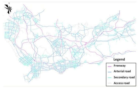
Figure 1.
GIS data of the City of Shenzhen.
2.2. Taxi Trace Data
The taxi trace data we used were retrieved from the City of Shenzhen Taxi database [32], spanning a week, from 15 January to 21 January 2015. The data set contained approximately 194 million occupied GPS points, derived from 15,726 taxis. For convenience, all trace points were divided into 4.85 million trips with customers. Each trip had time-series records of latitude, longitude, and time stamps, with an average sampling rate of around 30 s.
In order to distinguish between early- and late-shift drivers, the driver operating indicators, namely the number of hired taxis and the ratio of vacant/total time (RVTT), are chosen to calculate the driver’s handover time. Figure 2 demonstrates that the number of hired taxis began to quickly fall after midnight and stabilized between 07:00 and 08:00. During 00:00–08:00, the RVTT increased before decreasing, reaching a turning point at 07:00. Therefore, 06:00–07:00 was chosen as the early handover window. After 08:00, the number of hired taxis appears to stabilize to approximately 8300, indicating that the number of hired taxis is more consistent during the day than at night. As the RVTT was at its height between 18:00 and 19:00, 18:00 to 19:00 was chosen as the late handover period. On their handover journey, it is common knowledge that drivers will abandon passengers whose destinations do not match the direction of the handover point. Through our analysis of the taxi market, we determined that the typical late handover time is between 17:00 and 19:00. Consequently, based on the above data analysis, we hypothesized that the operating hours of early-shift drivers are 07:00 to 19:00 and those of late-shift drivers are 19:00 to 07:00. This offers a foundation for late-driver classification data processing.

Figure 2.
Trend of the ratio of RVTT(ratio of vacant/total time).
2.3. Calculation of Income
Using the MRI technology and taxi trace data, we determined the income of each driver on each route. Figure 3 shows that the Guan Nei and Guan Wai districts in Shenzhen have different taxi charging standards.
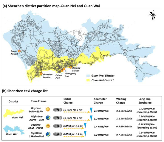
Figure 3.
Shenzhen district partition and taxi charge list.
3. Method
GPS trajectories of over 10,000 taxis in Shenzhen were studied by MRI with a given map. taxi drivers were categorized to identify the potential income-affecting factors. The SML model was developed to interpret the significant factors influencing income.
3.1. Categorizing Taxi Drivers by Income Level
It was important to categorize drivers into early-shift and late-shift drivers in order to identify their performance. As night-shift drivers are a more accurate representation of the population, nighttime driving methods are less influenced by road conditions. As vehicles from Guan Wai cannot enter Guan Nei to solicit passengers, we only selected night-shift drivers in the Guan Nei district for analysis. In addition, we excluded samples with an abnormal performance, such as those with a daily night-shift income <200 yuan or >1200 yuan, as well as samples with a daily work time <4 h. The remaining sample size was 8038. The income between 19:00 and 07:00 displays a Gaussian distribution with a mean of 529.29 yuan and a standard deviation of 102.80 yuan, as depicted in Figure 4.

Figure 4.
Distribution of average night drivers’ income.
In order to draw a convincing conclusion, it is essential to locate drivers with a consistent performance. A suitable degree of sample selection can increase the accuracy of model predictions and better identify the primary factors influencing the income of truck drivers [15,24]. Therefore, drivers with a standard deviation ranking within 50% were selected [24], as shown in Figure 5. In addition, low-, medium-, and high-income levels were classified according to the 0–20, 40–60, and 80–100 percentiles (Y = 1, 2, and 3, respectively, for low, medium, and high-income levels). Average night-shift drivers’ incomes at the 20, 40, 60, and 80 percentiles are 437.46, 455.59, 552.12, and 608.37 yuan, respectively. More than 4000 cab drivers were removed as the final sample and divided into low-, medium-, and high-income levels (accounting for 15%, 18%, and 18%, respectively).
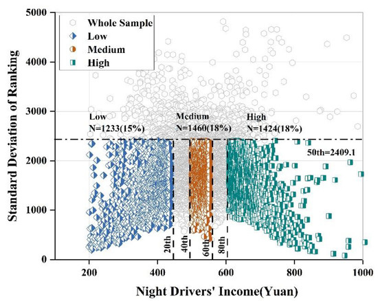
Figure 5.
Sample selection and categorization of drivers.
Drivers with low-, medium-, and high-income levels were further studied as high- and low-earning groups, which is more conducive to investigating the important elements impacting income, because Taxi drivers with a realized income represent various driver behavior [33]. Realized income (yuan/h) was obtained through working hours. The predicted income (yuan/h) was computed as the average income of the group. Drivers who earned more than the group’s average income were classed as high-earning, while those who earned less were classified as low-earning.
Additionally, the realized income followed a Gaussian distribution, with a mean of 72.31 yuan and a standard deviation of 12.07 yuan, as shown in Figure 6. The estimated incomes for those with low-, medium-, and high-incomes are 66.41, 71.09, and 80.08 yuan. The sample sizes of the high- and low-expectation groups were 1968 and 2148. Furthermore, 34%, 27%, and 29% of the samples in the high-expectation group represented high-, medium-, and low-income. The sample sizes of high-, medium-, and low-income in the low-expectation group accounted for 26%, 34%, and 40%.

Figure 6.
Distribution of average realized income.
3.2. Defining Correlated Variables Affecting Income Level
Variables, including duration and distance, region of operation, passenger flow, and travel speed, etc., have been analyzed in order to indicate their impact on drivers’ earnings. In addition, in this research, we focused on service delivery methodologies to determine the income-affecting elements [2,34].
3.2.1. Occupied Trips and Duration
Occupied trips and duration [17] are undoubtedly the most important factors for determining the level of income. Duration includes occupied time, vacant time, and stop time in the driver’s operation. In addition, to account for the consistency of the driver’s performance, we calculated the standard deviation of the indicators using weekly data and added them into the influencing factors.
Definition 1
(Standard deviation of occupied trips). For a given taxi driver, the value of occupied trips refers to the average number of daily passenger delivery trips in a week. The total number of trips is composed of the number of occupied trips and the number of passenger-searching trips. The standard deviation of occupied trips indicates the degree of dispersion of the one-week data of occupied trips. This can be calculated as follows:
where is the number of occupied trips on day
of a week;
is the mean number of occupied trips in a week.
Definition 2
(Standard deviation of occupied time). For a given taxi driver, occupied time is the average daily time that the taxi is occupied by customers in a week. The driver’s work time consists of occupied time, vacant time, and stop time. The standard deviation of occupied time indicates the degree of dispersion of the one-week data of occupied time. It can be calculated as follows:
where is the occupied time on day of a week; is the mean value of occupied time in a week.
Definition 3
(Standard deviation of vacant time). For a given taxi driver, vacant time is the average daily time spent vacant while searching for the next customer in a week. The standard deviation of vacant time indicates the degree of dispersion of the one-week data of vacant time. It can be calculated as follows:
where is the vacant time on day of a week; is the mean value of vacant time in a week.
3.2.2. Operational Region
Drivers with varying levels of income have varying preferences for operating sites [22,35]. This is because the operational region impacts ridership and taxi charge norms (as shown in Figure 3), both of which impact profitability. Observing the travel trajectory of drivers revealed that they prefer a specific operational zone.
Definition 4
(Search-path preference). Search-path preference was calculated according to the proportion of search distance in Guan Nei district as follows:
where indicates the distance when searching for customers in Guan Nei district; indicates the total distance when searching for customers.
3.2.3. Search Speed
Speed is a significant measure of a driver’s experience and work productivity. In this research, we classified the speed into two categories, namely, the speed after the customer gets into the taxi and the speed on arbitrary routes while searching for customers.
According to Qin, the delivery speed is significantly positively correlated with income [24]. In this research, we primarily analyzed the effect of driver search speed on income.
Definition 5
(Search speed). For a given driver, search speed (m/s) is the average speed for all trips, from vehicle vacancy to finding the next passenger; it is denoted as SES. Travel speed is the ratio of each search distance to travel time, which is obtained by referring to the dynamics of the GPS trajectory.
3.2.4. Driver Service Strategies
Expert operating strategies can increase a driver’s earnings in the era of ride hailing [36]. Previous studies of drivers’ service strategies have focused on passenger-search strategies, passenger-delivery strategies, and service-region preferences [1]. There are two aims for passenger-search: maximizing profit and maximizing demand coverage [27]. Choosing similar spatiotemporal areas and dropping off customers as quickly as possible can also increase profits. Previous research [21] utilized service-strategy measures such as occupied distance, occupied duration, and capacity usage, but they are insufficiently detailed. The following defines drivers’ service strategies from the perspective of time and space.
Definition 6
(Ratio of long-distance service). Ten kilometers is taken as the threshold of long-distance service. The ratio of long-distance service refers to the ratio of the number of occupied trips longer than 10 km to the total number of occupied trips:
where denotes the daily follow distance, which is the distance after subtracting the initial distance from the total distance (initial distance value is 2 km in Guan Nei district). For a long-distance service of 10 km, the follow distance is 8 km. denotes the number of daily passenger delivery trips, except within the distance of the starting price.
Definition 7
(Search-distance ratio). The search-distance ratio refers to the proportion of distance drivers spend searching for customers:
where indicates the total distance in the delivery process.
Definition 8
(Ratio of noninitial charge trips). The ratio of noninitial charge trips refers to the proportion of in occupied trips:
where indicates occupied trips.
Definition 9
(Occupied-time ratio). Occupied-time ratio refers to the proportion of time drivers spend occupied in daily work time:
where indicates the work time and indicates occupied time.
3.3. Discretized Factors
Before model fitting, all associated variables were discretized. The impact factors were found to be continuous among taxi drivers whose standard deviations ranked within 50% (Figure 7, Figure 8 and Figure 9). The distribution is violin-shaped, with a central concentration and sparseness on both sides. Therefore, each variable was divided into three homogenous sets of dummy variables. The corresponding number for each factor is 1, 2, and 3, in parallel with the drivers in the 0–20, 21–80, or 81–100 percentile.

Figure 7.
Violin plot of and .

Figure 8.
Violin plot of , , and .

Figure 9.
Violin plot of , and .
3.4. Applying a Selected Sample-Based Multinomial Logit (SML) Model
Due to its great mathematical and statistical explanatory ability, the Multiple Indicator Logit (ML) model [37] has been widely used, particularly for conducting multiple scenario analyses from a practical statistical standpoint. Normally, the dependent variables should initially be regarded as multiclass variables corresponding to different levels. In addition, stratified sample selection was deemed more useful for identifying the most influential factors on income. We chose the top, middle, and bottom 20% of drivers. Based on the average realized income, high- and low-earning groups were categorized.
The utilities of various income levels are not identical, and taxi drivers will be predisposed to a particular income level. For the purposes of this study, taxi drivers were defined as those who can freely determine their work hours and perceive enough route options for a given origin–destination pair. Drivers must anticipate how much they will earn per hour if they continue working after each trip, as their earnings are not based on known wage rates but, rather, on random chance.
The likelihood of a specific income level can be calculated by the statistical model based on these three classifications of driver types. The probability of driver ’s income level is calculated as (9):
where is the income level of driver , is the probability of driver in the income level , is the utility function of driver in income level . Provided there is a linear relationship between and given a set of factors .
where is a vector of the potential explanatory variables, including occupied trips and duration, operational region, delivery and search speed, and driver service strategies; is the reference group, and is the effect coefficient of the corresponding variable. is an error term that accounts for unobserved factors influencing income level and is assumed to be identically and independently distributed.
An estimable severity model can be derived by assuming a generalized extreme value (GEV) distributional form for the error term. Based on the above, the income for night-shift taxi drivers was established by using the following equation:
where is the total number of income levels, is the set of income level .
4. Results and Discussion
The factors (in Section 3.2) were put into formula (10) as the variable , according to the different income levels of the high-earning and low-earning groups ( = 1, 2, and 3 for low-, medium-, and high-income levels, respectively). There are nine variables, meaning = 9. The covariance between the variables is confirmed by the data analysis software (see Section 4.1). is the effect coefficient of the corresponding variable. The values of and the overall performance of the model are shown in Section 4.2. Equation (11) represents the probability of the driver’s income level. Due to the large number of parameters, the formulae will not be listed in the later part of this article. The Odds ratio of the statistical indicator will be used to analyze the influencing degree of variables on the income level.
4.1. Collinearity Diagnosis of the Factors
Collinearity refers to an issue which impacts the accuracy of model fitting. As the most common measure of a collinearity test, the variance inflation factors (VIF) were calculated before fitting the SML model. A normal VIF value is no less than 1. The larger the VIF, the greater the collinearity in the current factors. In practice, a VIF exceeding 4 indicates that the corresponding independent variables need further consideration. A VIF greater than 10 indicates serious collinearity, and some form of adjustment must be made. Table 1 shows the details of the check for collinearity. For each factor, all VIFs ranged between 1.0 and 2.2, which is significantly below 4; that is, there was no significant collinearity between the nine factors. Therefore, all factors could be input into the SML model.

Table 1.
Collinearity detection of factors affecting income.
4.2. SML Model Results and Significant Factors
Table 2 shows the performance of two SML models. For each model, the p-value is less than 0.05, which means that at least one input factor was detected with a significant dominance ratio (OR). In addition, the pseudo R2 values indicate the extent to which the variation in the dependent variable can be explained by the input factors. Pseudo-R2 was below 0.5, but within the relatively normal range; both models still had some explanatory power.
Table 2.
Overall model performance statistics.
Table 3 shows the results of the SML model constructed with high- and low-earning drivers. The results show that driver service-strategy indicators had an important effect on income for both high- and low-earning drivers. However, the role of service strategies was different for the two types of taxi drivers. Specifically, the common factors affecting drivers’ income were , , , , and . It is worth noting that is an important factor that affects income among high-earning drivers (positive odd ratio (OR) of = 4.29, 1.35; positive odd ratio (OR) of = 1.93, 1.55). A driver’s accurate judgment of passenger flow is an important aspect of their experience. A more experienced driver will have a greater likelihood of a higher-than-average expected income. Another distinguishing factor that affects the income of high-earning drivers is . The relationship between and income in high-earning drivers is negatively correlated (negative odd ratio (OR) of = 0.18, 0.89; positive odd ratio (OR) of = 0.18, 0.89). Ending a trip within a short distance is conducive to increasing income and increasing the cost of revenue per unit time. This has higher requirements for drivers in the selection of locations for short-distance passengers to board the vehicle.
Table 3.
SML model results.
In contrast to high-earning drivers, and have a greater effect on the income of low-earning drivers. For example, the negative OR of is 0.48 and 0.46 of the low-income and high-income drivers, respectively; the negative OR of is 0.66, 0.62 of the middle-income drivers and high-income drivers, respectively; The positive OR of is 9.33, 2.66 of the low-income drivers and high-income drivers, respectively; the positive OR of is 5.95, 3.65 of the middle-income drivers and high-income drivers, respectively. This means that, among drivers with low-income expectations, vacant time and occupied time are prone to fluctuation. This is associated with a low expected income, and it is inevitable that there is a possibility of being inactive at work. In short, high-earning drivers have mobility intelligence (focusing more on efficiency), while low-earning drivers are more inclined to invest in working hours to increase income.
Generally speaking, both and had a positive coefficient with income, and , , and were positively correlated with income. In the high-earning group, compared to low-income and high-income, the importance of the factors is ranked , , , , , , and . Compared to medium-income and high-income, the importance of the factors is ranked , , , , , , and . Among them, the smaller the value of (minimum value of negative OR is 0.05), the greater the promotion of high income. The sensitivity of is also high, and the faster the speed, the better the income.
In the low-earning group, compared to low-income and high-income, the importance of the factors is ranked , , , , , , and . Compared to medium-income and high-income, the importance of the factors is ranked , , , , , , and . Among them, the smaller the value of (minimum value of negative OR is 0.03), the greater the promotion of high income. The changes in the values of and can also have a relatively greater effect on the income level of low-expectation drivers, which is consistent with our previous analysis.
Interestingly, the importance of —a factor that affects both low- and high-earning groups—in determining income was small. It was only related to high-income when the search locations of high-earning drivers were almost entirely concentrated in Guan Nei (which = 1). This shows that location preference has a positive effect on income but is not limited to the choice of region. The inherent characteristics and vitality of demand sites are also important considerations.
5. Conclusions
The major findings and insights of this study are summarized below.
(1) Full-scaled taxi income data were studied in Shenzhen and, based on the multinomial logit (SML) model, the interpretative capacity of the factors has been enhanced. Previous research has primarily focused on studying taxi drivers by analyzing the location of high-income hotspots, instead of their behavioral patterns. In this study, we use working hours as a basis, and divided drivers into high-earning and low-earning groups based on the average income level, and then a sample was established in revealing the relationship between income and impact factors.
(2) Certain factors are selected as the key considerations in the revenue analysis concerning different taxi service strategies. In the high-earning group, the importance of factors is ranked as , , and . Compared to medium- and high-income, the importance of the factors was ranked as , , , and . In the low-earning group, the most important factors affecting income were and . This suggests that drivers’ income levels are the result of the dual effects of duplication of effort and differences in personal experience. The expansion of driving experience may increase income, and this study confirms that experienced drivers have higher incomes [38].
(3) High-earning drivers focus on increasing income by improving passenger search speed and passenger turnover speed. Low-earning drivers focus on increasing income by reducing vacancy time and increasing the proportion of occupied time. The income models revealed that and were unique influencing factors for the high-earning group, while and were unique to the low-earning group. The role of in the low-earning group was higher than for the high-earning group. This means that fluctuations in occupied time are more common for low-income drivers; this is likely caused by demotivation. In the ranking of influencing factors, we also found that the income of high-earning drivers was more closely related to service efficiency, and the income of low-earning drivers was more closely related to time-related indicators, such as and (instead of being reflected in the type of trips). This also reveals that low-earning drivers mostly rely on time stacking to increase their income, rather than relying on personal experience. It is also possible that low-earning drivers are not highly enthusiastic about pursuing profit and do not want to take initiative. If low-earning drivers want to increase their income, they first need to increase their working hours. Second, they need to increase their accumulation of experience and strive to transition into the high-earning group.
From a novel perspective, these findings reveal a quantitative and detailed understanding of the influencing factors and the impact of taxi drivers’ subjective decisions on their income. Summarizing the influencing variables of high income will help taxi industry management to balance the income levels of various sorts of drivers. Managers can reduce the proportion of low-income drivers by using specific off-booking processes on Taxi Apps. This can also improve taxi driver efficiency, for example, by increasing the likelihood of long-distance dispatch or providing a certain level of priority dispatch for low-paid drivers. Specifically, there are two recommendations: (1) Managers of the taxi industry can conduct a user portrait, as well as study and identify measures to boost the income of low-income drivers. (2) Managers can perform questionnaire surveys on income satisfaction for different incomes, thereby addressing the issues of income equity and drivers’ mental health in a targeted manner.
This paper primarily focuses on analyzing income from the drivers’ perspective and does not take the impacts of road features on driving behavior into account. Moreover, sensitivity analysis of the differentiation in influencing factors, i.e., working- and non-working days, need to be addressed in future research.
Author Contributions
Conceptualization, S.J.; Methodology, S.J.; Formal analysis, J.S.; Data curation, Z.W.; Writing—original draft, J.S.; Writing—review & editing, D.W. and M.C.; Visualization, D.W. All authors have read and agreed to the published version of the manuscript.
Funding
This work is supported by the Special Scientific Research Program of Education Department of Shaanxi Province of China (Grant number 19JK0382) and the Fundamental Research Funds for the Central Universities, Sun Yat-sen University (Grant number 2021qntd08).
Institutional Review Board Statement
Not applicable.
Informed Consent Statement
Not applicable.
Data Availability Statement
The data used to support the findings of this study are available from the corresponding author upon request.
Conflicts of Interest
The authors declare no conflict of interest.
References
- Zhang, D.; Sun, L.; Li, B.; Chen, C.; Pan, G.; Li, S.; Wu, Z. Understanding taxi service strategies from taxi GPS traces. IEEE Trans. Intell. Transp. Syst. 2015, 16, 123–135. [Google Scholar] [CrossRef]
- Castro, P.; Zhang, D.; Chen, C. From taxi GPS traces to social and community dynamics: A survey. ACM Comput. Surv. CSUR 2013, 46, 1–34. [Google Scholar] [CrossRef]
- Tu, J.; Duan, Y. Detecting Congestion and Detour of Taxi Trip via GPS Data. In Proceedings of the 2017 IEEE Second International Conference on Data Science in Cyberspace (DSC), Shenzhen, China, 26–29 June 2017; pp. 615–618. [Google Scholar]
- Demissie, M.G.; Kattan, L.; Phithakkitnukoon, S.; de Almeida Correia, G.H.; Veloso, M.; Bento, C. Modeling Location Choice of Taxi Drivers for Passenger Pick-Up Using GPS Data. IEEE Intell. Transp. Syst. Mag. 2020, 13, 70–90. [Google Scholar] [CrossRef]
- Peng, Z.; Zhang, H.; Wang, Y. Work-related factors, fatigue, risky behaviours and traffic accidents among taxi drivers: A comparative analysis among age groups. Int. J. Inj. Control Saf. Promot. 2020, 28, 1–10. [Google Scholar] [CrossRef]
- Yang, L.; Kwan, M.P.; Pan, X.; Wan, B.; Zhou, S. Scalable space-time trajectory cube for path-finding: A study using big taxi trajectory data. Transp. Res. Part B Methodol. 2017, 101, 1–27. [Google Scholar] [CrossRef]
- Alsobky, A.; Hassan, A. An evolutionary framework for estimating turning movements at road intersections. Ain Shams Eng. J. 2021, 12, 1463–1473. [Google Scholar] [CrossRef]
- Sg, A.; Skg, A.; Rb, B. MARIO: A spatio-temporal data mining framework on Google Cloud to explore mobility dynamics from taxi trajectories—ScienceDirect. J. Netw. Comput. Appl. 2020, 164, e102692. [Google Scholar]
- Kong, X.; Xu, Z.; Shen, G.; Wang, J.; Yang, Q.; Zhang, B. Urban traffic congestion estimation and prediction based on floating car trajectory data. Future Gener. Comput. Syst. 2016, 61, 97–107. [Google Scholar] [CrossRef]
- Xu, W.; Huang, Y. Mining Urban Congestion Evolution Characteristics Based on Taxi GPS Trajectories. Am. J. Traffic Transp. Eng. 2020, 5, 1–7. [Google Scholar] [CrossRef]
- Rong, H.; Wang, Z.; Zheng, H.; Hu, C.; Peng, L.; Ai, Z.; Sangaiah, A.K. Mining efficient taxi operation strategies from large scale geo-location data. IEEE Access 2017, 5, 25623–25634. [Google Scholar] [CrossRef]
- Zhang, S.; Wang, Z. Inferring Passenger Denial Behavior of Taxi Drivers from Large-Scale Taxi Traces. PLoS ONE 2016, 11, e0171876. [Google Scholar] [CrossRef] [PubMed]
- Zhou, X.; Ding, Y.; Peng, F.; Luo, Q.; Ni, L.M. Detecting unmetered taxi rides from trajectory data. In Proceedings of the 2017 IEEE International Conference on Big Data (Big Data), Boston, MA, USA, 11–14 December 2017; pp. 530–535. [Google Scholar]
- Jiang, W.; Lian, J.; Shen, M.; Zhang, L. A multi-period analysis of taxi drivers’ behaviors based on GPS trajectories. In Proceedings of the 2017 IEEE 20th International Conference on Intelligent Transportation Systems, Yokohama, Japan, 6–19 October 2017. [Google Scholar]
- Ou, G.; Wu, Y.; Wang, G.; Guo, Z. Big-data-based analysis on the relationship between taxi travelling patterns and taxi drivers’ incomes. In Proceedings of the 2019 16th International Conference on Service Systems and Service Management (ICSSSM), Shenzhen, China, 13–15 July 2019; pp. 1–6. [Google Scholar]
- Su, R.; Fang, Z.; Luo, N.; Zhu, J. Understanding the dynamics of the pick-up and drop-off locations of taxicabs in the context of a subsidy war among e-hailing apps. Sustainability 2018, 10, 1256. [Google Scholar] [CrossRef]
- Liu, L.; Andris, C.; Ratt, C. Uncovering cabdrivers’ behavior patterns from their digital traces. Comput. Environ. Urban Syst. 2010, 34, 541–548. [Google Scholar] [CrossRef]
- Tang, L.; Zheng, W.; Wang, Z.; Hong, X.U.; Hong, J.; Dong, K. Space Time Analysis on the Pick-up and Drop-off of Taxi Passengers Based on GPS Big Data. J. Geo-Inf. Sci. 2015, 17, 1179–1186. [Google Scholar]
- Zhou, B.; Ma, L.; Hu, J.; Wu, S.; He, G. Extraction of Urban Hotspots and Analysis of Spatial interaction Based on Trajectory Data Field:A Case Study of Shenzhen City. Trop. Geogr. 2019, 39, 117–124. [Google Scholar]
- Cramer, J.; Krueger, A.B. Disruptive change in the taxi business: The case of uber. Am. Econ. Rev. 2016, 106, 177–182. [Google Scholar] [CrossRef]
- Gao, Y.; Xu, P.; Lu, L.; Liu, H.; Liu, S.; Qu, H. Visualization of taxi drivers’ income and mobility intelligence. In Advances in Visual Computing; Lecture Notes in Computer Science (Including Subseries Lecture Notes in Artificial Intelligence and Lecture Notes in Bioinformatics); Springer: Berlin/Heidelberg, Germany, 2012; LNCS 2012; Volume 7432, pp. 275–284. [Google Scholar]
- Zhang, X.; Li, Y.; Zhou, X.; Luo, J. Unveiling Taxi Drivers’ Strategies via cGAIL: Conditional Generative Adversarial Imitation Learning. In Proceedings of the 2019 IEEE International Conference on Data Mining, Beijing, China, 8–11 November 2019. [Google Scholar]
- Rong, H.; Zhou, X.; Yang, C.; Shafiq, Z.; Liu, A. The rich and the poor: A Markov decision process approach to optimizing taxi driver revenue efficiency. In Proceedings of the ACM Conference on Information and Knowledge Management, Indianapolis, IN, USA, 24–28 October 2016; pp. 2329–2334. [Google Scholar]
- Qin, G.; Li, T.; Yu, B.; Wang, Y.; Huang, Z.; Sun, J. Mining factors affecting taxi drivers’ incomes using GPS trajectories. Transp. Res. Part C Emerg. Technol. 2017, 79, 103–118. [Google Scholar] [CrossRef]
- Oleyaei-Motlagh, S.Y.; Vela, A. Inferring demand from partially observed data to address the mismatch between demand and supply of taxis in the presence of rain. arXiv 2019, arXiv:1903.06619. [Google Scholar]
- Naji, H.; Wu, C.; Hui, Z.; Li, L. Towards understanding the impact of human mobility patterns on taxi drivers’ income based on GPS data: A case study in Wuhan—China. In Proceedings of the 2017 4th International Conference on Transportation Information and Safety (ICTIS), Banff, AB, Canada, 8–10 August 2017; pp. 1152–1160.
- Yuan, N.J.; Zheng, Y.; Zhang, L.; Xie, X. T-finder: A recommender system for finding passengers and vacant taxis. IEEE Trans. Knowl. Data Eng. 2012, 25, 2390–2403. [Google Scholar] [CrossRef]
- Pan, M.; Li, Y.; Zhou, X.; Liu, Z.; Song, R.; Lu, H.; Luo, J. Dissecting the learning curve of taxi drivers: A data-driven approach. In Proceedings of the 2019 SIAM International Conference on Data Mining, Calgary, AB, Canada, 2–4 May 2019; pp. 783–791. [Google Scholar]
- Wu, Z.; Xie, J.; Wang, Y.; Nie, Y.M. Map matching based on multi-layer road index. Transp. Res. Part C Emerg. Technol. 2020, 118, e102651. [Google Scholar] [CrossRef]
- Porta, S.; Crucitti, P.; Latora, V. The network analysis of urban streets: A primal approach. Environ. Plan. B Plan. Des. 2006, 33, 705–725. [Google Scholar] [CrossRef]
- Wang, Y.; Wu, Z.; Li, C. The Complexity of Large-scale Urban Networks: A Comparative Study in China. In Proceedings of the Transportation Research Board 94th Annual Meeting, Washington, DC, USA, 11–15 January 2015; pp. 15–4997. [Google Scholar]
- Nie, Y. How can the taxi industry survive the tide of ridesourcing? Evidence from Shenzhen, China. Transp. Res. Part C Emerg. Technol. 2017, 79, 242–256. [Google Scholar] [CrossRef]
- Crawford, V.P.; Meng, J. New york city cab drivers’ labor supply revisited: Reference-dependent preferences with rational-expectations targets for hours and income. Am. Econ. Rev. 2011, 101, 1912–1932. [Google Scholar] [CrossRef]
- Zheng, Y.; Capra, L.; Wolfson, O.; Yang, H. Urban computing: Concepts, methodologies, and applications. ACM Trans. Intell. Syst. Technol. 2014, 5, 1–55. [Google Scholar] [CrossRef]
- Zhang, H.; Shi, B.; Zhuge, C.; Wang, W. Detecting Taxi Travel Patterns using GPS Trajectory Data: A Case Study of Beijing. KSCE J. Civ. Eng. 2019, 23, 1797–1805. [Google Scholar] [CrossRef]
- Maruthasalam, A.P.P.; Roy, D.; Venkateshan, P. Refuse or Accept?: Analysis of Taxi Driver Operating Strategies in E-Hailing Platforms. 2018. Available online: https://papers.ssrn.com/sol3/papers.cfm?abstract_id=3294519 (accessed on 13 June 2022).
- Wills, H. A note on specification tests for the multinomial logit model. J. Econom. 1987, 34, 263–274. [Google Scholar] [CrossRef]
- Frechette, G.R.; Lizzeri, A.; Salz, T. Frictions in a competitive, regulated market: Evidence from taxis. Am. Econ. Rev. 2019, 109, 2954–2992. [Google Scholar] [CrossRef]
Publisher’s Note: MDPI stays neutral with regard to jurisdictional claims in published maps and institutional affiliations. |
© 2022 by the authors. Licensee MDPI, Basel, Switzerland. This article is an open access article distributed under the terms and conditions of the Creative Commons Attribution (CC BY) license (https://creativecommons.org/licenses/by/4.0/).