Article

Exploring Key Components of Municipal Solid Waste in Prediction of Moisture Content in Different Functional Areas Using Artificial Neural Network

1
College of Environmental Science and Engineering, Tongji University, Shanghai 200092, China
2
Shanghai Institute of Pollution Control and Ecological Security, Shanghai 200092, China
*
Author to whom correspondence should be addressed.
Sustainability 2022, 14(23), 15544; https://doi.org/10.3390/su142315544
Submission received: 6 October 2022 / Revised: 15 November 2022 / Accepted: 18 November 2022 / Published: 22 November 2022

Abstract

:
Moisture content is a very important parameter for municipal solid waste (MSW) treatment technology selection and design. However, the moisture content of MSW collected from different urban areas is influenced by its physical composition in these areas. The aim of this study was to analyze the key components of MSW for predicting moisture content in different functional areas via the development of an artificial neural network (ANN) model. The dataset used in this study was collected in Shanghai from 2007 to 2019. Considering the influence of functional areas, the model obtained the performance with MAE of 2.67, RMSE of 3.29, and R2 of 0.83, and an eight-fold cross validation showed acceptable results. The inter-quartile range (IQR) and isolation forest were compared to detect and remove outliers. In descending order, the moisture content was ranked as commercial/residential > office > cleaning areas. Based on a parameter exclusion method, kitchen, rubber, and plastic wastes show the greatest influence on moisture content in residential and commercial areas. In cleaning and office areas, paper, wood and bamboo waste products were the most important components. The determination of key components in different functional areas is of benefit for reducing the workload of moisture content estimation.

1. Introduction

With the advancement of urbanization and modernization, the management of municipal solid waste (MSW) has attracted increasing attention [1,2,3]. To design a MSW treatment facility, it is very important to consider parameters such as moisture content, volume weight, and heat values [4]. These parameters are essential in technology selection, capacity determination, and the auxiliary facilities’ design [5]. Moisture content is an important parameter for transfer equipment and treatment technology selection [6]. In addition, miscalculation of MSW parameters may lead to serious harm in the operation and maintenance of treatment facilities [7]. Normally, these parameters can be obtained by performing precision analysis, which is always time-consuming, costly, and requires skilled staff [8,9]. Physical composition, which has been widely reported [10,11], is easy to obtain datasets for, and to estimate MSW parameters at an acceptable level of accuracy [12,13].
However, the parameters of MSW are often influenced by its collection and transportation and varies significantly in different urban functional areas. As a research hotspot in the environmental field, the distribution and generation of pollutants in different functional areas have been a focus of attention. Generally, urban areas are divided in cleaning, residential, commercial, industry and other areas [14,15,16] based on regional divisions of labor and industry. For example, researchers have studied the distribution of heavy metals [17,18], PAHs [19] and Actinomycete complexes [20] of different functional areas. Ullah, et al. [21] reported different MSW sources, generation rate and physiochemical properties in different functional areas of Kabul city. However, there are few reports about the relationship between MSW composition and moisture content in different functional areas.
With good nonlinear description ability, artificial neural networks (ANN) are suitable for mapping correlations between different datasets [22]. At present, researchers have carried out extensive research on the application of ANN in the field of solid waste. For example, ANNs have been used for the generation of waste from different sources, such as municipal domestic waste [23], plastic waste [24], medical waste [25] and industrial waste [26]. Ma, et al. [27] applied a back-propagation (BP) neural network to predict the physical composition of MSW in China. In addition, researchers have applied ANN to obtain the difference of MSW generation between regions of China [28] and the countries in the Balkan region [29].
At present, research about the ANN modelling and prediction of MSW parameters are mainly concentrated on heat value [30,31]. Many researchers have studied the influence of MSW moisture on treatment design and operation [32,33,34], yet few studies have developed models for the prediction and analysis of the influence of different functional areas. The moisture content of MSW is generally considered to be related to its physical and elemental composition [35], but it is difficult to develop reliable prediction models due to the huge variability of moisture content datasets. One important reason for the variability of MSW moisture content is the widespread collection of wastes in different urban areas. Wang, et al. [36] proved differences in MSW composition and moisture content in districts in Beijing. Moisture content is closely affected by the MSW collection, transfer and storage process [37]. Therefore, considering the influence of different functional areas, an easy and rapid moisture content prediction model for MSW can be beneficial for estimating leachate in collection and transport, and selecting disposal methods of specific areas.
In this paper, based on physical composition in four functional areas, an ANN model for predicting moisture content of MSW was developed. IQR and isolation forest were applied to detect and remove the outliers. Furthermore, R2, MAE, RMSE and k-fold cross-validation were applied to evaluate the accuracy and uncertainty of the model. Finally, a parameter exclusion method was adopted to analyze the key components of MSW for the prediction of moisture content in different functional areas.

2. Materials and Methods

This section discusses the methods of data collection and preprocessing, ANN modelling and influence analysis, which are summarized in Figure 1.

2.1. Data Collection and Preprocessing

MSW composition and moisture content were collected from the monitoring agencies. In this study, a total of 424 datasets documenting the 11 components (kitchen, paper, rubber and plastic, textile, wood and bamboo, dust, ceramic, glass, metal, other and mixed waste) and moisture content from 2007 to 2019 have been utilized to modelling. Data were recorded 3 or 4 times monthly in different urban functional area categories including cleaning, office, residential and commercial areas.
To simplify the model calculation, three components (kitchen waste, paper waste, rubber and plastic waste) with the highest content were fixed as the input parameters at the beginning of the experiment. Considering the influence of urban functional areas, one-hot encoding was used to record these categories [38] as an input parameter of the model. In one-hot encoding, the data were represented by a vector with a length equal to the number of categories [39]. In this study, the vector for a functional area consisted of all zeros except the area of this recording, which contained the value of one.
In order to reduce the impact of extreme data on the prediction results, two methods including IQR (inter-quartile range) and isolation forest [40] were applied. As discussed, the result from each preprocessing step was inputted in an ANN model and then the results of this model were compared to those of another ANN model without the pre-processing step to examine if the accuracy of the ANN with the preprocessing step increased [41]. Then the method with better results was applied to the final ANN model.
The IQR was used to screen the datasets to obtain 401 available vector data with normal data distribution. The IQR calculation processing is shown in Equations (1)–(3).
I Q R = Q 3 Q 1
U B = Q 3 + 1.5 I Q R
L B = Q 1 1.5 I Q R
where Q 3 and Q 1 is the larger and smaller quartiles, which is equal to the number in 75% and 25% of the total dataset after ascending sorting, separately; UB and LB were the upper and lower bounds of the datasets separately, while data outside the range of these two values were discarded.
The isolation forest is a data anomaly detection method purely based on the concept of isolation instead of any distance [40]. The Isolation Forest algorithm is designed using two features of the anomaly data [42]: (1) the anomaly data accounts for a smaller proportion of all the dataset; and (2) the significant difference of attribution or distribution between anomaly data and normal data. The outliers with path lengths lower than the limit (based on the remove rate of outliers) will be detected and removed. The data points where path length is greater than the limit remain to reduce calculations.
After outliers removing and data preprocessing, the zero-mean normalization method was used to unify the input parameters into the range of [−1,1], which is shown in Equation (4). The preprocessed data were conformed to the standard normal distribution. The mean and standard deviation of the original data were used for data standardization.
x * = x σ μ
where x * is the normed parameter; x is the origin parameter; σ and μ is the mean and standard deviation of each parameter of input data, separately.

2.2. Modeling

2.2.1. Artificial Neural Network

The classic ANN model consists of an input layer, one or more hidden layers and a final output layer. The input layer has the same input dimension with the input parameters, whereas the output dimensions match the number of neurons in the next hidden layers, and the output layer matches the number of neurons in the hidden layers similarly. Neurons in the same layer have no connection with each other, and through the calculation they pass the weights or biases layer by layer to obtain the interaction with each other.
When training, the ANN can learn and self-adjust the weights and biases to fit the input parameters and the output. The output of one layer is shown in the Equation (5).
y i = σ ( i = 0 n w i x i + b i )
where y i is the output of layer; x i is the input to a neuron; w i and b i are the weight and bias between two layers; σ is the activation function.

2.2.2. Model Optimization

The collected MSW datasets included 11 different components, which needed to be preprocessed before being used in modelling. In addition, some parameters had large relative errors after normalization due to a small order of magnitude. Generally, batch modelling is used to determine the best combination of input parameters for small-scale datasets. The three main parameters with the highest contents, and selected combinations drawn from the remaining eight parameters, in turn were used for training. All the models used three layers of MLPANN with the Adam optimization algorithm (learning rate = 0.01) and early-stop. Early-stop is a cross-validation strategy in which a portion of the training set is kept as the validation set, the training of the model is stopped immediately when the performance on the validation set is seen to deteriorate [43].
An ANN model with good predictive performance should have a suitable model structure and optimization process. Tuning the hyper-parameters of ANN is one of the most important steps in the modelling process. Generally, there are no common rules of adjusting hyper-parameters of models. However, most frameworks for ANN provide tools for automatic tuning, such as Keras Tuner in TensorFlow and some toolkits in MATLAB. According to previous reports [13,44,45], the number of neurons in the hidden layer varies from 4 to 128, with the interval of 4. Three activation functions, including ReLU, ELU and tanh, were selected. The Adam optimization algorithm with different learning rates of 0.001, 0.01 and 0.1 was applied, the max epoch was set as 10,000, and early-stop was applied to prevent the overfitting. Training, validation and testing sets were divided in the ratio of 6:2:2.

2.2.3. Evaluation

In order to ensure model reliability at various analytical standard, three different evaluation indices were used for assessment. Models were evaluated according R2, mean absolute error (MAE) and root mean squared error (RMSE). MAE and RMSE were calculated as follows:
M A E = i = 1 n | P i O i | n
R M S E = 1 n [ i = 1 n ( P i O i ) 2 ]
where P i and O i are prediction result and original result of the model.

2.3. Data Analysis

2.3.1. Key Components of Functional Areas

Parameter exclusion is a method to analyze the importance of input parameters on the prediction results in a model. In every single test, one input parameter was removed before training the model. The importance of the input parameters to the model was estimated by the decline of model accuracy to obtain the importance ranking list. Based on four models with all 11 components in cleaning, office, residential and commercial areas, the parameter exclusion method was adopted to remove each component of the models and compare the results with those before.

2.3.2. Uncertainty Analysis

In data set partition, data are randomly divided into training, validation, and test sets in an assigned ratio, such as 6:2:2. This random partition may introduce extra uncertainty in modeling. To evaluate the uncertainty, k-fold cross-validation is widely applied [46].
In a k-fold cross-validation, the initial datasets are divided into k subsets. One single subset is used as the test set, and the rest of the subsets are used for training. The cross-validation is repeated k times and the final estimation results are generally obtained by average or other combination methods. The advantage of k-fold cross-validation is that the randomly generated subsets are repeatedly used for training and testing to reduce the possible uncertainty introduced by random dataset division. In this study, 8-fold cross-validation was applied in ANN modelling.
In addition, to reflect uncertainty of the composition measurements and the robustness of model, a similar method used by Ma, Zhou, Chi, Liu and Yang [27] was applied. The physical components were assumed to vary in the range of ± 20% and the predicted moisture content was compared with the original moisture content. If the predicted result changed significantly, this would suggest that errors and uncertainty of the component had a large effect on the results.

3. Results and Discussion

3.1. Datasets Analysis

3.1.1. Data in Different Functional Areas

The original dataset contained 424 data points, including the physical composition and moisture content of MSW before any preprocessing. The parameters of the dataset are tabulated in Table 1. The highest moisture content was 95.68%, and the lowest was zero, which means missing or abnormal data. The medians of physical composition were approximately close to the means, showing the normal distribution of the target data. However, non-negligible errors were introduced in modelling due to the extremely low levels of some components. Dust, mix and other wastes fluctuated most with the coefficient of variation of 9.07, 6.11 and 4.62, respectively. These components varied significantly in different functional areas. The minimum coefficients of variation of kitchen, paper, glass, rubber, and plastic waste suggested their stabilization in modelling.
According to the box plot of moisture content in Figure 2a, residential and commercial areas have a similar mean moisture content (59.9% and 60.4%, separately) which are the highest among all functional areas, followed by the office area (49.9%) and cleaning area (44.7%). Outliers appeared in all functional areas and were mainly concentrated in the range of small values. The physical composition of MSW in functional areas was also different, with kitchen waste as the most abundant component in all areas. However, in the cleaning area, wood and bamboo waste (36.4%) had a similar proportion with kitchen waste (40.7%). As with other reports about functional areas [17,18], huge differences of moisture content and physical composition were found, which suggested different relationship in different functional areas.

3.1.2. Outlier Detection and Processing

IQR and isolation forest were used to reduce the influence of extreme data on the prediction results. In order to objectively evaluate the effect of both methods on the models, the same model hyper-parameters were set. The same 11 input parameters and the 6:2:2 ratio division for training, validating, and testing stages were applied in this modelling.
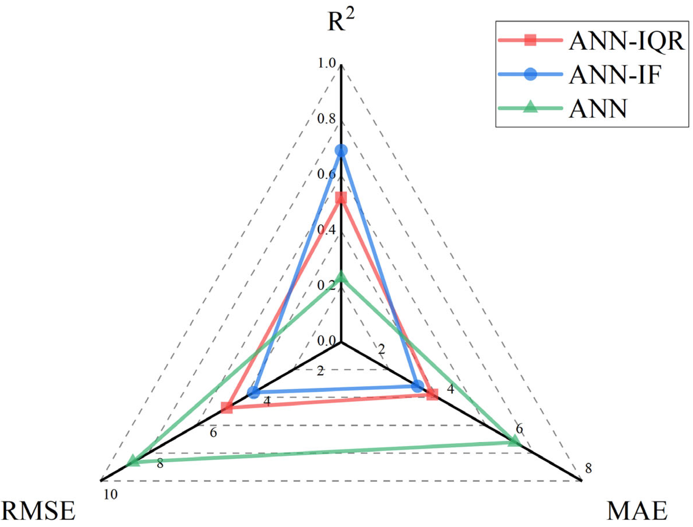
In filtering, using the inter quartile range (IQR = 12.64 (%), Q1 = 49.69 (%) and Q3 = 62.34 (%)), the moisture content smaller than lower bound = 30.72(%) and larger than the upper bound = 81.31(%), were filtered out. After removing these anomaly data, the remaining 404 datasets were used to train the ANN-IQR model. To maintain the similar range of removed data with IQR, anomalous data removal rate for isolation forest was set to 5%. Compared to IQR, anomaly detection of isolation forest is based on the distribution of data instead of the fixed distance. The remain 403 datasets were used to train the ANN-IF model. In addition, the ANN model using all the datasets without removing outliers were also trained to check whether removing outliers can increase the performance indices. The results are shown in Figure 3.
The results show that both methods can significantly improve the accuracy of the model, which means that a small amount of anomalous data may have a great influence on the results. The R2 of IQR and isolation forest increased from 0.23 to 0.52 and 0.69, the MAE decreased from 6.05 to 3.65 and 3.22, and the RMSE decreased from 8.78 to 5.27 and 4.27, respectively. All the performance indices suggested that the isolation forest obtained better accuracy of the model with the datasets. As shown in Figure 2a, the distribution of outliers beyond the upper and lower bounds is uneven. The IQR is based on upper and lower bounds calculated from fixed inter-quartile ranges to detect outliers [41], which creates potential inhomogeneity. In contrast, isolation forest is based on the path length of random division, which can accurately obtain the characteristics of the distribution of anomalous data through calculations. Therefore, the isolation forest was adopted to the later modelling and 23 outliers were removed. In addition, it was also shown that measurement errors and outliers may have a significant influence on prediction results. If possible, it is suggested to use local datasets with consistent measurement accuracy as the basis for modelling.

3.2. Development of ANN Models

3.2.1. Input Parameters

After excluding some models that were less stable during training, 254 ANN models with different parameter combinations selected as inputs are obtained. Due to the stability in the evaluation of different models, the average R2 score in three training process was selected as the final sorting basis. The comparative evaluation of eight ANN models with the best performance is shown in Table 2 In the present study, all performance indices, including R2, MAE and RMSE, were applied to evaluate the relative performance of the models. However, some studies [47] used only the lowest MSE for selection of the best scenario for modelling. The model with input parameters of kitchen, paper, rubber and plastic, bamboo and wood, dust, and metal waste (Model 1) had the R2 of 0.75, MAE of 2.87 and RMSE of 3.84, which represents the most accurate performance among these models.
In all 254 models, the R2 varied from 0.2 to 0.7, the MAE varied from 2.9 to 6.5 and the RMSE varied from 3.8 to 13.6. However, all the evaluation results showed large volatility. It can be seen that different combinations of features have a significant effect on the prediction results. According to previous studies in Section 3.1.2, modelling all compositions as input parameters had poor prediction accuracy (R2 = 0.23, MAE = 6.05, and RMSE = 8.78) comparing with above models, which indicated that the correlations between the input parameters and some input parameters may have a negative influence on the evaluation results. As expected, most of the relevant studies did not use all input parameters to develop models [41]. Therefore, Model 1 was optimized as the final model.

3.2.2. Performance of ANN Model

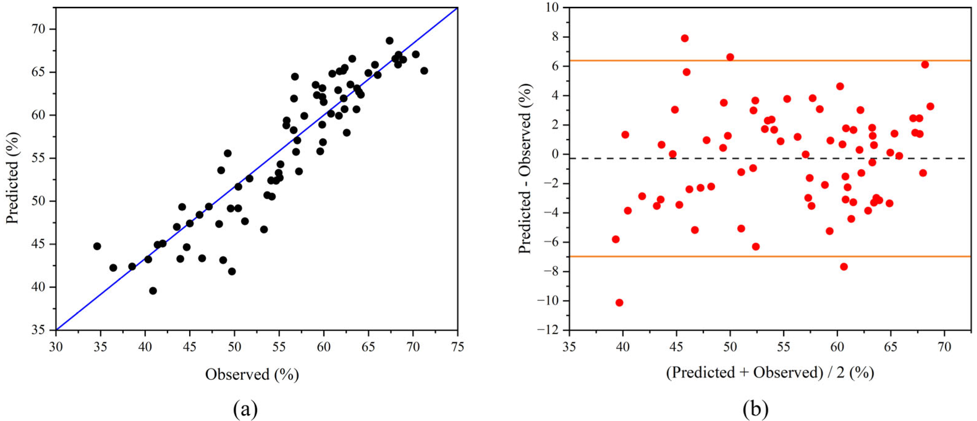
Based on the best input parameters obtained in Section 3.2.1, the number of neurons, activation function, optimization algorithm, learning rate and the max epoch was adjusted by Keras Tuner to determine the optimal ANN model. The final results showed that the neurons number of 8, ReLU activation function, 0.01 as the initial learning rate, and early-stop led to the best prediction results (MAE = 2.67, RMSE = 3.29, R2 = 0.83). The predictions of the model are acceptable for the criteria of evaluation indicators proposed by other researchers [48], which illustrates the mapping relationship between the physical composition of MSW and moisture content.
The predicted-observed plot of moisture content indicated stronger correlation between the predictions of moisture content and its actual observations, which are shown in Figure 4a. As shown in Figure 4b, Bland–Altman plots demonstrated low bias in 95% confidence interval, which means acceptable data consistency. In addition, both figures show that reliable prediction results were obtained at the low and high moisture content, which suggest general applicability of the model.

3.2.3. Uncertainty

The division of training, validation, and test sets introduce uncertainty into the ANN modelling. In addition, uncertainty can be introduced due to the inherent errors of sampling and analyzing [27]. In order to verify the generalization ability and the sensitivity to measurement errors of models, it is necessary to use uncertainty analysis methods.
K-fold cross-validation is an efficient approach to reduce the uncertainty derived from dataset partition. However, there is no definite criterion for the number of subsets to be divided for cross-validation. Abbasi, Rastgoo and Nakisa [46] made an eight-fold cross-validation to verify the uncertainty. The eight-fold cross-validation is shown in Table 3.
The statistical indicators of eight-fold cross-validation show that for the R2, the maximum of eight validations is 0.88, the minimum is 0.53, and the standard deviation is 0.11. With the exceptions of Fold 2 and 3, R2 among different folds was constant ranging from 0.71 to 0.88. However, RMSE is scale dependent and is more sensitive to outliers since errors are squared [49]. Therefore, the coefficient of variation of RMSE is slightly larger than that of R2 (0.17 and 0.15, respectively). The abnormal results of Fold 2 and 3 suggested the presence of outliers in these divided datasets. This result indicates that there is some volatility in dataset partitioning over the eight validations, but data fluctuation is acceptable. Because dataset is ranked by year in cross-validation, and it is not shuffled in advance. The results reflect the temporal variation of moisture content or measurement errors on the time series. Therefore, a more in-depth study of the time series relationship between moisture content and physical composition is recommended.
The robustness of a model is usually defined as the ability to fight against input perturbations and to maintain stable result output [50]. Tests of robustness are often needed in modelling based on small datasets for generalizing their applicability to different scenarios. According the method of Ma, Zhou, Chi, Liu and Yang [27], introducing ±20% noise for each of the four largest components and test their prediction results (the model still uses the best hyperparameters). With the exception of kitchen waste (R2 decreased by 29% and 41%, respectively), changes in the remaining components had essentially no effect on the model results. As the component with the highest weight share in the mixed waste, the error and uncertainty in the measurement of kitchen waste have the greatest effect on the model prediction. Ensuring the accuracy of the measurement of kitchen waste is most important for the generalization performance of model. Therefore, it merits future studies to integrate bottom-p and top-down approaches for reaching high-fidelity MSW parameters datasets.

3.3. Key Components of Functional Areas

Previous experiments in Section 3.1.1 have shown the differences in moisture content and physical composition in different functional areas. It is possible to infer the underlying characteristics and key components in four functional areas through the prediction results.
Parameter exclusion method analyzed the effect of input parameters on the results by developing different models. According to Wu, Niu, Dai and Wu [28], one parameter was excluded every single experiment and the remaining input parameters were used to model. Each time with one predictor omitted. It is assumed that for each parameter, accuracy would be worse when the parameter matters more, and better when it matters less. Consideration of the positive and negative signs of R2, only RMSE and R2 of models with exclusive parameters are given in Figure 5. The evaluation indices of models with all input parameters are marked by the dashed line, and the influence of each component in different functional areas can be analyzed via increasing or decreasing of MAE and RMSE.
The component which had largest weight in the waste, such as kitchen waste, showed the greatest influence on moisture content in residential, cleaning and commercial areas. On the contrary, those components which had lighter weights, such as metals, mix and other wastes, showed poor effects on moisture content in most functional areas. The results indicated that the weight of waste has an important influence on the moisture content in most urban areas.
In residential areas, the model excluding kitchen waste with MAE of 4.23 and RMSE of 7.54 showed the greatest variation (increased 24.4% and 46.8%, respectively), compared with the model of all input parameters. Rubber and plastic waste (increased 10.1% and 19.7%, respectively) also showed positive impacts on moisture content. The result was in line with the habits of most urban citizens, and the same results were obtained in commercial area because of the large amount of waste generation from restaurants and retail businesses. In addition, it can be seen that wood and bamboo, dust and ceramic waste have negative influences on moisture content, which suggests that these disturbing components should be excluded when considering predictions of moisture content in these functional areas.
The results in cleaning area were special, which showed a different pattern of influence than residential and commercial areas. All components had positive impacts on moisture content, which indicated the diversity of influencing factors in cleaning areas. In these components, wood and bamboo waste with MAE of 13.65 and RMSE of 19.09 became the greatest influencing factor (increased 95.3% and 138.1%, respectively). It is easy to explain that tree branches, leaves and dust are the most important sources of street sweeping waste, and due to the complexity of the cleaning scenario, the composition and moisture content of waste shows large variations. However, paper, rubber and plastic, and textile wastes are the three most important components in office areas. Office and transactional matters usually generate a lot of paper waste, which becomes the most important source of waste in office areas.
The influence of MSW composition on moisture content varied significantly in different functional areas. The special relationship between MSW composition and moisture content in urban areas must be considered. With the benefit of the model developed in 3.2, it is easy to encode functional areas as input parameters for modeling.

4. Conclusions

The distribution and generation of MSW is influenced by functional areas, which leading to different relationship between MSW composition and moisture content. In descending order, the moisture content was ranked as commercial/residential > office > cleaning areas. Based on parameter exclusion method, we analyzed the influence on moisture content prediction model of MSW composition in these areas. Kitchen waste was the most important parameter of MSW composition in most functional areas. In residential and commercial area, kitchen, rubber, and plastic wastes showed the greatest influence on moisture content. In cleaning area, wood and bamboo wastes were the most important indices, and paper waste in office area.
With functional areas encoded as input parameters, a fast and widely applicable ANN model to predict moisture content in MSW was developed. The final ANN model with the R2 of 0.83, MAE of 2.67 and RMSE of 3.29 obtained rewarding evaluation results, which showed that the models based on ANN exhibited acceptable and compatible levels of performance. As an effective anomaly data detection method, isolation forest was more suitable to reduce the influence of extreme data, especially in volatile datasets compared with the IQR filter.
With the benefit of the one-hot code of functional areas, we can develop just one model to consider the impact of all functional areas as best practice. In addition, because of the large differences in key components in different functional areas, the determination of key components in different functional areas will be helpful for reducing the workload of moisture content estimation.

Author Contributions

Conceptualization, T.H.; methodology, T.H.; software, T.H.; validation, T.H.; formal analysis, T.H.; investigation, T.H. and G.C.; resources, D.N.; data curation, D.N.; writing—original draft preparation, T.H.; writing—review and editing, D.N., F.W. and Y.C.; visualization, T.H. and G.C.; supervision, D.N., F.W. and Y.C.; project administration, D.N.; funding acquisition, D.N. All authors have read and agreed to the published version of the manuscript.

Funding

This research was financially supported by the National Key Technologies R&D Program of China (Grant No.2019YFC1904002).

Data Availability Statement

Not applicable.

Conflicts of Interest

The authors declare no conflict of interest.

Abbreviations

MSWmunicipal solid waste
ANNartificial neural network
IQRinter quartile range
IFisolation forest
MAEmean absolute error

References

  1. Xue, B.; Geng, Y.; Ren, W.X.; Zhang, Z.L.; Zhang, W.W.; Lu, C.Y.; Chen, X.P. An overview of municipal solid waste management in Inner Mongolia Autonomous Region, China. J. Mater. Cycles Waste Manag. 2011, 13, 283–292. [Google Scholar] [CrossRef]
  2. Marousek, J. Economically oriented process optimization in waste management. Environ. Sci. Pollut. Res. Int. 2014, 21, 7400–7402. [Google Scholar] [CrossRef] [PubMed]
  3. Sha’Ato, R.; Aboho, S.Y.; Oketunde, F.O.; Eneji, I.S.; Unazi, G.; Agwa, S. Survey of solid waste generation and composition in a rapidly growing urban area in Central Nigeria. Waste Manag. 2007, 27, 352–358. [Google Scholar] [CrossRef] [PubMed]
  4. Ibikunle, R.A.; Lukman, A.F.; Titiladunayo, I.F.; Haadi, A.-R.; Pham, D.T. Modeling energy content of municipal solid waste based on proximate analysis: R-k class estimator approach. Cogent Eng. 2022, 9, 2046243. [Google Scholar] [CrossRef]
  5. Shi, H.H.; Mahinpey, N.; Aqsha, A.; Silbermann, R. Characterization, thermochemical conversion studies, and heating value modeling of municipal solid waste. Waste Manag. 2016, 48, 34–47. [Google Scholar] [CrossRef] [PubMed]
  6. Tumuluru, J.S.; Yancey, N.A.; Kane, J.J. Pilot-scale grinding and briquetting studies on variable moisture content municipal solid waste bales—Impact on physical properties, chemical composition, and calorific value. Waste Manag. 2021, 125, 316–327. [Google Scholar] [CrossRef]
  7. Ding, C.X.; Yan, A.J. Fault Detection in the MSW Incineration Process Using Stochastic Configuration Networks and Case-Based Reasoning. Sensors 2021, 21, 7356. [Google Scholar] [CrossRef]
  8. Wang, D.; Tang, Y.T.; He, J.; Yang, F.; Robinson, D. Generalized models to predict the lower heating value (LHV) of municipal solid waste (MSW). Energy 2021, 216, 119279. [Google Scholar] [CrossRef]
  9. Shu, H.-Y.; Lu, H.-C.; Fan, H.-J.; Chang, M.-C.; Chen, J.-C. Prediction for energy content of Taiwan municipal solid waste using multilayer perceptron neural networks. J. Air Waste Manag. Assoc. 2006, 56, 852–858. [Google Scholar] [CrossRef]
  10. Mushtaq, J.; Dar, A.Q.; Ahsan, N. Physio-chemical characterization of municipal solid waste and its management in high-altitude urban areas of North-Western Himalayas. Waste Dispos. Sustain. Energy 2020, 2, 151–160. [Google Scholar] [CrossRef]
  11. Mushtaq, J.; Dar, A.Q.; Ahsan, N. Spatial–temporal variations and forecasting analysis of municipal solid waste in the mountainous city of north-western Himalayas. SN Appl. Sci. 2020, 2, 1161. [Google Scholar] [CrossRef]
  12. Chang, Y.F.; Lin, C.J.; Chyan, J.M.; Chen, I.M.; Chang, J.E. Multiple regression models for the lower heating value of municipal solid waste in Taiwan. J. Environ. Manag. 2007, 85, 891–899. [Google Scholar] [CrossRef]
  13. Drudi, K.C.R.; Drudi, R.; Martins, G.; Antonio, G.C.; Leite, J.T.C. Statistical model for heating value of municipal solid waste in Brazil based on gravimetric composition. Waste Manag. 2019, 87, 782–790. [Google Scholar] [CrossRef] [PubMed]
  14. Ni, L.J.; Zhang, G.L.; Ruan, X.L.; Zhao, W.J.; Zhou, L.X. The flux and pollution character of dust-fall in different functional zones of Nanjing. China Environ. Sci. 2007, 27, 2–6. [Google Scholar]
  15. Pan, W.; He, Q.; Li, G.; Ai, H.; Liu, L. Study on characteristics of sewer sediments in a mountainous city. China Environ. Sci. 2014, 34, 1485–1490. [Google Scholar]
  16. Sekhavatjou, M.S.; Alhashemi, A.H.; Rostami, A. Comparison of Trace Element Concentrations in Ambient Air of Industrial and Residential Areas in Tehran City. Biol. Trace Elem. Res. 2011, 143, 1413–1423. [Google Scholar] [CrossRef]
  17. Chen, H.; Gong, C.; Li, W. Characteristic and Evaluation of Soil Pollution by Heavy Metalin Different Functional Zones of Guangzhou. J. Environ. Health 2010, 27, 700–703. [Google Scholar]
  18. Liu, Y.-N.; Zhu, S.-F.; Wei, X.-F.; Miao, J.; Zhou, M.; Guan, F.-J. Assessment and Pollution Characteristics of Heavy Metals in Soil of Different Functional Areas in Luoyang. Huan Jing Ke Xue Huanjing Kexue 2016, 37, 2322–2328. [Google Scholar] [CrossRef]
  19. Ni, J.; Chen, W.; Yang, H.; Wei, R.; Yang, Y. Concentrations and sources of soil PAHs in various functional zones of Fuzhou City. China Environ. Sci. 2012, 32, 921–926. [Google Scholar]
  20. Shirokikh, I.G.; Solov’eva, E.S.; Ashikhmina, T.Y. Actinomycete complexes in soils of industrial and residential zones in the city of Kirov. Eurasian Soil Sci. 2014, 47, 89–95. [Google Scholar] [CrossRef]
  21. Ullah, S.; Bibi, S.D.; Ali, S.; Noman, M.; Rukh, G.; Nafees, M.A.; Bibi, H.; Ali, S.; Qiao, X.C.; Khan, S.; et al. Analysis of municipal solid waste management in afghanistan, current and future prospects: A case study of kabul city. Appl. Ecol. Environ. Res. 2022, 20, 2485–2507. [Google Scholar] [CrossRef]
  22. Kumar, U.A. Comparison of neural networks and regression analysis: A new insight. Expert Syst. Appl. 2005, 29, 424–430. [Google Scholar] [CrossRef]
  23. Soni, U.; Roy, A.; Verma, A.; Jain, V. Forecasting municipal solid waste generation using artificial intelligence models—A case study in India. SN Appl. Sci. 2019, 1, 162. [Google Scholar] [CrossRef] [Green Version]
  24. Kumar, A.; Samadder, S.R.; Kumar, N.; Singh, C. Estimation of the generation rate of different types of plastic wastes and possible revenue recovery from informal recycling. Waste Manag. 2018, 79, 781–790. [Google Scholar] [CrossRef] [PubMed]
  25. Golbaz, S.; Nabizadeh, R.; Sajadi, H.S. Comparative study of predicting hospital solid waste generation using multiple linear regression and artificial intelligence. J. Environ. Health Sci. Eng. 2019, 17, 41–51. [Google Scholar] [CrossRef] [PubMed]
  26. Ye, G.; Luo, H.; Ren, Z.; Ahmad, M.S.; Liu, C.-G.; Tawab, A.; Al-Ghafari, A.B.; Omar, U.; Gull, M.; Mehmood, M.A. Evaluating the bioenergy potential of Chinese Liquor-industry waste through pyrolysis, thermogravimetric, kinetics and evolved gas analyses. Energy Convers. Manag. 2018, 163, 13–21. [Google Scholar] [CrossRef]
  27. Ma, S.; Zhou, C.; Chi, C.; Liu, Y.; Yang, G. Estimating Physical Composition of Municipal Solid Waste in China by Applying Artificial Neural Network Method. Environ. Sci. Technol. 2020, 54, 9609–9617. [Google Scholar] [CrossRef]
  28. Wu, F.; Niu, D.; Dai, S.; Wu, B. New insights into regional differences of the predictions of municipal solid waste generation rates using artificial neural networks. Waste Manag. 2020, 107, 182–190. [Google Scholar] [CrossRef]
  29. Adamovic, V.M.; Antanasijevic, D.Z.; Cosovic, A.R.; Ristic, M.D.; Pocajt, V.V. An artificial neural network approach for the estimation of the primary production of energy from municipal solid waste and its application to the Balkan countries. Waste Manag. 2018, 78, 955–968. [Google Scholar] [CrossRef]
  30. Dong, C.Q.; Jin, B.S.; Li, D.J. Predicting the heating value of MSW with a feed forward neural network. Waste Manag. 2003, 23, 103–106. [Google Scholar] [CrossRef]
  31. Lin, C.-J.; Chyan, J.-M.; Chen, I.M.; Wang, Y.-T. Swift model for a lower heating value prediction based on wet-based physical components of municipal solid waste. Waste Manag. 2013, 33, 268–276. [Google Scholar] [CrossRef] [PubMed]
  32. Zhao, Y.C.; Stucki, S.; Ludwig, C.; Wochele, J. Impact of moisture on volatility of heavy metals in municipal solid waste incinerated in a laboratory scale simulated incinerator. Waste Manag. 2004, 24, 581–587. [Google Scholar] [CrossRef]
  33. Suksankraisorn, K.; Patumsawad, S.; Fungtammasan, B. Co-firing of Thai lignite and municipal solid waste (MSW) in a fluidised bed: Effect of MSW moisture content. Appl. Therm. Eng. 2010, 30, 2693–2697. [Google Scholar] [CrossRef]
  34. Meng, A.H.; Li, Q.H.; Jia, J.Y.; Zhang, Y.G. Effect of Moisture on Partitioning of Heavy Metals in Incineration of Municipal Solid Waste. Chin. J. Chem. Eng. 2012, 20, 1008–1015. [Google Scholar] [CrossRef]
  35. Sebastian, R.M.; Kumar, D.; Alappat, B.J. Easy Estimation of Mixed Municipal Solid Waste Characteristics from Component Analysis. J. Environ. Eng. 2019, 145. [Google Scholar] [CrossRef]
  36. Wang, G.; Zhang, H.; Wang, D.; Zhang, L.; Sun, W. Physical composition and characteristics analysis of the municipai solid waste (MSW) in Beijing. Environ. Eng. 2018, 36, 132–136. [Google Scholar]
  37. Bolukbas, A.; Akinci, G. Solid waste composition and the properties of biodegradable fractions in Izmir City, Turkey: An investigation on the influencing factors. J. Environ. Health Sci. Eng. 2018, 16, 299–311. [Google Scholar] [CrossRef] [PubMed]
  38. Pawara, P.; Okafor, E.; Groefsema, M.; He, S.; Schomaker, L.R.B.; Wiering, M.A. One-vs-One classification for deep neural networks. Pattern Recognit. 2020, 108, 107528. [Google Scholar] [CrossRef]
  39. Klimo, M.; Lukac, P.; Tarabek, P. Deep Neural Networks Classification via Binary Error-Detecting Output Codes. Appl. Sci. 2021, 11, 3563. [Google Scholar] [CrossRef]
  40. Liu, F.T.; Ting, K.M.; Zhou, Z.-H. Isolation-Based Anomaly Detection. ACM Trans. Knowl. Discov. Data 2012, 6, 1–39. [Google Scholar] [CrossRef]
  41. Fallah, B.; Ng, K.T.W.; Vu, H.L.; Torabi, F. Application of a multi-stage neural network approach for time-series landfill gas modeling with missing data imputation. Waste Manag. 2020, 116, 66–78. [Google Scholar] [CrossRef]
  42. Xu, D.; Wang, Y.; Meng, Y.; Zhang, Z. An Improved Data Anomaly Detection Method Based on Isolation Forest. In Proceedings of the 2017 10th International Symposium on Computational Intelligence and Design (ISCID), Hangzhou, China, 9–10 December 2017; pp. 287–291. [Google Scholar]
  43. Prechelt, L. Automatic early stopping using cross validation: Quantifying the criteria. Neural Netw. 1998, 11, 761–767. [Google Scholar] [CrossRef] [Green Version]
  44. Behera, S.K.; Meher, S.K.; Park, H.-S. Artificial neural network model for predicting methane percentage in biogas recovered from a landfill upon injection of liquid organic waste. Clean Technol. Environ. Policy 2015, 17, 443–453. [Google Scholar] [CrossRef]
  45. Kannangara, M.; Dua, R.; Ahmadi, L.; Bensebaa, F. Modeling and prediction of regional municipal solid waste generation and diversion in Canada using machine learning approaches. Waste Manag. 2018, 74, 3–15. [Google Scholar] [CrossRef] [PubMed]
  46. Abbasi, M.; Rastgoo, M.N.; Nakisa, B. Monthly and seasonal modeling of municipal waste generation using radial basis function neural network. Environ. Prog. Sustain. Energy 2019, 38, e13033. [Google Scholar] [CrossRef]
  47. Moghaddamnia, A.; Remesan, R.; Kashani, M.H.; Mohammadi, M.; Han, D.; Piri, J. Comparison of LLR, MLP, Elman, NNARX and ANFIS Models-with a case study in solar radiation estimation. J. Atmos. Sol.-Terr. Phys. 2009, 71, 975–982. [Google Scholar] [CrossRef]
  48. Coulibaly, P.; Baldwin, C.K. Nonstationary hydrological time series forecasting using nonlinear dynamic methods. J. Hydrol. 2005, 307, 164–174. [Google Scholar] [CrossRef]
  49. Vu, H.L.; Ng, K.T.W.; Richer, A.; An, C.J. Analysis of input set characteristics and variances on k-fold cross validation for a Recurrent Neural Network model on waste disposal rate estimation. J. Environ. Manag. 2022, 311, 114869. [Google Scholar] [CrossRef]
  50. Thompson, M.P.; Kambhampati, C. Increasing innate robustness in artificial neural networks using redundancy. Electron. Lett. 1995, 31, 1931–1932. [Google Scholar] [CrossRef]
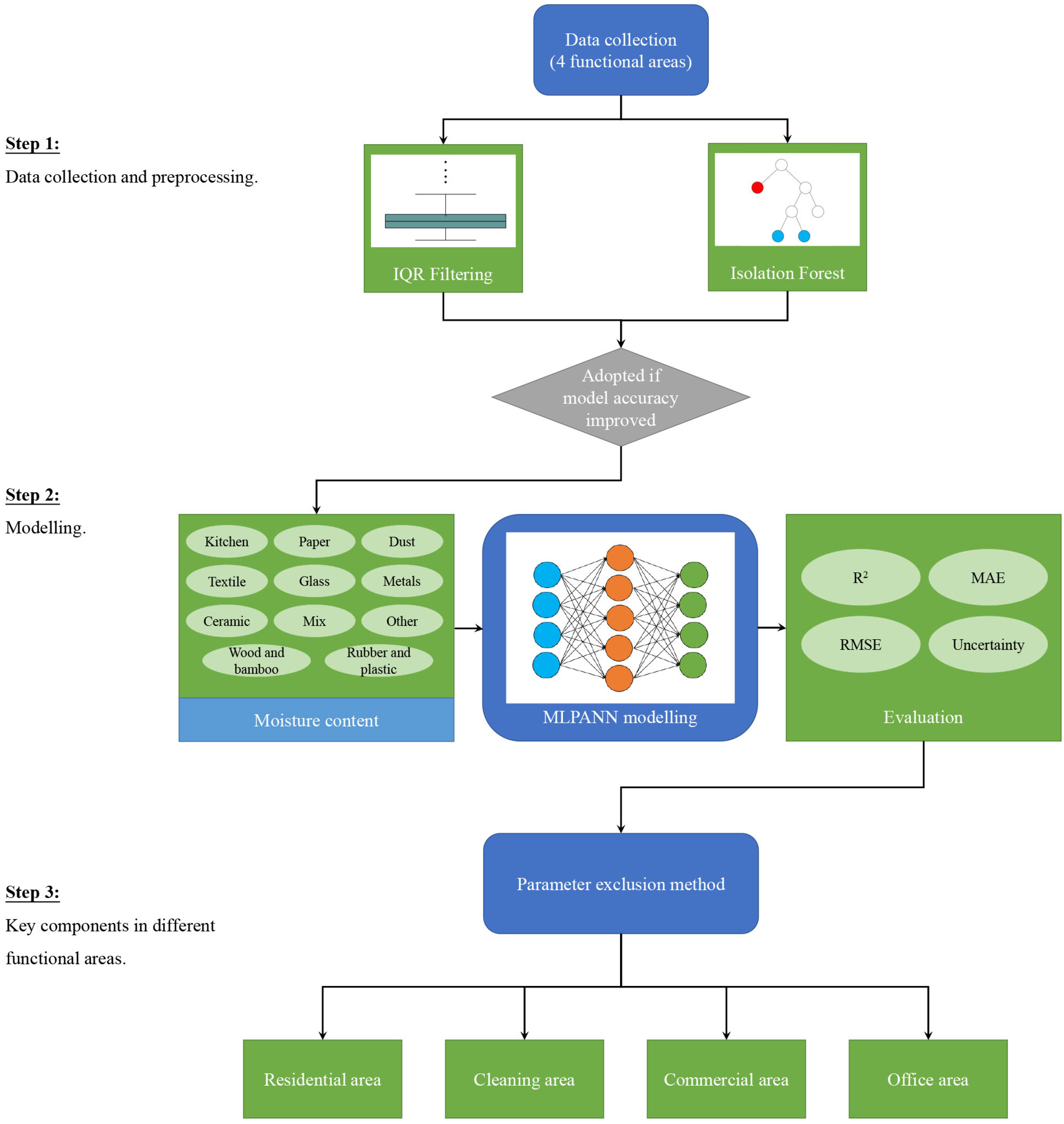
Figure 1. Flowchart for moisture content modelling and key components exploring in four function areas.
Sustainability 14 15544 g001
Figure 2. The box plot (a) of MSW moisture content and circle plot (b,c) of MSW composition.
Sustainability 14 15544 g002
Figure 3. Model performance of MSW moisture content with IQR and Isolation Forest.
Sustainability 14 15544 g003
Figure 4. The predicted-observed plot (a) of moisture content and Bland-Altman plots (b) in 95% confidence interval of moisture content.
Sustainability 14 15544 g004
Figure 5. MAE and RMSE of parameter exclusion analysis in different functional areas.
Sustainability 14 15544 g005
Table 1. Dataset statistics of input data (%).
MaxMean25% a50% b75% cMinStdStd/Mean
Moisture content95.6854.6249.7057.7962.340.0013.050.24
Kitchen waste84.8457.5849.7660.4368.960.0014.510.25
Paper waste37.6111.758.1011.0014.470.995.240.45
Rubber and plastic waste44.8217.8613.8617.2021.004.935.450.31
Textile waste60.762.220.801.642.580.004.061.83
Wood and bamboo waste93.676.230.450.902.620.0014.232.29
Dust waste6.610.040.000.000.000.000.379.07
Ceramic waste5.680.300.000.090.370.000.612.01
Glass waste12.522.361.042.153.280.001.900.80
Metals waste5.940.690.170.470.930.000.741.08
Other waste8.820.090.000.000.020.000.566.11
Mix waste24.590.450.000.000.000.002.064.62
a,b,c The 25%, 50% and 75% mean 25, 50 and 75 percent of datasets are less than the corresponding values.
Table 2. The best 8 models of MSW moisture content with batched modelling.
Evaluation IndicesModel1Model2Model3Model4Model5Model6Model7Model8
R20.740.730.7250.720.7150.710.7050.7
MAE2.953.083.0253.0353.123.0953.13.2
RMSE3.8953.984.024.054.064.1154.1454.15
Table 3. R2, MAE and RMSE for model fitting in each fold of cross validation.
Fold1Fold2Fold3Fold4Fold5Fold6Fold7Fold8
R20.8830.7490.5290.5360.7190.7130.7640.744
MAE2.7253.3704.2833.8083.5442.7653.1353.157
RMSE3.3604.1245.7554.8514.4973.4504.0574.024
Publisher’s Note: MDPI stays neutral with regard to jurisdictional claims in published maps and institutional affiliations.