Flood Susceptibility Mapping Using Watershed Geomorphic Data in the Onkaparinga Basin, South Australia

Abstract

In the near future, natural disasters and associated risks are expected to increase, mainly because of the impact of climate change. Australia is considered one of the most vulnerable areas for natural disasters, including flooding. Therefore, an evaluation of the morphometric characteristics of the Onkaparinga basin in South Australia was undertaken using the integration of remote sensing and geospatial techniques to identify its impact on flash floods. The Shuttle Radar Topography Mission (SRTM) and Landsat images with other available geologic, topographic, and secondary data were analysed in geographic information system (GIS) to outline the drainage basins, estimate the morphometric parameters, and rank the parameters to demarcate the flash flood susceptibility zones of the basin. The main goal was to develop a flash flood susceptibility map showing the different hazard zones within the study areas. The results showed that 10.87%, 24.27%, and 64.85% are classified as low, moderate, and highly susceptible for flooding, respectively. These findings were then verified against secondary data relating to the historic flood events of the area. About 30.77% of the historical floods are found located within the high to extremely susceptible zones. Moreover, a significant correlation has been found between the high precipitation concentration index (PCI) and the irregular rainfall and high potential for flooding. Finally, the social and economic vulnerability was applied to determine the impact of the flood hazards. The result indicates a widespread threat to the economy, environment, and community in the study area. This study can be utilized to support and assist decision makers with planning and the devotion of alleviation measures to reducing and avoiding catastrophic flooding events, especially in highly susceptible areas in the world, such as South Australian basins.

1. Introduction

In recent decades, extreme weather events became one of the most hazardous environmental phenomena [1]. It has caused the death of thousands of people and, due to damage, the loss of AUD hundreds of millions on average per year worldwide [1,2,3]. The environmental and socioeconomic consequences of these events is very significant in Australia [4]. According to recent research, the direct costs from extreme weather events are estimated to increase by 5.13% each year, which causes economic loss to increase to AUD 35.24 billion (in 2022 AUD) by 2050 [5].

Flood is considered a devastating natural disaster. During the last few decades, it has been evident that global warming and climate change have caused an increase in the frequency and intensity of extreme rainfall [6]. As a result, the magnitude and risk of flooding has increased and developed into a critical issue for life, properties and infrastructure [7]. Therefore, the analysis of flood susceptibility is essential for efficient prevention and mitigation of future hazard events, especially in recent years, as extreme precipitation and flood intensity occurs as a result of global warming and climate change. Flood risk management is challenging due to the interactions between different factors [8]. There are numerous environmental and man-made factors that influence flood occurrences in a region [9]. Generally, flood-generating factors include meteorological conditions, such as intense rainfall, and geomorphometric features, including gradient, area, and the shape of the watershed, as well as other parameters, such as land use, land cover, and soil permeability [10]. Floods are primarily caused by extreme rainfall events on site or upstream and are then intensified by other factors, such as the duration and patterns of the rainfall [11]. It is also influenced by the hydraulic characteristics of the catchment and their extreme response to rainfall, resulting from their steep slopes and high drainage density [12]. Moreover, low permeable soils could accelerate the surface runoff and suddenly decrease the lag time required for the genesis of floods [13] Similarly, changes in land use and urbanization may further increase the flood susceptibility in any catchment [14]. As a result, a devastating flood can be generated from the complicated interaction of hydrologic and climatic conditions with the landscapes and morphological features of the watershed [15].

Many studies were carried out to understand this interaction and evaluate the severity of risk at regions susceptible to floods [16,17,18]. In the literature, there is no straightforward set of standards of geomorphometric specifications that can be used for identifying the flood susceptibility zones [19]. Nonetheless, it is obvious that combinations of these parameters can be effectively used to define flood hazard zones [19,20,21,22,23]. Thus, a geomorphometric analysis, which plays a vital role in predicting floods, is commonly used as a quantitative method in evaluating and assessing sub-basin characteristics [24]. Basin geomorphometric parameters could provide us with significant information towards the characterization of devastating hydro-meteorological hazards, such as floods [25].

At present, these parameters can be obtained from remotely sensed data (RS) analysis in a geographic information system (GIS) environment [25]. Sensed data (RS) and GIS techniques provide us with time and a cost-effective solution to understand, evaluate, manipulate, and delineate potential flood hazard areas [26,27]. These techniques are widely applied to evaluate and assess flood-related damages caused by extreme rain events in a catchment area [28,29,30]. It is also considered as a reliable method for accurately predicting flood [31]. It has often been integrated with the analytical hierarchy process (AHP) [32,33,34], weights of evidence (WOE) [35,36], multi-criteria decision approach (MCDA) [26,37,38], artificial neural networks (ANN) [39,40], adaptive neuro–fuzzy interface system [41,42], logistic regression (LR) [43], and fraction ratio (FR) model [9]. These methods and techniques are widely known acceptable models for flooding hazard analysis. This study is a trial to validate the regional study for mapping the flood susceptibility areas using the geomorphic analysis as a robust method in the South Australian basins. The value of the previous work was limited by the large basin characteristics, which, in turn, impacted the results and produced superior expectation to differ at a finer or smaller scale. For example, at a smaller scale, water flow, velocity, and quantity are supposed to have a direct link with some geomorphic aspects, such as relief and form indices. Therefore, the aim of the present study is to investigate the usefulness of remote sensing (RS), GIS, and the geomorphic analysis for flood susceptibility mapping in the Onkaparinga area, which was considered here as a relatively small-scale basin, validating the final flood susceptibility map using the historical and rainfall indices and evaluating the flood hazard using the available demographic data.

2. Materials and Methods

2.1. Floods in Australia

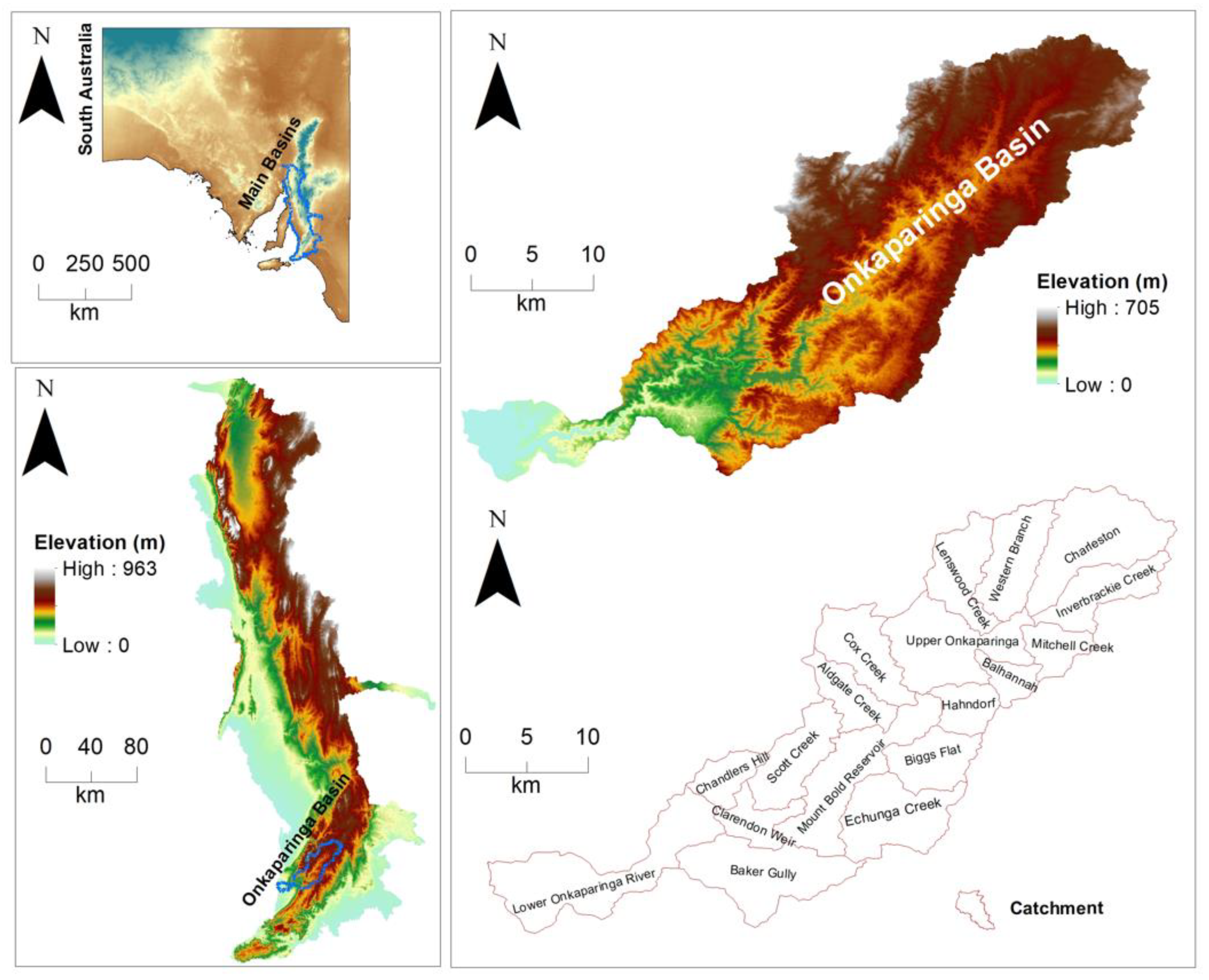
In Australia, floods frequently occur; thus, records of floods are dated back to 1836. In most cases, they are attributed to climatic triggers, such as orographic uplift causing a heavy, prolonged rainfall event; convective vertical motion; frontal and banded vertical motion; low level convergence/upper divergence; storm surges; seasonal variation; and influence of El Nino southern oscillation [44]. Moreover, geological landforms and soil factors could result in variations in floodplain extent and nature of the flood hazard [23]. These events caused human losses and economic damage across the country. For example, 2292 flood fatalities were recorded for the period from 1790 to 2001 while AUD 10.4 billion was estimated as the total cost of flooding in the period from 1967 to 1999 [45]. In south Australia, between 1870 and 1956, River Murray floods were classified as the most devastating flood events. Another recent example is the Gawler River flood in 2006, which caused over AUD 40 million in losses of crops, property, and infrastructure. Due to such socioeconomic and demographic consequences, more research is needed to understand and manage the flood risks, which is a significant problem for the urbanized areas of Australia. It is very important to understand flood hydrology and geomorphic changes and develop an accurate flood susceptibility map as a tool to understand and manage the flood risks.

2.2. Study Area

The Onkaparinga River Basin is located 30 km east of Adelaide (Figure 1). The basin extends between 35°00′ to 35°10′ S latitudes and 138°25′ to 139°00′ E longitudes and exhibits a dendritic stream pattern (Figure 1). The river originates from Mount Torrens in the Mount lofty Ranges and flows south westerly towards the Gulf of Saint Vincent at Port Noarlunga. The main sub-basins of the Onkaparinga River are Aldgate, Lenswood, Echunga creeks, Inverbrackie, and Cox. The major towns in the basin are Hahndorf, Lobethal, Bridgewater, Balhannah, and Aldgate. The study area is characterised by a variable topography with low relief in the downstream areas and a variety of erosional landforms, such as dissected hills and ridges in upstream. It ranges from 10 to 700 m and controls the runoff movement during monsoon season.

Today, climate of the basin is arid–semi arid with a cool wet winters and warm dry summers. Rainfall shows a seasonal bias towards winter, with most rain falling between May and September. Rainfall, however, is variable from the 1170 mm in upstream areas to 400 mm near the coast [46]. As part of south Australia, two major drivers are causing the rainfall variability (1) La Niña and (2) El Niño [47]. During the wet summer monsoon, La Niña results from cooling of the tropical eastern and central Pacific Ocean, bringing heavy rain to many parts of Australia. Conversely, an El Niño occurs when the equatorial eastern and central Pacific waters warm, easterly winds in the tropics weaken, and it results in more arid conditions in the region [48,49].

With a total population of 174.575, Onkaparinga (175,711) has the largest population within Greater Adelaide (121,065) (https://population.gov.au/, accessed on 15 November 2022). According to the most recent Census of Population and Housing, which was conducted in 2021, the area grew at faster rate and recorded the highest largest population growth, accounting for a total of 3963 persons. This represents more than double the total population increase in Greater Adelaide (https://www.abs.gov.au/, accessed on 15 November 2022).

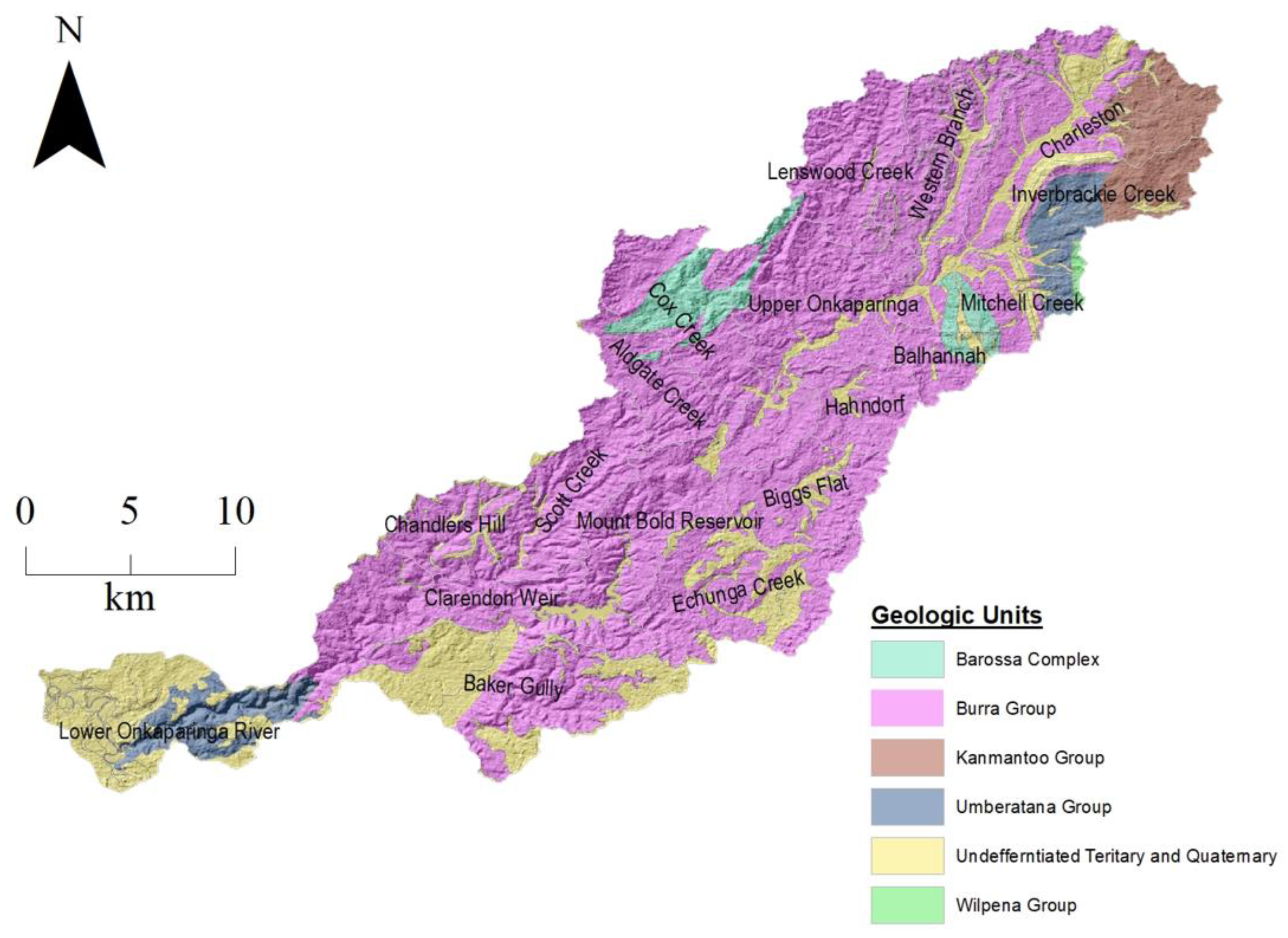
2.3. Geological Setting

The Onkaparinga River Basin is located in the southern Mount Lofty area of South Australia. Geologically, the ranges are part of the Adelaide Geosyncline, which contains varied lithological features, ranging in age from Neoproterozoic to Cambrian [50]. The Onkaparinga Basin is mainly underlain by the Barossa Complex, Adelaidean sediments, Kanmantoo Group, and Quaternary alluvium [51]. The Barossa Complex is the oldest stratigraphic unit and constitutes the basal part of the rock sequence (~500 million years). It comprises consolidated basement rocks overlying the Adelaidean sediments [52]. The basement rocks are outcropped as Aldgate and Oakbank inliers in the centre of large folds, which occurred in the western areas of the study area (Figure 2).

With a thickness of ~24,000 m and of the Precambrian age, the Adelaidean sediments are dominated by the Burra Group, which consists mainly of shale, siltstone, slate, dolomite, sandstone, and quartzite at the basal part of the sedimentary sequence (Figure 2). It is unconformably overlying the Umberatana Group, which subdivided into the older glacial beds (mainly tillite), younger interglacial siltstone and carbonate, and upper glacial beds [52]. The Wilpena Group contains mainly clastic and the Ediacara metazoan assemblage capped by dolomite [52]. The rocks are strongly folded and relatively unmetamorphosed and, therefore, keep a depositional, sedimentological and climatic record [50]. Kanmantoo Group occurred as a large trough of greywacke, schist, and gneiss of Cambrian age with a thickness of ~21,000 m. These metamorphic rocks are outcropped along the eastern parts of the study area. The Quaternary alluvium sediments are found at the lowest points in the catchment, along the Onkaparinga River and other drainage lines. It consists of dark grey clay and silt with inter-bedded sand, gravel, and thin sandstone dominating the upper part [53].

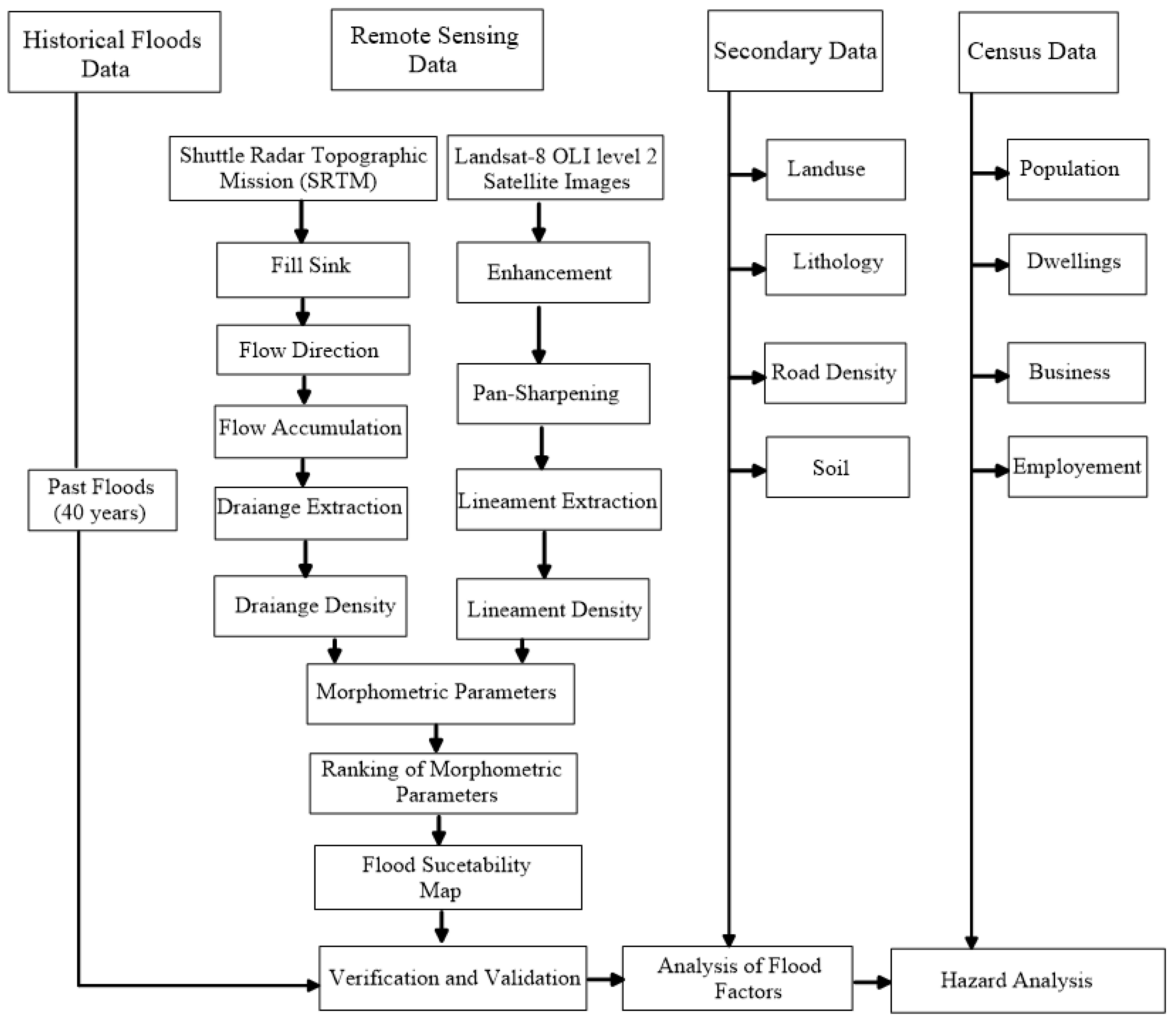
2.4. Data Sources and Processing

In this study, data, from different websites and organizations, are analysed to identify the flash flood susceptibility zones in the Onkaparinga River Basin, South Australia (Figure 3). In the following section, a discussion about the data sources, formats, processing, and analysis are presented. The SRTM (Shuttle Radar Topographic Mission of 30 m resolution) digital elevation model, downloaded from Geoscience Australia, was used to derive geomorphometric parameters for identifying the flood susceptibility zones [54]. The SRTM was processed in a GIS platform by identifying filling sinks, flow direction, flow accumulation grids, and defining watersheds to generate drainage network. Subsequently, a stream order was identified by applying a stream ordering method [55]. The drainage network for the study area was further verified using toposheets in ArcGIS platform. Moreover, the slope map was prepared from SRTM DEM data Spatial Analyst module in ArcGIS.

Landsat-8 OLI level 2 satellite data, acquired from the Global Landcover Facility (GLCF) on 3 December 2022, were used to determine the best discrimination of the lineaments using an optimum False Color Composite (7, 4, and 2 in red, green, and blue) image and principal component analysis (PCA). The automatic extraction of lineaments involved mosaicking and enhancement was performed in ENVI TM 5.1, as well as edge detection, thresholding, and curve extraction using the LINE module in PCI Geomatica and exporting lineaments to GIS environment. As line features could be man-made constructions, such as roads or fences, the extracted lineaments were verified using the road network published by the Department of Planning, Transport and Infrastructure, South Australia. Finally, verified lineament layer was used to create density raster map using Line Density tool in Arc Map 10.7.

In this study, a large number of rainfall stations monitored by the Bureau of Meteorology (BoM) are located within and adjacent to the Onkaparinga catchment (44 stations are within the catchment and another 49 adjacent to the catchment). In this study, annual rainfall data from 17 rain stations selected for the period 1991 to 2021 were used to verify and validate the results (Figure 4). These rainfall stations were previously tested for temporal homogeneity by [46] using random checks by Sinclair Knight Merz. They found that the temporal homogeneity of rainfall data at these stations was satisfactory.

Land use classes were obtained and verified using the Australian Land Use and Management Classification Version 8, which was derived from aerial imagery and on-ground field surveys, and available from the South Australian Government Data Web Directory. In addition, lithology, soil, well data, and demographic data were obtained from the South Australian government website (https://data.environment.sa.gov.au/, accessed on 15 November 2022) and clipped in ArcGIS software to prepare thematic layers of the study area.

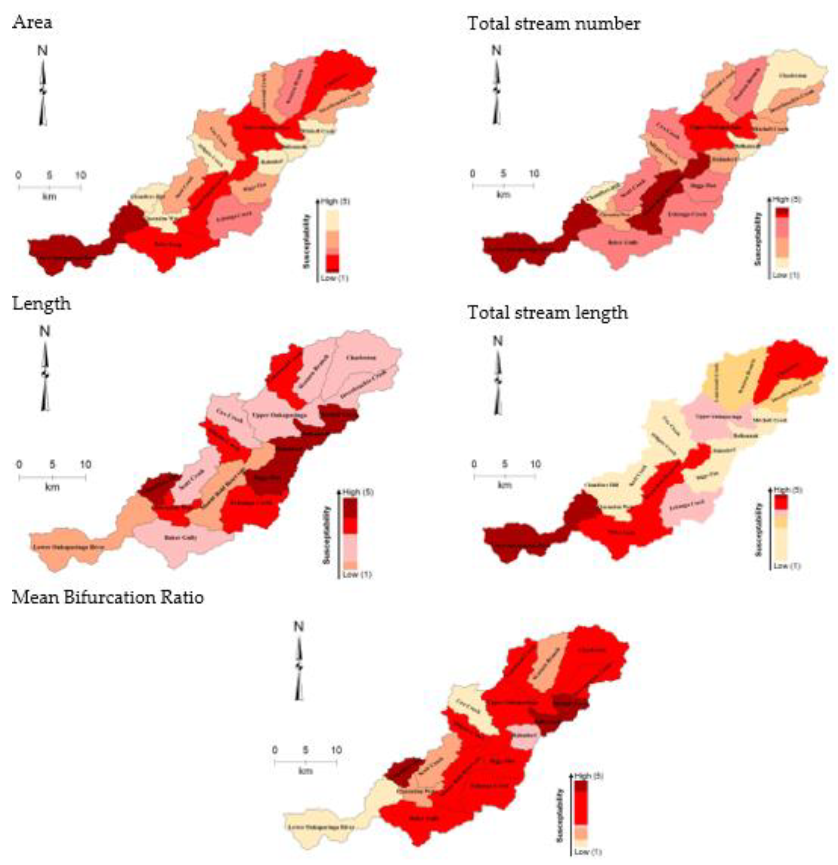
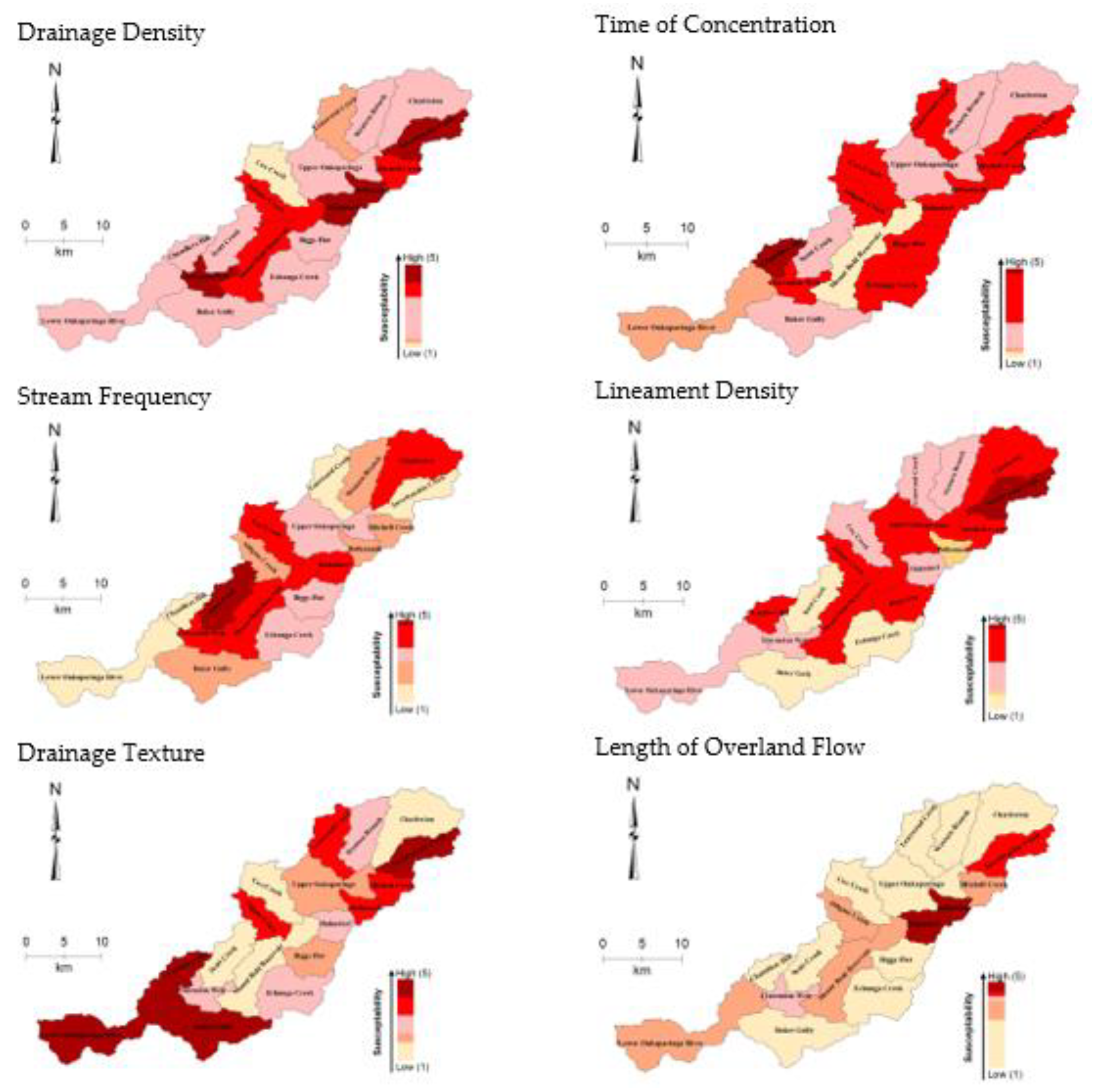
2.5. Ranking Morphometric Parameters for Flash Flood Susceptibility

In order to identify the flash flood susceptibility zones, 19 morphometric parameters, including drainage, linear, shape, texture, and relief characteristics of the Onkaparinga River Basin and its sub-basins, were extracted and calculated using established geomorphological formulas (Table 1). According to the level of flash flood susceptibility, a rank (y) was assigned for each watershed according to the level of flood susceptibility. In this method, 1 and 5 denote very low and very high, respectively, susceptibility in relation to the value of each morphometric parameter (x). A linear interpolation technique proposed by [56] was applied to obtain the susceptibility ranks. If the value of a parameter is positively correlated with the occurrence of flash flood event, then Equation (1) is used. Otherwise, Equation (2) is applied.

Y ∝ x, y′_n = (y₂ − y₁)(x′_n − x_min)/(x_max − x_min) + y₁

(1)

y ∝ 1/x, y′_n = (y₂ − y₁)(x′_n − x_max)/(x_min − x_max) + y₁

(2)

where y′_n is the susceptibility rank of a parameter for the nth watershed (n = 1, 2, 3,..., 33), the maximum rank y₂ = 5, minimum rank y₁ = 1, x′_n is the value of a parameter for the nth watershed, X_max is the maximum value of a parameter among all watersheds, and X_min is the minimum value of a parameter among all watersheds.

2.6. Flood Susceptibility Analysis

Twenty flash flood susceptibility maps for the individual morphometric parameters were used to estimate the total rank of each watershed in the Onkaparinga River Basin. Then, the aggregated map was categorized (using Equations (1) and (2)) into classes ‘low to moderate’, ‘moderate’, ‘moderate to high’, ‘high to very high’. It is important to verify the final flood susceptibility maps in flood susceptibility analysis in order to allow the resulting watershed-wise flood susceptibility maps to be easily interpreted by policy makers. The locations of historical flood data for the period 1836–2005 were used to verify the final flood susceptibility maps [57]. Precipitation concentration index (PCI) over a period of time was used to have more validation for the final flood susceptibility map. The annual PCI was introduced by [58] and further modified by [59]. It can be calculated using the following formula:

$${\mathrm{PC}}_{\mathrm{Annual}}=100\times \frac{{{\displaystyle \sum }}_{\mathrm{i}=1}^{12}{\mathrm{P}}_{\mathrm{i}}^2}{{{\displaystyle \sum }}_{\mathrm{i}=1}^{12}{\mathrm{P}}_{\mathrm{i}}}$$

(3)

where Pi is the monthly rainfall (mm) in any month i. The annual PCI for each rainfall gauge was calculated and exported to GIS environment to verify the flooding susceptibility map. For PCI, values of less than 10 reflect a uniform rainfall distribution; values between 11 and 15 suggest a moderate rainfall distribution; values from 16 to 20 indicate an irregular rainfall distribution; and values above 20 represent a strong irregularity in precipitation concentration.

Additionally, from the precipitation data, the annual rainfall anomaly index (RAI) was calculated to analyse the intensity and frequency of the dry and rainy years in the study area. The formula of the RAI was suggested by [60] as:

$$\mathrm{RAI}=\pm \frac{\mathrm{P}-\overline{\mathrm{P}}}{\overline{\overline{\mathrm{E}-\overline{\mathrm{P}}}}}$$

(4)

where P is the measured precipitation for the specific year, $\overline{\mathrm{P}}$ is the mean rainfall of all the records for the period, and E is an average of 10 extremes (mean of 10 highest precipitation records in the period). For RAI, values of <3 suggests extremely dry conditions and less susceptibility to flooding, while >3 indicates extremely wet and more susceptible for flooding.

Table 1. The geomorphometric parameters, abbreviations, formula, description, and reference.

	Parameter	Abbreviation	Formula/Definition	Reference
Stream and Drainage Aspects	Stream order	Su	Hierarchical	[55,61]
	Total stream number	Nu	Nu = N1 + N2 + … + Nn	[61]
	Total stream length	Lu	Lu = L1 + L2 + … + Ln	[61]
	Bifurcation ratio	Rb	Rb = Nn − 1/Nn, where Nu + 1 = no. of segments of the next higher order	[62]
	Basin area	A	Plan area of the catchment (km2)/GIS software analysis	[61]
	Basin Length	Lb	Length of basin (km)/GIS software analysis	[61]
	Perimeter	P	Perimeter of watershed (km)/GIS software analysis	[61]
Scale Parameters	Time of concentration	Tc	Tc = G k (L/S0.5)0.77, where, G = 0.0078, k = Kirpich factor, L = Longest watercourse length in the basin, S = Average slope of the basin	[22]
	Length of Overland Flow	Lo	Lo = 0.5 × 1/Dd	[62]
	Stream frequency	Fs	Fs = Nu/A, where Nu = total number of streams of all orders, A = area of the basin (km2)	[63]
	Drainage density	Dd	Dd = Lu/A, where Lu = total stream length of all orders (km), A = area of the watershed (km2)	[63]
	Drainage texture	Dt	Td = Nu/P, where Nu = total no. of stream segments of order “u”, P = perimeter of the watershed (km)	[61]
	Lineament Density	Ld	Ld = Li/A, where Li = total numbers of lineaments, A = area of the basin (km2)	[64]
Shape Parameters	Sinuosity Index	SI	SI = AL/EL, where AL = actual length of stream, EL = expected straight path of the stream	[62]
	Shape index	Sh	Bs = Lb2/A, where Lb = basin length (km), A = area of the basin (km2)	[61]
	Form factor	Ff	F = A/L2, where A = area of the basin (km2), Lb2 = square of the basin length	[63]
	Circularity ratio	Ci	Ci = 4πA/P2, where π = 3.14 A = area of the bain (km2), P = perimeter (km)	[65]
	Compactness index	Cr	Cr = P/2√πA, where P = perimeter of the basin (km), A = area of the basin (km2)	[61]
	Elongation ratio	Er	Er = √2 Ab/lb, where A = area of the basin (km2), Lb = basin length	[62]
Relief Parameters	Basin relief	Hr	Hr = H − h, where H = maximum relief, h = minimum relief	[66]
	Relief ratio	Rr	Rr = Hr/Lb, where Hr = basin relief, Lb = basin length	[62]
	Ruggedness number	Rn	Rn = Hr/Dd, where Hr = basin relief and Dd = drainage density	[55]
	Average Slope	Sb	Sb = Hr/Lb, where Hr = basin relief, Lb = basin length	[67]
	Stream maintenance	Sm	Sm = 1/Dd where Dd = drainage density	[62]
	Gradient	Gr	G = Hr/Lu × 60, where Hr = basin relief, Lu = stream length	[68]

Table 1. The geomorphometric parameters, abbreviations, formula, description, and reference.

	Parameter	Abbreviation	Formula/Definition	Reference
Stream and Drainage Aspects	Stream order	Su	Hierarchical	[55,61]
	Total stream number	Nu	Nu = N1 + N2 + … + Nn	[61]
	Total stream length	Lu	Lu = L1 + L2 + … + Ln	[61]
	Bifurcation ratio	Rb	Rb = Nn − 1/Nn, where Nu + 1 = no. of segments of the next higher order	[62]
	Basin area	A	Plan area of the catchment (km2)/GIS software analysis	[61]
	Basin Length	Lb	Length of basin (km)/GIS software analysis	[61]
	Perimeter	P	Perimeter of watershed (km)/GIS software analysis	[61]
Scale Parameters	Time of concentration	Tc	Tc = G k (L/S0.5)0.77, where, G = 0.0078, k = Kirpich factor, L = Longest watercourse length in the basin, S = Average slope of the basin	[22]
	Length of Overland Flow	Lo	Lo = 0.5 × 1/Dd	[62]
	Stream frequency	Fs	Fs = Nu/A, where Nu = total number of streams of all orders, A = area of the basin (km2)	[63]
	Drainage density	Dd	Dd = Lu/A, where Lu = total stream length of all orders (km), A = area of the watershed (km2)	[63]
	Drainage texture	Dt	Td = Nu/P, where Nu = total no. of stream segments of order “u”, P = perimeter of the watershed (km)	[61]
	Lineament Density	Ld	Ld = Li/A, where Li = total numbers of lineaments, A = area of the basin (km2)	[64]
Shape Parameters	Sinuosity Index	SI	SI = AL/EL, where AL = actual length of stream, EL = expected straight path of the stream	[62]
	Shape index	Sh	Bs = Lb2/A, where Lb = basin length (km), A = area of the basin (km2)	[61]
	Form factor	Ff	F = A/L2, where A = area of the basin (km2), Lb2 = square of the basin length	[63]
	Circularity ratio	Ci	Ci = 4πA/P2, where π = 3.14 A = area of the bain (km2), P = perimeter (km)	[65]
	Compactness index	Cr	Cr = P/2√πA, where P = perimeter of the basin (km), A = area of the basin (km2)	[61]
	Elongation ratio	Er	Er = √2 Ab/lb, where A = area of the basin (km2), Lb = basin length	[62]
Relief Parameters	Basin relief	Hr	Hr = H − h, where H = maximum relief, h = minimum relief	[66]
	Relief ratio	Rr	Rr = Hr/Lb, where Hr = basin relief, Lb = basin length	[62]
	Ruggedness number	Rn	Rn = Hr/Dd, where Hr = basin relief and Dd = drainage density	[55]
	Average Slope	Sb	Sb = Hr/Lb, where Hr = basin relief, Lb = basin length	[67]
	Stream maintenance	Sm	Sm = 1/Dd where Dd = drainage density	[62]
	Gradient	Gr	G = Hr/Lu × 60, where Hr = basin relief, Lu = stream length	[68]

2.7. Hazard Evaluation

Based on the demographic data of the Onkaparinga basin, an evaluation of the devastating floods was undertaken. The socio-economic data of each sub-basin were then correlated and linked to the final susceptibility results. These data included the population density, number of private dwellings, and number of jobs obtained from the Australian Bureau of Statistics for the study area (https://www.abs.gov.au/, accessed on 15 November 2022).

3. Results and Discussion

3.1. Morphometric Analysis

Flood behaviour of a given catchment could be obtained from morphometric parameters, such as scale, topography, and shape parameters [19]. In the present study, the quantitative morphometric analysis was carried out to identify the linear, aerial, and shape aspects of 18 sub-catchments forming the study area (

Table 2. Drainage network and scale characteristics of the Onkaparinga River basin.

Catchment	Nu	Lu	Rb	A	Lb	Tc	Sh	Lo	Dd	Fs	Dt	Ld
Charleston	48.00	41.77	2.81	51.60	11.46	13.92	0.5	0.62	0.81	0.93	0.87	2.25
Western Branch	24.00	26.24	4.23	31.70	10.25	12.66	0.38	0.60	0.83	0.76	1.09	3.06
Lenswood Creek	19.00	22.33	2.57	28.32	8.72	9.86	0.47	0.63	0.79	0.67	1.18	3.74
Inverbrackie Creek	17.00	24.79	2.84	26.40	10.48	13.47	0.31	0.53	0.94	0.64	1.46	0.98
Upper Onkaparinga	40.00	39.48	2.44	47.91	9.49	10.03	0.68	0.61	0.82	0.83	0.99	1.94
Cox Creek	29.00	23.73	5.00	29.88	9.98	9.75	0.38	0.63	0.79	0.97	0.82	3.21
Mitchell Creek	11.00	12.64	2.21	14.43	4.74	5.90	0.82	0.57	0.88	0.76	1.15	2.26
Aldgate Creek	15.00	16.71	3.00	19.48	8.04	7.92	0.38	0.58	0.86	0.77	1.11	2.25
Balhannah	9.00	10.25	1.97	10.38	5.19	6.89	0.49	0.51	0.99	0.87	1.14	5.00
Hahndorf	14.00	14.44	3.90	14.75	4.60	5.70	0.89	0.51	0.98	0.95	1.03	3.07
Mount Bold Reservoir	46.00	40.05	2.44	46.83	15.48	21.10	0.25	0.58	0.86	0.98	0.87	2.65
Scott Creek	29.00	24.14	4.07	28.67	9.83	12.52	0.38	0.59	0.84	1.01	0.83	6.43
Biggs Flat	21.00	19.26	3.08	23.58	5.71	6.98	0.92	0.61	0.82	0.89	0.92	1.71
Chandlers Hill	9.00	11.27	1.97	14.10	3.50	3.82	1.46	0.63	0.80	0.64	1.25	1.92
Echunga Creek	32.00	33.32	2.92	39.19	6.85	7.97	1.06	0.59	0.85	0.82	1.04	1.03
Clarendon Weir	14.00	14.09	4.04	15.16	6.20	7.10	0.5	0.54	0.93	0.92	1.01	3.65
Lower Onkaparinga	43.00	55.05	4.75	64.39	18.50	21.12	0.24	0.58	0.85	0.67	1.28	3.84
Baker Gully	34.00	41.04	2.63	48.49	11.90	14.10	0.43	0.59	0.85	0.70	1.21	0.31

). The Onkaparinga River basin covers an area (A) of 555 km², with a perimeter (P) of 176 km and total length (Lb) of 92 km. Within the basin, the majority of the sub-basins are fifth order streams with the exception of Inverbrackie Creek, Mitchell Creek, Balhannah, Biggs Flat, Chandlers Hill, Echunga Creek, and Baker Gully, which are third order streams (Figure 4).

3.2. Streams Characteristics

In the Onkaparinga basin, the flood susceptibility ranking of delineated sub-basins in relation to the drainage network characteristics is shown in Figure 5 and Table 2. Total stream numbers (Nu) vary from 10 (Balhannah) to 48 (Charleston). During the rainstorms, basins with high stream numbers usually have a higher runoff and more rapid peak flow than basins with low Nu [69].

In addition, the mainstream lengths were found between 3.5 to 18.5 km, suggesting a high potentiality to harvest a significant amount of water and develop flooding during the extreme rainstorms’ events. Lu and Nu for the different basins are clearly related, i.e., basins with a high Lu also have a high Nu value. Lu reveals an average of 26.44 km and varies between 10.25 to 55.05 km for the catchments (Table 2). The total stream length varies due to the slope and topographic conditions and can be directly impacted by the flood susceptibility of the sub-basins [70].

Other drainage characteristics, such as stream frequency (Fs), drainage density (Dd), and bifurcation ratio (Rb), are essential in identifying the runoff patterns, which positively correlated with the flood occurrence (Figure 6). The ranges of Fs and Dd are found between 0.64 to 1.01 and 0.79 to 0.99. Seventeen out of eighteen sub-basins are ranked as highly susceptible to floods in regard to Fs, while six sub-basins are highly susceptible to floods, with respect to Dd. They are a direct indication for the runoff potentiality, infiltration capacity, climatic conditions, compacted lithology, and dominated vegetation in the basin [71]. The Fs and Dd values are typically high where low permeable subsurface material, sparse vegetation, and mountainous relief imply high flood volumes and vice versa [72]. Along the western areas, high frequencies of the first-order streams have been observed, which indicate the compaction of the lithology and/or high topography with continuous erosion and denudation [73]. The high potential for flooding in these areas after intense rainfall has been documented along hilly impervious areas [74]. Therefore, a measure of relative channel spacing of the basin, which is influenced by climate, vegetation, lithology, soil type, infiltration capacity, and geomorphic development, is important in identifying flood potentiality [75]. The soft and weathered rocks with less vegetation lead to a fine texture (Dt), whereas massive and resistant rocks could produce coarse texture [69]. Dt values for the catchments are less than 4, indicating coarse to very coarse texture. Accordingly, 13 of the watersheds also appear prone to floods (Figure 6). The differences in Rb confirmed this variation in lithologic and topographic variations [76]. The mean bifurcation ration varies from 1.25 to 3.17. Six watersheds have a high susceptibility rank with comparatively higher potential flood incidents during extreme rainfall events because of short basin lag time [19].

3.3. Scale Parameters

In flood hydrology, scale parameters, such as time of concentration (Tc), are fundamental to understanding the peak discharge potential of the basin [77]. Time of concentration (Tc) shows the time required for the water to reach the outlet of the main channel [72]. An inverse relationship occurs between the Tc and runoff generation. The larger values of the Tc indicate lower chances of the sudden peak of the water flows [21]. The result indicates that the Baker Gully, Mount Bold Reservoir, and Lower Onkaparinga River have the highest time of concentration with values of 14, 21, and 21, respectively (

Table 3. Shape and relief features of the study area.

Catchment	Ff	Si	Ci	Cr	Er	Rr	Rn	S	Gr	Sm
Charleston	0.39	0.50	1.50	0.44	0.71	20.94	0.19	5	0.35	1.24
Western Branch	0.30	0.38	1.58	0.27	0.62	21.46	0.18	8.14	0.36	1.21
Lenswood Creek	0.37	0.47	1.70	0.24	0.69	29.82	0.21	6.99	0.50	1.27
Inverbrackie Creek	0.24	0.31	1.65	0.23	0.55	19.08	0.19	5.48	0.32	1.06
Upper Onkaparinga	0.53	0.68	1.81	0.41	0.82	33.72	0.26	8.96	0.56	1.21
Cox Creek	0.30	0.38	1.63	0.26	0.62	40.08	0.32	7.86	0.67	1.26
Mitchell Creek	0.64	0.82	1.35	0.12	0.90	33.76	0.14	5.08	0.56	1.14
Aldgate Creek	0.30	0.38	1.73	0.17	0.62	44.78	0.31	6.94	0.75	1.17
Balhannah	0.39	0.49	1.45	0.09	0.70	26.97	0.14	6.24	0.45	1.01
Hahndorf	0.70	0.89	1.25	0.13	0.94	34.78	0.16	6.52	0.58	1.02
Mount Bold Reservoir	0.20	0.25	2.03	0.40	0.50	12.92	0.17	10.16	0.22	1.17
Scott Creek	0.30	0.38	1.61	0.25	0.61	20.35	0.17	9.2	0.34	1.19
Biggs Flat	0.72	0.92	1.35	0.20	0.96	31.52	0.15	6.76	0.53	1.22
Chandlers Hill	1.15	1.46	1.37	0.12	1.21	57.14	0.16	7.16	0.95	1.25
Echunga Creek	0.84	1.06	1.45	0.34	1.03	32.12	0.19	7.38	0.54	1.18
Clarendon Weir	0.39	0.50	1.81	0.13	0.71	35.48	0.20	10.71	0.59	1.08
Lower Onkaparinga	0.19	0.24	1.91	0.55	0.49	18.38	0.29	9.94	0.31	1.17
Baker Gully	0.34	0.43	1.49	0.42	0.66	21.85	0.22	5.02	0.36	1.18

). In addition, a strong positive correlation exists between the basin area and peak discharge as a bigger basin could receive a higher precipitation volume, and, therefore, could produce a larger runoff pulse [22]. The study delineated sub-basins with areas varying from 10.38 to 64.39 km². The larger area and greater length of eight watersheds resulted in a flood susceptibility ranking of greater than 3 (Figure 5).

Similarly, the length of overland flow (Lo) values varies from 0.5 to 0.65 for the studied sub-basins. The smaller the values of Lo, the greater the surface runoff entering the main channel [19]. Due to their high Lo values, it is evident that rainfall is sufficient to cause a significant surface runoff to stream discharge in these sub-basins. In the watersheds with high values and mature geomorphic development, the rainwater travels longer distances before getting concentrated into the stream channels [78]. With a relatively heterogeneous setting, more rainfall is insufficient to contributing a significant volume of surface runoff to stream discharge [79].

3.4. Shape Parameter

The rate of water flow is mainly influenced by the shape characteristics of the drainage basin. The shape index (Sh) of the studied sub-basins ranges from 0.24 (Lower Onkaparinga), suggesting longer basin lag time, to 1.46 (Chandlers Hill), suggesting a shorter basin lag time. Based on these values, seven sub-basins were given the highest flood susceptibility rank (≥3). In addition, the form factor (Ff) values of the study area range from 0.19 to 1.15 (Table 3). The Ff value is found to be 1 for circular basins and 0 for elongated watershed [80]. The sub-basins with high Fs values and classified as circular are expected to have high peak flows for shorter durations, whereas elongated sub-basins with low Fs might indicate a flatter peak of flow in larger duration [81]. The Fs for 17 watersheds in the basin were found closer to 1, indicating a circular to semi-circular shape. Accordingly, they were ranked as the highest susceptibility watersheds (Figure 7).

The deviation from the standard circle could yield a longer time of concentration before the occurrence of the peak flow in the basin [82]. In the present study, this deviation from a standard circle is presented as circularity ratio (Ci) [65], elongation ratio (Er) (Schumm 1956) [62], and compactness ratio (Cr) [83]. Circularity ratio is identified as the ratio of the catchment area (A) to the area of a circle having the same circumference as the perimeter of the catchment (Table 1). Ci is influenced by various factors, such as drainage density, slope gradient, landuse, stream frequency and length, climate, and geologic setting of the basin [69]. In relation to the circularity ratio, 13 watersheds are ranked as highly susceptible areas (≥3). Er denotes the ratio of the diameter of a circle having the same area as that of a basin with the maximum basin length [62]. In general, over a wide range of climate regimes and geological settings, the ratio ranges in value between 0 and 1, where an Er value of 0 reflects an elongated shape, while an Er value of ≥1 indicates a circular shape of the basin [19]. The values of Er for the delineated sub-basins range from 0.49 to 1.2. Based on these values, the potentiality of flooding in 16 watersheds is high with a rank of ≥3. Moreover, Cr is inversely related to flash flooding [25]. It is a product of lithology, vegetation, and climate regime, and the infiltration characteristics of the basin [19]. The low Cr value suggests higher runoff and shorter lag time while high c implies high infiltration capacity or low runoff [82]. With regard to the compactness ratio, 14 watersheds of the study area were given a high susceptibility rank (≥3).

3.5. Relief Characteristics

Relief is another important attribute of terrain in general and of the drainage watershed. Knowing the relief could enhance the understanding of the geomorphological and hydrologic characteristics of basins [84]. It is an indication of the potential flow energy; a greater basin relief is less favourable to rapid surface water infiltration, hence the volume of the resulting overland flow/surface water causes more susceptibility to flooding [85].

The relief aspects considered for this study include basin relief (Hr), relief ratio (Rr), slope (S), ruggedness number (Rn), and gradient (Gr). The hydrologic significance of basin relief and the gradients of the basin have a direct relationship with water discharge [86]. For a given watershed, Hr was calculated as the arithmetic difference between the maximum and the minimum elevations. In this study, four sub-basins are found to have a high relief ratio of >300 m, indicating high runoff and erosion, which, consequently, caused significant sediment load and low infiltration during rain–storm events (Table 3). Likewise, Rr normally increases with decreasing drainage area and size of a given basin. In terms of the flood susceptibility, a higher susceptibility rank was assigned for most of the sub-basins of the study area (Figure 8).

In addition, ruggedness being associated with basin relief suggests that steep slopes result in a faster surface runoff and shorter time of concentration [85]. Rn value indicates that the area is in the primary stage of geomorphic development or denudation activity [87]. All of the examined sub-basins have a ruggedness number of <1, suggesting a high vulnerability to flash flooding due to their ruggedness number values. Ref. [88] evaluated those basins with high ruggedness number Rn values (Table 3), with fine drainage texture and high flood potentiality. The slope basin (S) differs from one physiographic division to another, with steep slopes (30°–45°) in the mountainous areas, and a gentle-to-moderate slope (2°–30°) in the plains [89]. For the study area, Mount Bold Reservoir and Clarendon Weir have the highest value of S, suggesting steep slopes, which, therefore, reach high peak flows with relatively short lag time. Other sub-basins with gentle slopes yield less runoff and low peaks of runoff because they require more time for water infiltration due to their low water flow velocity [89]. With regard to slope, 13 sub-basins were given a high flood susceptibility rank due to their high slopes.

3.6. Flood Susceptibility Analysis

Based upon the total score (Ts) of morphometric characteristics, the Onkaparinga River Basin was classified into three flood vulnerability zones, namely, high vulnerability (70–75), moderate vulnerability (65–70), and low vulnerability (60–65) (

Table 4. Flood susceptibility ranking of the sub-basins in the study area.

Catchment	Nu	Lu	Rb	A	L	Ld	Tc	Sh	Lo	Dd	Fs	Dt	Ff	Si	Ci	C	Er	Rr	Rn	Gr	Sm	S	Ts
Charleston	1	4	4	4	3	4	3	3	1	3	4	1	4	4	3	5	4	2	3	2	3	4	69
Western Branch	3	2	2	3	3	3	3	4	1	3	2	3	4	4	3	3	4	2	3	2	3	2	62
Lenswood Creek	2	2	4	2	4	3	4	3	1	2	1	4	4	4	3	3	4	2	4	3	3	3	65
Inverbrackie Creek	2	2	4	2	3	5	4	4	4	5	1	5	4	4	3	3	5	1	3	2	5	4	75
Upper Onkaparinga	4	3	4	4	3	4	3	3	1	3	3	2	3	4	2	5	3	3	4	3	3	2	69
Cox Creek	3	2	1	2	3	3	4	4	1	2	4	1	4	4	3	3	4	4	5	4	3	3	67
Mitchell Creek	2	1	5	1	5	4	4	2	2	4	2	4	3	2	4	2	3	3	2	3	4	4	66
Aldgate Creek	2	1	4	1	4	4	4	4	2	4	2	4	4	3	3	2	4	4	5	4	4	3	72
Balhannah	1	1	5	1	5	2	4	3	5	5	2	4	4	3	4	1	4	2	2	3	5	3	69
Hahndorf	2	1	3	1	5	3	4	2	5	5	4	3	3	2	5	2	3	3	2	3	5	3	69
Mount Bold Reservoir	5	4	4	4	1	4	1	4	2	4	4	1	4	4	1	4	5	1	3	2	4	1	67
Scott Creek	3	2	2	2	3	1	3	4	1	3	5	1	4	4	3	3	4	2	3	2	4	2	61
Biggs Flat	3	1	4	2	5	4	4	2	1	3	3	2	3	3	4	2	3	3	2	3	3	3	63
Chandlers Hill	1	1	5	1	5	4	5	1	1	3	1	5	5	1	4	2	1	5	2	5	3	3	64
Echunga Creek	3	3	4	3	4	1	4	1	1	3	3	3	2	3	4	4	2	3	3	3	4	3	64
Clarendon Weir	2	1	2	1	4	3	4	3	3	5	4	3	4	3	2	2	4	3	4	3	5	1	66
Lower Onkaparinga	5	5	1	5	1	3	1	4	2	3	1	5	5	5	2	5	5	1	5	2	4	2	72
Baker Gully	3	4	4	4	3	1	3	3	1	3	2	5	4	4	4	5	5	2	4	2	4	4	74

, Figure 9).

To enable the map to be used effectively for hazard management, it is necessary to have records of the past flood events of the area. In this research, a total of 52 past flood events were used to validate the final susceptibility map. The results indicate that 9.62% of the area is located in the low susceptibility catchments, 59.62% is located in the moderate susceptibility catchments, and 30.77% is recorded in the high susceptibility catchments (Figure 9). The results confirm that the approach can be used effectively to identify flood-prone areas.

Floods in Australia are predominately caused by extreme rainfall events. Therefore, it is essential to investigate the spatial–temporal variations in precipitation in recent time periods to adequately predict the future of flood disasters (Figure 10). In the present study, the upper reaches of the Onkaparinga sub-basins receive more rainfall due to the orographic effect, and the peak flows are further intensified by the narrowness of the stream channels. This can be evident from the PCI values, which reflect irregular and high precipitation (>16) for the upper reach watersheds and moderate-to-regular precipitation for the lower reach watersheds (10–16). The concentration of the rainfall directly impacts the water resources availability and is considered as the most important climatic and hydrological factor [90]. The implication of such irregular precipitation is that these watersheds can lead to high flood potentiality (Figure 10). The physical–geographical factors, such as soils and landuse/landcover in different catchments, could also affect the runoff generation, erosional processes, deposition patterns or sediment delivery, and dynamics within the basin [91]. The western sub-basins of the study area are hilly slopes with clayey subsoils, while the eastern sub-basins consist of less permeable siltstone with lower and flat slopes that are clayey in texture [51]. With respect to the influence of lithology and topography, sub-basins with high elevations, of which Precambrian or igneous formations underlie, contributed more runoff, compared to the low-lying areas that permeable formations underlie.

These factors are considered significant for identifying high susceptibility flooding zones [92]. However, variations in topography or soils in general happen over longer timescales, while runoff generation is affected more by other shorter timescale processes, such as land use/land cover changes [26]. For example, dense vegetated areas could have low potential flooding, whereas residential areas and roads with impervious surfaces are more vulnerable to runoff generation [93]. Floods may also occur along roads and in sloppy areas surrounding the roads. Road construction results in an increased percentage of impervious surfaces, causing a reduction in water recharge and changes in topography that, in turn, affect flow accumulation and high runoff. Due to these factors, most of the larger sized sub-basins were classified as having ‘moderate-to-very high’ susceptibility to flash floods. The sub-basins with greater runoff, low permeability, and infiltration capacity were categorized as high flood vulnerability zones, while the moderate-to-low vulnerability zones are low lying (with respect to elevations) with sedimentary formations, characterized by high permeability and with infiltration capacities with lower runoff. These results of this research are in correspondence with several other studies around the world and the regional study performed by the same authors in south Australian basins [18,19,23,25]. Interestingly, the upper reaches’ sub-basins in these studies have a characteristic of steep gradient, high drainage density and frequency, high altitude, and short lag time. Moreover, the findings of this study supported the huge potentiality of the geomorphic parameters in showing the hydro-morphological characteristics at different scales. In any region, it can successfully help in understanding the hydrological characteristics and flood susceptibility.

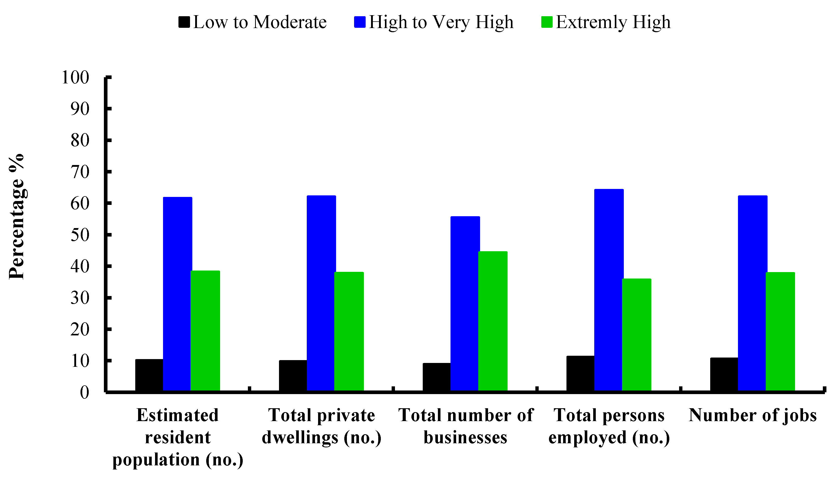
3.7. Flood Risk Evaluation

Floods are considered a complex natural disaster, causing a high number of lives lost and severe economic losses [94,95]. Across Australia, 1859 individually identified flood fatalities have been recorded for the period from 1900 to 2015 [96]. The highest number of these fatalities have been recorded in New South Wales [96]. In most cases (38.5%), victims died during their attempts to cross creeks, bridges, or roads in during floods while another 31.5% of the fatalities were in houses—the majority awaiting rescue or simply unaware of the flood [96].

In the present study, the geomorphic analysis highlighted the flood-susceptible areas in the Onkaparinga basin of south Australia. With the aim of identifying the flood hazard, the estimated resident population, total private dwellings, total number of businesses, total persons employed, and number of jobs were correlated with the identified susceptible zones (Figure 11). Results showed that out of the total human settlements in the Onkaparinga Basin, 55.88% are located in the highly susceptible sub-catchments, 27.60% are situated in moderately susceptible zones, while 16.52% are distributed in low and moderately susceptible areas. Most of the private dwellings are situated in the high-to-moderate susceptible zones (about 84% of the total private dwellings). Similarly, about 52.70% of the total number of businesses are found in the high-susceptible catchments, 31.09% in the moderately susceptible catchments, and 16.21% in the low-susceptible catchments. This indicates a significant widespread threat to the economy, environment, and community in the study area. The 2016 flood event caused damage to transport, power, and telecommunications infrastructure, with severe cost and disruption to the community. The event inundated homes, requiring some Old Noarlunga residents to evacuate, and it also damaged bridges, paths, and levee banks, which impacted 250 crop growers with estimated losses of AUD 66 m. In brief, flood susceptibility, presented in the above discussion, is an evaluation of where the future events may occur and to what extent the study area will be affected.

4. Conclusions

The GIS-based geomorphometric analysis of the Onkaparinga River Basin, South Australia are employed to identify the flood susceptibility and potential flood hazard zones. The remote sensing data (RS), including the Shuttle Radar Topographic Mission (SRTM) digital elevation model and Landsat images, are used to delineate 19 catchments in the Onkaparinga Basin. Based on the mathematical computation, 22 morphometric parameters are estimated, grouped into scale, shape, and relief, and ranked for flood susceptibility zones. The Onkaparinga River Basin was then classified into three flood vulnerability zones, namely, high to extremely high vulnerability (70–75), moderate-to-high vulnerability (65–70), and low-to-moderate vulnerability (60–65). By applying this ranking, Scott Creek, Western Branch, Biggs Flat, Chandlers Hill, and Echunga Creek have the lowest total score values, and thus represent a low-to-medium flooding susceptibility. Lenswood Creek, Mitchell Creek, Clarendon Weir, Cox Creek, Mount Bold Reservoir, Charleston, Upper Onkaparinga, Balhannah, and Hahndorf have intermediate score values, and are thus characterized by moderate-to-high flooding susceptibility, while Aldgate Creek, Lower Onkaparinga, Baker Gully, and Inverbrackie Creek have the highest overall score values and, consequently, represent the most dangerous areas with high flooding susceptibility. So, as the total score increases, the susceptibility of the catchments increase. In general, the eastern and northeastern areas, which are mostly covered by high topography, steep slopes, dominant metamorphic rocks with less permeability, less infiltration capacity, and greater runoff, have high flood potentiality, while the southwestern areas, which consist of gentle slopes, Quaternary unconsolidated sediments with high permeability, and high infiltration, have less flood potentiality. The results were also validated against the historical flood data and rainfall indices. A good correlation was found between the climate regime in terms of the precipitation concentration index (PCI) and rainfall anomaly index (RAI) and the flood susceptibility zones. Flood hazard analysis was undertaken further using the demographic data. The results indicated that 55.88% of the population are at risk of losing lives and property by flood events. Moreover, the present study proved that the implantation of the geomorphometric analysis can be used at different scales to assist the decision makers in understanding the spatial distribution of flood hazard and formulating flood mitigation strategies to reduce the negative impacts of future flooding on residents and infrastructure.

5. Limitation and Recommendations

This study provides a significant amount of information about susceptible flood zones in an important basin and the associated impacts with its devastating hazards on the population and economy. This study does, however, have some limitations. In the present study, relative flood risk and the ranking of flood susceptibility were determined, with a focus on assessing flood susceptibility at the watershed scale. The scale of the watershed or basin should be reduced to a microscale to have more benefit in the development of flood risk mitigation strategies by the local organizations responsible for watershed management. Other remote sensing data, such as synthetic aperture radar (SAR) images, could be efficiently used to support the observation and mapping of floods at this smaller scale. In addition, the simulation of flooding using hydrological dynamic modelling and/or analytical hierarchy process (AHP) can add more accuracy to susceptibility flood mapping.

References

1. Guha-Sapir, D.; Vos, F.; Below, R.; Ponserre, S. Annual Disaster Statistical Review 2011: The Numbers and Trends. 2012. Available online: https://mckellinstitute.org.au/wp-content/uploads/2022/09/The-Cost-of-Extreme-Weather-2022.pdf (accessed on 2 October 2022).
2. Leaning, J.; Guha-Sapir, D. Natural disasters, armed conflict, and public health. N. Engl. J. Med. 2013, 369, 1836–1842. [Google Scholar] [CrossRef] [PubMed]
3. Du, W.; FitzGerald, G.J.; Clark, M.; Hou, X.-Y. Health impacts of floods. Prehospital Disaster Med. 2010, 25, 265–272. [Google Scholar] [CrossRef] [PubMed]
4. Markantonis, V.; Meyer, V.; Lienhoop, N. Evaluation of the environmental impacts of extreme floods in the Evros River basin using Contingent Valuation Method. Nat. Hazards 2013, 69, 1535–1549. [Google Scholar] [CrossRef]
5. Lefebvre, M.; Reinhard, J. The Cost of extreme Weather “Building Resilience in the Face of Disaster”; The McKell Institute: Sydney, Australia, 2022; p. 32. [Google Scholar]
6. Hettiarachchi, S.; Wasko, C.; Sharma, A. Increase in flood risk resulting from climate change in a developed urban watershed–the role of storm temporal patterns. Hydrol. Earth Syst. Sci. 2018, 22, 2041–2056. [Google Scholar] [CrossRef] [Green Version]
7. Sharma, A.; Wasko, C.; Lettenmaier, D.P. If precipitation extremes are increasing, why aren’t floods? Water Resour. Res. 2018, 54, 8545–8551. [Google Scholar] [CrossRef]
8. Tehrany, M.S.; Jones, S.; Shabani, F. Identifying the essential flood conditioning factors for flood prone area mapping using machine learning techniques. Catena 2019, 175, 174–192. [Google Scholar] [CrossRef]
9. Sarkar, D.; Mondal, P. Flood vulnerability mapping using frequency ratio (FR) model: A case study on Kulik river basin, Indo-Bangladesh Barind region. Appl. Water Sci. 2019, 10, 17. [Google Scholar] [CrossRef] [Green Version]
10. Shehata, M.; Mizunaga, H. Flash flood risk assessment for Kyushu Island, Japan. Environ. Earth Sci. 2018, 77, 76. [Google Scholar] [CrossRef]
11. Creutin, J.D.; Borga, M.; Gruntfest, E.; Lutoff, C.; Zoccatelli, D.; Ruin, I. A space and time framework for analyzing human anticipation of flash floods. J. Hydrol. 2013, 482, 14–24. [Google Scholar] [CrossRef]
12. Creutin, J.D.; Borga, M. Radar hydrology modifies the monitoring of flash-flood hazard. Hydrol. Process. 2003, 17, 1453–1456. [Google Scholar] [CrossRef]
13. Borga, M.; Boscolo, P.; Zanon, F.; Sangati, M. Hydrometeorological analysis of the 29 August 2003 flash flood in the Eastern Italian Alps. J. Hydrometeorol. 2007, 8, 1049–1067. [Google Scholar] [CrossRef]
14. Canter, L.W.; Atkinson, S. Multiple uses of indicators and indices in cumulative effects assessment and management. Environ. Impact Assess. Rev. 2011, 31, 491–501. [Google Scholar] [CrossRef]
15. Korytny, L.M.; Kichigina, N.V. Geographical analysis of river floods and their causes in southern East Siberia. Hydrol. Sci. J. 2006, 51, 450–464. [Google Scholar] [CrossRef]
16. Mohamed, S.A.; El-Raey, M.E. Vulnerability assessment for flash floods using GIS spatial modeling and remotely sensed data in El-Arish City, North Sinai, Egypt. Nat. Hazards 2020, 102, 707–728. [Google Scholar] [CrossRef]
17. Bhattacharya, R.K.; Chatterjee, N.D.; Das, K. An integrated GIS approach to analyze the impact of land use change and land cover alteration on ground water potential level: A study in Kangsabati Basin, India. Groundw. Sustain. Dev. 2020, 11, 100399. [Google Scholar] [CrossRef]
18. Singh, S.; Dhote, P.R.; Thakur, P.K.; Chouksey, A.; Aggarwal, S. Identification of flash-floods-prone river reaches in Beas river basin using GIS-based multi-criteria technique: Validation using field and satellite observations. Nat. Hazards 2021, 105, 2431–2453. [Google Scholar] [CrossRef]
19. Bhat, M.S.; Alam, A.; Ahmad, S.; Farooq, H.; Ahmad, B. Flood hazard assessment of upper Jhelum basin using morphometric parameters. Environ. Earth Sci. 2019, 78, 54. [Google Scholar] [CrossRef]
20. Singh, O.; Kumar, D. Evaluating the influence of watershed characteristics on flood vulnerability of Markanda River basin in north-west India. Nat. Hazards 2019, 96, 247–268. [Google Scholar] [CrossRef]
21. Bajabaa, S.; Masoud, M.; Al-Amri, N. Flash flood hazard mapping based on quantitative hydrology, geomorphology and GIS techniques (case study of Wadi Al Lith, Saudi Arabia). Arab. J. Geosci. 2014, 7, 2469–2481. [Google Scholar] [CrossRef]
22. Abdel-Fattah, M.; Saber, M.; Kantoush, S.A.; Khalil, M.F.; Sumi, T.; Sefelnasr, A.M. A hydrological and geomorphometric approach to understanding the generation of wadi flash floods. Water 2017, 9, 553. [Google Scholar] [CrossRef]
23. Ahmed, A.; Hewa, G.; Alrajhi, A. Flood susceptibility mapping using a geomorphometric approach in South Australian basins. Nat. Hazards 2021, 106, 629–653. [Google Scholar] [CrossRef]
24. Sofi, M.S.; Rautela, K.S.; Bhat, S.U.; Rashid, I.; Kuniyal, J.C. Application of Geomorphometric Approach for the Estimation of Hydro-sedimentological Flows and Cation Weathering Rate: Towards Understanding the Sustainable Land Use Policy for the Sindh Basin, Kashmir Himalaya. Water Air Soil Pollut. 2021, 232, 280. [Google Scholar] [CrossRef]
25. Adnan, M.S.G.; Dewan, A.; Zannat, K.E.; Abdullah, A.Y.M. The use of watershed geomorphic data in flash flood susceptibility zoning: A case study of the Karnaphuli and Sangu river basins of Bangladesh. Nat. Hazards 2019, 99, 425–448. [Google Scholar] [CrossRef]
26. Costache, R.; Pham, Q.B.; Sharifi, E.; Linh, N.T.T.; Abba, S.I.; Vojtek, M.; Vojteková, J.; Nhi, P.T.T.; Khoi, D.N. Flash-flood susceptibility assessment using multi-criteria decision making and machine learning supported by remote sensing and GIS techniques. Remote Sens. 2020, 12, 106. [Google Scholar] [CrossRef] [Green Version]
27. Dano, U.L.; Balogun, A.-L.; Matori, A.-N.; Wan Yusouf, K.; Abubakar, I.R.; Said Mohamed, M.A.; Aina, Y.A.; Pradhan, B. Flood susceptibility mapping using GIS-based analytic network process: A case study of Perlis, Malaysia. Water 2019, 11, 615. [Google Scholar] [CrossRef] [Green Version]
28. Wang, Y.; Hong, H.; Chen, W.; Li, S.; Pamučar, D.; Gigović, L.; Drobnjak, S.; Tien Bui, D.; Duan, H. A hybrid GIS multi-criteria decision-making method for flood susceptibility mapping at Shangyou, China. Remote Sens. 2019, 11, 62. [Google Scholar] [CrossRef] [Green Version]
29. Avand, M.; Moradi, H. Using machine learning models, remote sensing, and GIS to investigate the effects of changing climates and land uses on flood probability. J. Hydrol. 2021, 595, 125663. [Google Scholar] [CrossRef]
30. Kabenge, M.; Elaru, J.; Wang, H.; Li, F. Characterizing flood hazard risk in data-scarce areas, using a remote sensing and GIS-based flood hazard index. Nat. Hazards 2017, 89, 1369–1387. [Google Scholar] [CrossRef]
31. Unduche, F.; Tolossa, H.; Senbeta, D.; Zhu, E. Evaluation of four hydrological models for operational flood forecasting in a Canadian Prairie watershed. Hydrol. Sci. J. 2018, 63, 1133–1149. [Google Scholar] [CrossRef] [Green Version]
32. Ghosh, A.; Kar, S.K. Application of analytical hierarchy process (AHP) for flood risk assessment: A case study in Malda district of West Bengal, India. Nat. Hazards 2018, 94, 349–368. [Google Scholar] [CrossRef]
33. Chakraborty, S.; Mukhopadhyay, S. Assessing flood risk using analytical hierarchy process (AHP) and geographical information system (GIS): Application in Coochbehar district of West Bengal, India. Nat. Hazards 2019, 99, 247–274. [Google Scholar] [CrossRef]
34. Vojtek, M.; Vojteková, J. Flood susceptibility mapping on a national scale in Slovakia using the analytical hierarchy process. Water 2019, 11, 364. [Google Scholar] [CrossRef] [Green Version]
35. Costache, R. Flash-flood Potential Index mapping using weights of evidence, decision Trees models and their novel hybrid integration. Stoch. Environ. Res. Risk Assess. 2019, 33, 1375–1402. [Google Scholar] [CrossRef]
36. Jaafari, A. LiDAR-supported prediction of slope failures using an integrated ensemble weights-of-evidence and analytical hierarchy process. Environ. Earth Sci. 2018, 77, 42. [Google Scholar] [CrossRef]
37. Tang, Z.; Zhang, H.; Yi, S.; Xiao, Y. Assessment of flood susceptible areas using spatially explicit, probabilistic multi-criteria decision analysis. J. Hydrol. 2018, 558, 144–158. [Google Scholar] [CrossRef]
38. Arabameri, A.; Rezaei, K.; Cerda, A.; Lombardo, L.; Rodrigo-Comino, J. GIS-based groundwater potential mapping in Shahroud plain, Iran. A comparison among statistical (bivariate and multivariate), data mining and MCDM approaches. Sci. Total Environ. 2019, 658, 160–177. [Google Scholar] [CrossRef] [PubMed]
39. Jabbari, A.; Bae, D.-H. Application of Artificial Neural Networks for accuracy enhancements of real-time flood forecasting in the Imjin basin. Water 2018, 10, 1626. [Google Scholar] [CrossRef] [Green Version]
40. Fang, Z.; Wang, Y.; Peng, L.; Hong, H. Predicting flood susceptibility using LSTM neural networks. J. Hydrol. 2021, 594, 125734. [Google Scholar] [CrossRef]
41. Shu, C.; Ouarda, T.B. Regional flood frequency analysis at ungauged sites using the adaptive neuro-fuzzy inference system. J. Hydrol. 2008, 349, 31–43. [Google Scholar] [CrossRef]
42. Termeh, S.V.R.; Kornejady, A.; Pourghasemi, H.R.; Keesstra, S. Flood susceptibility mapping using novel ensembles of adaptive neuro fuzzy inference system and metaheuristic algorithms. Sci. Total Environ. 2018, 615, 438–451. [Google Scholar] [CrossRef]
43. Nandi, A.; Mandal, A.; Wilson, M.; Smith, D. Flood hazard mapping in Jamaica using principal component analysis and logistic regression. Environ. Earth Sci. 2016, 75, 465. [Google Scholar] [CrossRef]
44. Johnson, F.; White, C.J.; van Dijk, A.; Ekstrom, M.; Evans, J.P.; Jakob, D.; Kiem, A.S.; Leonard, M.; Rouillard, A.; Westra, S.J.C.C. Natural hazards in Australia: Floods. Clim. Chang. 2016, 139, 21–35. [Google Scholar] [CrossRef] [Green Version]
45. Australian Bureau of Statistics. 2008 Year Book Australia No. 90; Australian Bureau of Statistics: Canberra, Australia, 2008.
46. Teoh, K.S. Estimating the Impact of Current Farm Dams Development on the Surface Water Resources of the Onkaparinga River Catchment. 2003. Available online: https://e-docs.geo-leo.de/handle/11858/00-1735-0000-0001-3370-3 (accessed on 2 October 2022).
47. Sturman, A.P.; Tapper, N.J. The Weather and Climate of Australia and New Zealand; Oxford University Press: Oxford, MO, USA, 1996. [Google Scholar]
48. Semenov, E.K.; Sokolikhina, E.V.; Sokolikhina, N.N. Vertical circulation in the tropical atmosphere during extreme El Niño-Southern Oscillation events. Russ. Meteorol. Hydrol. 2008, 33, 416–423. [Google Scholar] [CrossRef]
49. Dai, A.; Wigley, T.M.L. Global patterns of ENSO-induced precipitation. Geophys. Res. Lett. 2000, 27, 1283–1286. [Google Scholar] [CrossRef] [Green Version]
50. Preiss, W.V. The Adelaide Geosyncline: Late Proterozoic Stratigraphy, Sedimentation, Palaeontology and Tectonics; Department of Mines and Energy: Brasília, Brazil, 1987. [Google Scholar]
51. Zulfic, D.; Barnett, S.R.; Van den Akker, J. Mount Lofty Ranges groundwater assessment: Upper Onkaparinga catchment; Department of Water, Land and Biodiversity Conservation: Adelaide, Australia, 2003. [Google Scholar]
52. Preiss, W. The Adelaide Geosyncline of South Australia and its significance in Neoproterozoic continental reconstruction. Precambrian Res. 2000, 100, 21–63. [Google Scholar] [CrossRef]
53. May, R.I. Origin, Mineralogy and Diagenesis of Quaternary Sediments from the Noarlunga and Willunga Embayments, South Australia. Ph.D. Dissertation, Department of Soil Science, University of Adelaide, Adelaide, Australia, 1992. [Google Scholar]
54. Geoscience, A. SRTM-derived 1 Second Digital Elecation Models Version 1.0. 2011. Available online: https://ecat.ga.gov.au/geonetwork/srv/eng/catalog.search#/metadata/72759 (accessed on 2 September 2022).
55. Strahler, A.N. Quantitative analysis of watershed geomorphology. Eos Trans. Am. Geophys. Union 1957, 38, 913–920. [Google Scholar] [CrossRef] [Green Version]
56. Davis, J.C.; Sampson, R.J. Statistics and Data Analysis in Geology; Wiley: New York, NY, USA, 1986; Volume 646. [Google Scholar]
57. McCarthy, D.; Rogers, T.; Casperson, K. Floods in South Australia: 1836–2005; Bureau of Meteorology: Melbourne, Australia, 2006.
58. Oliver, J.E. Monthly precipitation distribution: A comparative index. Prof. Geogr. 1980, 32, 300–309. [Google Scholar] [CrossRef]
59. De Luis, M.; Gonzalez-Hidalgo, J.; Brunetti, M.; Longares, L.J.N.H.; Sciences, E.S. Precipitation concentration changes in Spain 1946–2005. Nat. Hazards Earth Syst. Sci. 2011, 11, 1259–1265. [Google Scholar] [CrossRef] [Green Version]
60. Van Rooy, M. A rainfall Anomally Index Independent of Time and Space. Notos 1965, 14, 43–48. [Google Scholar]
61. Horton, R.E. Erosional development of streams and their drainage basins; hydrophysical approach to quantitative morphology. Geol. Soc. Am. Bull. 1945, 56, 275–370. [Google Scholar] [CrossRef] [Green Version]
62. Schumm, S.A. Evolution of drainage systems and slopes in badlands at Perth Amboy, New Jersey. Geol. Soc. Am. Bull. 1956, 67, 597–646. [Google Scholar] [CrossRef]
63. Horton, R.E. Drainage-basin characteristics. Am. Geophys. Union 1932, 13, 350–361. [Google Scholar] [CrossRef]
64. Greenbaum, D. Review of Remote Sensing Applications to Groundwater Exploration in Basement and Regolith. 1985. Available online: https://nora.nerc.ac.uk/id/eprint/505150/1/WC_OG_85_1.pdf (accessed on 2 October 2022).
65. Miller, V.C. A Quantitative Geomorphic Study of Drainage Basin Characteristics in the Clinch Mountain Area Virginia and Tennessee; Columbia University: New York, NY, USA, 1953. [Google Scholar]
66. Hadley, R.F.; Schumm, S.A. Sediment sources and drainage basin characteristics in upper Cheyenne River basin. US Geol. Surv. Water-Supply Pap. 1961, 1531, 198. [Google Scholar]
67. Mesa, L.M. Morphometric analysis of a subtropical Andean basin (Tucuman, Argentina). Environ. Geol. 2006, 50, 1235–1242. [Google Scholar] [CrossRef]
68. Singh, N.; Singh, K.K. Geomorphological analysis and prioritization of sub-watersheds using Snyder’s synthetic unit hydrograph method. Appl. Water Sci. 2017, 7, 275–283. [Google Scholar] [CrossRef] [Green Version]
69. Sreedevi, P.; Owais, S.; Khan, H.; Ahmed, S. Morphometric analysis of a watershed of South India using SRTM data and GIS. J. Geol. Soc. India 2009, 73, 543–552. [Google Scholar] [CrossRef]
70. Sreedevi, P.; Subrahmanyam, K.; Ahmed, S. The significance of morphometric analysis for obtaining groundwater potential zones in a structurally controlled terrain. Environ. Geol. 2005, 47, 412–420. [Google Scholar] [CrossRef]
71. Reddy, G.O.; Maji, A.; Chary, G.; Srinivas, C.; Tiwary, P.; Gajbhiye, K. GIS and remote sensing applications in prioritization of river sub basins using morphometric and USLE parameters-a case study. Asian J. Geoinform. 2004, 4, 35–50. [Google Scholar]
72. Bhatt, S.; Ahmed, S. Morphometric analysis to determine floods in the Upper Krishna basin using Cartosat DEM. Geocarto Int. 2014, 29, 878–894. [Google Scholar] [CrossRef]
73. Pande, C.B.; Moharir, K. GIS based quantitative morphometric analysis and its consequences: A case study from Shanur River Basin, Maharashtra India. Appl. Water Sci. 2017, 7, 861–871. [Google Scholar] [CrossRef] [Green Version]
74. Chitra, C.; Alaguraja, P.; Ganeshkumari, K.; Yuvaraj, D.; Manivel, M. Watershed characteristics of Kundah sub basin using remote sensing and GIS techniques. Int. J. Geomat. Geosci. 2011, 2, 311. [Google Scholar]
75. Smith, K.G. Standards for grading texture of erosional topography. Am. J. Sci. 1950, 248, 655–668. [Google Scholar] [CrossRef]
76. Abdel-Lattif, A.; Sherief, Y. Morphometric analysis and flash floods of Wadi Sudr and Wadi Wardan, Gulf of Suez, Egypt: Using digital elevation model. Arab. J. Geosci. 2012, 5, 181–195. [Google Scholar] [CrossRef]
77. McCuen, R.H.; Wong, S.L.; Rawls, W.J. Estimating urban time of concentration. J. Hydraul. Eng. 1984, 110, 887–904. [Google Scholar] [CrossRef]
78. Thomas, J.; Joseph, S.; Thrivikramji, K.; Abe, G.; Kannan, N. Morphometrical analysis of two tropical mountain river basins of contrasting environmental settings, the southern Western Ghats, India. Environ. Earth Sci. 2012, 66, 2353–2366. [Google Scholar] [CrossRef]
79. Sklash, M.G.; Farvolden, R.N. The role of groundwater in storm runoff. J. Hydrol. 1979, 43, 45–65. [Google Scholar] [CrossRef]
80. Youssef, A.M.; Pradhan, B.; Hassan, A.M. Flash flood risk estimation along the St. Katherine road, southern Sinai, Egypt using GIS based morphometry and satellite imagery. Environ. Earth Sci. 2011, 62, 611–623. [Google Scholar] [CrossRef]
81. Altaf, F.; Meraj, G.; Romshoo, S.A. Morphometric analysis to infer hydrological behaviour of Lidder watershed, Western Himalaya, India. Geogr. J. 2013, 2013, 178021. [Google Scholar] [CrossRef] [Green Version]
82. Wentz, E.A. A shape definition for geographic applications based on edge, elongation, and perforation. Geogr. Anal. 2000, 32, 95–112. [Google Scholar] [CrossRef]
83. Roux, H.; Labat, D.; Garambois, P.-A.; Maubourguet, M.-M.; Chorda, J.; Dartus, D. A physically-based parsimonious hydrological model for flash floods in Mediterranean catchments. Nat. Hazards Earth Syst. Sci. 2011, 11, 2567–2582. [Google Scholar] [CrossRef] [Green Version]
84. Patton, P.C. Drainage basin morphometry and floods. In Flood Geomorphology; John Wiley & Sons: New York, NY, USA, 1988; pp. 51–64. [Google Scholar]
85. Ogarekpe, N.M.; Obio, E.A.; Tenebe, I.T.; Emenike, P.C.; Nnaji, C.C. Flood vulnerability assessment of the upper Cross River basin using morphometric analysis. Geomat. Nat. Hazards Risk 2020, 11, 1378–1403. [Google Scholar] [CrossRef]
86. Mahala, A. The significance of morphometric analysis to understand the hydrological and morphological characteristics in two different morpho-climatic settings. Appl. Water Sci. 2020, 10, 33. [Google Scholar] [CrossRef] [Green Version]
87. Patton, P.C.; Baker, V.R. Morphometry and floods in small drainage basins subject to diverse hydrogeomorphic controls. Water Resour. Res. 1976, 12, 941–952. [Google Scholar] [CrossRef] [Green Version]
88. Masoud, M.H. Geoinformatics application for assessing the morphometric characteristics’ effect on hydrological response at watershed (case study of Wadi Qanunah, Saudi Arabia). Arab. J. Geosci. 2016, 9, 280. [Google Scholar] [CrossRef]
89. Keesstra, S. Impact of natural reforestation on floodplain sedimentation in the Dragonja basin, SW Slovenia. Earth Surf. Process. Landf. J. Br. Geomorphol. Res. Group 2007, 32, 49–65. [Google Scholar] [CrossRef]
90. Norman, L.M.; Huth, H.; Levick, L.; Shea Burns, I.; Phillip Guertin, D.; Lara-Valencia, F.; Semmens, D. Flood hazard awareness and hydrologic modelling at Ambos Nogales, United States–Mexico border. J. Flood Risk Manag. 2010, 3, 151–165. [Google Scholar] [CrossRef]
91. Tehrany, M.S.; Pradhan, B.; Mansor, S.; Ahmad, N. Flood susceptibility assessment using GIS-based support vector machine model with different kernel types. Catena 2015, 125, 91–101. [Google Scholar] [CrossRef]
92. Jonkman, S.N. Global perspectives on loss of human life caused by floods. Nat. Hazards 2005, 34, 151–175. [Google Scholar] [CrossRef]
93. Khan, K.A.; Zaman, K.; Shoukry, A.M.; Sharkawy, A.; Gani, S.; Ahmad, J.; Khan, A.; Hishan, S.S. Natural disasters and economic losses: Controlling external migration, energy and environmental resources, water demand, and financial development for global prosperity. Environ. Sci. Pollut. Res. 2019, 26, 14287–14299. [Google Scholar] [CrossRef]
94. Haynes, K.; Coates, L.; van den Honert, R.; Gissing, A.; Bird, D.; de Oliveira, F.D.; D’Arcy, R.; Smith, C.; Radford, D.J. Exploring the circumstances surrounding flood fatalities in Australia—1900–2015 and the implications for policy and practice. Environ. Sci. Policy 2017, 76, 165–176. [Google Scholar] [CrossRef]
95. Coates, L. Flood fatalities in Australia, 1788-1996. Aust. Geogr. 1999, 30, 391–408. [Google Scholar] [CrossRef]
96. FitzGerald, G.; Du, W.; Jamal, A.; Clark, M.; Hou, X.Y. Flood fatalities in contemporary Australia (1997–2008). Emerg. Med. Australas. 2010, 22, 180–186. [Google Scholar] [CrossRef] [PubMed]
Figure 1. Location of the Onkaparinga River Basin.
Sustainability 14 16270 g001
Figure 2. Geologic and structural features of the Onkaparinga River Basin.
Sustainability 14 16270 g002
Figure 3. Methodology applied to identify the flood susceptibility zones flow chart.
Sustainability 14 16270 g003
Figure 4. The location of the selected rainfall stations in the study area.
Sustainability 14 16270 g004
Figure 5. Flash flood susceptibility ranking in relation to stream characteristics of the Onkaparinga River Basin.
Sustainability 14 16270 g005
Figure 6. Flood susceptibility ranking in relation to scale characteristics of the Onkaparinga River Basin.
Sustainability 14 16270 g006
Figure 7. Flood susceptibility ranking in relation to shape characteristics of the Onkaparinga River Basin.
Sustainability 14 16270 g007
Figure 8. Flash flood susceptibility ranking in relation to relief characteristics of the Onkaparinga River Basin.
Sustainability 14 16270 g008
Figure 9. Flood susceptibility map based on the ranking of the morphometric analysis of the Onkaparinga River Basin.
Sustainability 14 16270 g009
Figure 10. Validation of the susceptibility using historical floods (a), rainfall indices (b,c).
Sustainability 14 16270 g010
Figure 11. Flood susceptibility versus demographic data to identify the flood hazard.
Sustainability 14 16270 g011