Abstract
The scientific prediction of energy consumption plays an essential role in grasping trends in energy consumption and optimizing energy structures. Energy consumption will be affected by many factors. In this paper, in order to improve the accuracy of the prediction model, the grey correlation analysis method is used to analyze the relevant factors. First, the factor with the largest correlation degree is selected, and then a new grey multivariable convolution prediction model with dual orders is established. Different fractional orders are used to accumulate the target data sequence and the influencing-factor data sequence, and the model is optimized by particle swarm optimization algorithm. The model is used to fit and test the energy consumption of Shanghai, Guizhou and Shandong provinces in China from 2011 to 2020 compared with other multivariable grey prediction models. Experimental results with the MAPE and RMSPE measurements show that our improved model is reasonable and effective in energy consumption prediction. At the same time, the model is applied to forecast the energy consumption of the three regions from 2021 to 2025, providing reliable information for future energy distribution.
1. Introduction
With the fast development of the social economy and industry, the energy consumed by humankind is also growing. Currently, energy is the indispensable material basis for human survival and development, and it is also important for supporting the normal operation of society and economy. At present, China is the world’s second largest economy. Because of its rapidly developing economy, China’s energy consumption is also increasing year by year. However, the world’s resources are not unlimited. Excessive energy consumption will cause a certain degree of damage to the global ecological environment and is not conducive to the sustainable development of all countries. In order to make a more rational use of energy, energy consumption prediction is particularly important. Through the scientific prediction of energy consumption, we can predict future trends in energy use, providing the basis for relevant departments to formulate reasonable energy consumption plans, optimize energy structures, and promote the realization of social, economic and ecological sustainable development.
Recently, many domestic and foreign scholars have adopted different models and methods to study different kinds of energy consumption. Chaturvedi et al. [1] compared the performances of Indian’s Central Energy Authority’s (CEA) existing trend-based model, SARIMA, LSTM RNN and Facebook prophet in predicting monthly total energy demand and peak energy demand of India. Peng et al. [2] proposed an optimized long short-term memory-based model and applied it to the prediction of energy consumption. Rick et al. [3] proposed a deep learning approach based on LSTM, CNN and an auto-encoder to predict data with different time series lengths. Jin et al. [4] combined singular spectrum analysis (SSA) and parallel long- and short-term memory (PLSTM) neural networks to form a new hybrid artificial intelligence prediction model and predicted the power consumption of five families in the UK. Somu et al. [5] presented an energy consumption forecasting model based on long short-term memory networks and improved a sine cosine optimization algorithm to accurately predict building energy consumption, including the energy consumption of the teaching building in Indian Institute of Technology. Kazemzadeh et al. [6] proposed a hybrid forecasting method that combined the auto-regressive integrated moving average (ARIMA), an artificial neural network (ANN) and the proposed support vector regression technique, and used this method to forecast the annual peak load and total energy demand of Iran’s national electric energy system. Adedeji et al. [7] used a non-linear autoregressive neural network (NARNET) to predict the energy consumption of a university in South Africa. Zeng et al. [8] first identified 17 factors that affect the structure of Chinese energy consumption. On this basis, they used a copula function to develop a multi-factor dynamic support vector machine model to predict the advanced index of China’s energy consumption structure in the future. Hu et al. [9] developed a stacked hierarchy of reservoirs (DeepESN) for forecasting energy consumption and wind power generation by introducing the deep learning framework into the basic echo state network. Bedi et al. [10] proposed a memory network prediction model based on decomposition and automatic encoder integration, which can achieve an accurate prediction of power demand. These prediction models mentioned above are deep learning models and time series methods that need a large quantity of data for training to obtain more accurate prediction results.
However, in practice, energy consumption statistics are often small data samples. When the amount of sample data is not enough, the deep learning model loses its application value. The grey prediction model can play an important role because it requires fewer data samples. The grey prediction model is a key component of the grey system theory proposed by Professor Deng, which has wide applicability to the prediction problems of small samples, a lack of information and uncertainty [11]. Therefore, many scholars usually use a grey prediction model to solve the problem of energy prediction with less data.
Xiong et al. [12] proposed a new incomplete gamma grey forecasting model based on fractional-order accumulation and used this model to simulate and predict natural gas consumption in the Asia–Pacific region from 2008 to 2018. Tong et al. [13] used an extrapolation method to extend the background value of the GM (1,1) model, optimized the model with a simulated annealing algorithm, and applied the model to forecast the coal consumption of China, India and the United States in the next five years. Ding et al. [14] established an optimized structure-adaptative grey model to predict the nuclear energy consumption of China and America. Ma et al. [15] proposed a new fractional time-delayed grey model, which is optimized by the Grey Wolf Optimizer, and applied the model to forecast the coal and natural gas consumption in Chongqing. Wu et al. [16] combined fractional-order accumulation and a grey multivariable convolution model and established an FGMC (1,N) model that was used to forecast the power consumption of Shandong Province. Liu et al. [17] proposed an optimized nonlinear grey Bernoulli prediction model with weighted fractional accumulation generation operation and used five optimization algorithms to optimize the model’s parameters to predict the natural gas production of Germany, Italy, Canada and China. Wang et al. [18] introduced adjacent accumulation into the grey multivariable convolution model and established the AGMC (1,N) model to predict the energy consumption of 13 provinces (cities) in seven regions of China. Li et al. [19] selected a genetic algorithm to optimize the background value and established a new nonlinear multivariable Verhulst model to predict China’s oil consumption. Duan et al. [20] used a novel multivariable Verhulst grey model (MVGM (1,N)) to predict the coal consumption of the Inner Mongolia and Gansu provinces in China. Zhao et al. [21] studied the prediction of non-renewable energy consumption in the Asia–Pacific Economic Cooperation countries by using the adjacent accumulation discrete grey model. Chen et al. [22] proposed a modeling method based on a grey prediction model and cloud model to predict the energy consumption of Shanghai, Zhejiang, Jiangsu and Anhui provinces. Zhou et al. [23] established a discrete grey seasonal model by cycle accumulation generation and predicted monthly industrial electricity consumption and quarterly natural gas consumption. Zhou et al. [24] proposed a new optimized fractional grey Holt–Winters model (NOFGHW) and applied it to the prediction of monthly crude oil production and quarterly industrial electricity consumption. Cheng et al. [25] used an improved GM (1,N) model to simulate and predict China’s clean energy consumption. Zhang et al. [26] established a new incomplete gamma grey model (IGGM) to predict solar energy consumption in Japan. Wu et al. [27] proposed a novel nonlinear grey Bernoulli model with fractional-order accumulation (FANGBM (1,1) model) to predict China’s renewable energy consumption from 2016 to 2020. Wang et al. [28] proposed a new fractional time-delayed grey Bernoulli model for data with scarcity, complexity and nonlinear characteristics, and predicted renewable energy, crude oil and fossil fuels usage. Liu et al. [29] established a discrete fractional grey model with a time power term and made a reliable prediction of China’s natural gas consumption. Wang et al. [30] proposed a new fractional-order grey model FENBGM (1,1) to forecast China’s oil consumption.
From the above research, we can see that scholars have improved the prediction accuracy of the grey prediction model from different aspects, such as optimizing the background value of the model, proposing new accumulation operators, etc. Although scholars have made great progress in energy consumption prediction at present, there are still problems, such as single factors affecting energy consumption, model improvements mainly focusing on background value optimization, a lack of sequence smoothness improvements, etc. These problems restrict improvements in model prediction accuracy. Therefore, in order to make the prediction of energy consumption more scientific and reasonable, considering that energy consumption is affected by many factors, such as economic development, national policies, population and the living standards of residents, a new grey multivariable prediction model is proposed in this paper, which can provide an effective reference for the government to formulate reasonable energy use policies. Tien (2005) [31] improved the basic GM (1,N) model and proposed a grey multivariable convolution model (GMC (1,N)), which effectively improved the prediction accuracy. The basic GMC (1,N) model uses first-order accumulation to generate sequences, which cannot make full use of old and new information and has certain limitations. In order to predict energy consumption more accurately, this paper introduces the different-order accumulation generation sequence proposed by Yin [32] into the GMC (1,N) model and then constructs a new dual-order multivariable grey convolution prediction model (FGMC (1,N,2r)). At the same time, a particle swarm optimization algorithm is selected to optimize the two fractional orders, which further increases the prediction accuracy of the model.
The main contributions of this paper are as follows:
- (1)
- In order to obtain the objective factors affecting energy consumption and establish a reasonable grey multivariable model, six factors affecting energy consumption are selected for grey relation analysis, from which the impact index with the largest correlation degree is selected;
- (2)
- On the basis of combining the different-order accumulation method and the grey multivariable convolution model, the grey multivariable convolution model based on different fractional-order accumulation is established. Different fractional orders are used to accumulate the target sequence and the influencing factor sequence, which can make full use of the information of different data sequences and reflect the influence of influencing factors on the change trend of the target sequence. Additionally, a particle swarm optimization algorithm is used to optimize fractional orders and . The model is used to fit, test and forecast the energy consumption of some provinces (cities) in China, which verifies the effectiveness of the model.
The other main parts of this paper are as follows: In Section 2, the relevant methods involved in the paper are introduced. In Section 3, the grey multivariable convolution model based on different fractional-order accumulation is proposed and the optimization method of the model parameters and model inspection index are given. In Section 4, we compare and discuss the energy consumption prediction results of the three provinces and use the model to simulate and test the energy consumption of other provinces (cities). In Section 5, the conclusions and suggestions of this paper are drawn.
2. Related Methods
2.1. Grey Relation Analysis
The main idea of grey relation analysis is to transform the system’s data series of influencing factors into sequence polylines and then construct a model to measure the degree of relevance on the basis of the geometric characteristics of the polylines. The more similar the geometric shape of the broken line is, the greater the relational degree between the corresponding sequences, and vice versa. Different from the traditional mathematical statistics method, it has no strict requirements on the amount and law of data, and the amount of calculation is small. Therefore, it is scientific and reasonable to choose the grey relation analysis method to analyze the impact of economic conditions, population, environment and other factors on energy consumption. In this paper, Deng’s grey correlation degree [33] is used to calculate the correlation degree between relevant factors and energy consumption. The specific calculation steps are as described below.
Step 1: Assuming that is the sequence of dependent variable (target variable) and is the sequence of independent variables (influencing factors).
Step 2: The sequence and sequence are processed dimensionless, and the initial value images of each sequence are obtained by Equations (1) and (2).
Step 3: Use the Equation (3) to calculate the absolute difference sequence of and .
Step 4: Finding that the maximum value of is and the minimum value of is .
Step 5: Use the Equation (4) to calculate the correlation coefficient and use Equation (5) to calculate Deng’s grey correlation degree.
2.2. Particle Swarm Optimization
Particle swarm optimization (PSO) is a classical swarm intelligence algorithm, which originates from research on the predatory behavior of birds. The core of the algorithm is to find the optimal solution of the problem by using cooperation and information sharing among individuals in the group [34]. The specific description of the particle swarm optimization algorithm is as follows: First, a group of particles is initialized, assuming that there are particles in the search space, where the position of the particle in the space is expressed as and the velocity is expressed as . We can obtain its fitness value by substituting the position of each particle into the objective function and determine the quality of the position according to the fitness value. The historical optimal position of the particle is expressed as and the historical optimal position of the global particle is . The velocity and position of each generation of particles can be iteratively calculated according to Equations (6) and (7).
Among them, is the inertia factor, and its value is non-negative. The bigger the value of is, the more the particles focus on the global search, and the smaller the value of is, the more the particles focus on the local search. and are the learning factors and constants, which determine the maximum step size of particles moving to the individual optimal position and the global optimal position. and are two random numbers in the range of [0, 1], which are used to enhance the randomness of the search.
3. FGMC (1,N,2r) Model
3.1. Establishment of the Model
The fractional order is one of the major factors that influence the results of the fractional grey multivariable prediction model. In many existing grey multivariable prediction models, the target sequence and influencing factor sequence are accumulated by the same order, and different data sequences often have different characteristics. Using the same accumulation operator ignores the differences between data sequences. Therefore, in this paper, the different fractional orders that are used to accumulate the target sequence and influencing factor sequence are introduced into the GMC (1,N) model to construct a FGMC (1,N,2r) model. The modeling process is as shown below.
Step 1: Assume the target sequence is and the influencing factor sequence is .
Step 2: is the fractional-order-accumulated generation of the target sequence of by using Equation (8). is the fractional-order-accumulated generation of the influencing factor sequence of by using Equation (9).
Step 3: The convolution grey model of double fractional orders can be established as , where are parameters, which can be solved by the least square method according to Equation (10).
where,
Step 4: The time response function is obtained as Equation (11).
where .
Step 5: The final prediction sequence is obtained by Equation (12).
In order to more intuitively represent the FGMC (1,N,2r) model, the process of using the model for prediction is shown in a flowchart, as shown in Figure 1.
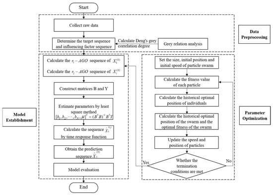
Figure 1.
The prediction process of FGMC (1,N,2r) model.
3.2. Parameter Optimization
An accumulation generation operator is an approach that makes a grey system turn from grey to white by using data mining and preprocessing technology. For the grey convolution multivariable prediction model based on different fractional-order accumulations, the orders and are important parameters that affect the original data preprocessing effect and model performance and act on the target sequence and the influencing factor sequence, respectively. The values of these two parameters have a decisive effect on the accuracy of the model, and the prediction accuracy of the model will change with their changes. Therefore, we select a particle swarm optimization algorithm to find the optimal value of the parameters, so as to improve the prediction accuracy and reduce the prediction error of the model. This optimization problem can be expressed by Equation (13).
The objective of the optimization problem is to find a set of parameters to minimize the MAPE value of the model. The constraints include the value range of the two parameter values and the relevant formulas involved in the modeling process of the model.
3.3. Model Evaluation Index
To verify different prediction models’ precision more reasonably, we choose three evaluation indexes, namely the absolute percentage error (APE), average absolute percentage error (MAPE) and root mean square percentage error (RMSPE), to evaluate the prediction accuracy of the model. The specific equations are shown in Equations (14)–(16). The accuracy tested by MAPE is shown in Table 1.

Table 1.
The accuracy of the model tested by MAPE.
4. Model Application
In order to improve energy efficiency and push forward the construction of a modern energy system, relevant policies focusing on green and low-carbon energy development have been formulated in all regions and provinces of China. In the process of promoting green energy consumption, the analysis and prediction of energy consumption in recent years is an essential step. Therefore, we selected Shanghai, Guizhou and Shandong because the development levels of these three regions are different and representative. The development level of Shanghai has basically reached the level of developed countries, the development level of Shandong is basically at the level of developing countries, and the development level of Guizhou is slightly lower than that of Shandong. The geographical locations of these three regions are shown in Figure 2. Then, we used the model proposed in this paper to fit and test the energy consumption of these three regions to forecast their energy consumption in the next few years.
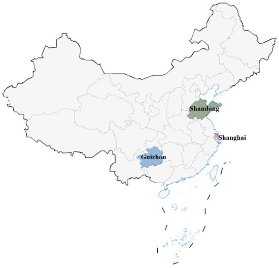
Figure 2.
Geographical distribution map of the study provinces.
4.1. Experimental Data Collections
Table 2 shows the total energy consumption data of Shanghai, Guizhou and Shandong from 2011 to 2020 that are used in this study. The energy consumption in Shanghai accounts for 2.51% of China’s energy consumption, that in Guizhou Province accounts for 2.04%, and that in Shandong Province accounts for 8.51% [35]. The data of the first eight years are used for model construction, and the data of the second two years are used for model testing.
Table 2.
Energy consumption of provinces (cities) during 2011–2020 (unit:10000 tce).
According to the relevant literature, six factors that affect energy consumption are preliminarily selected in this paper, namely the added value of the primary industry, the added value of the secondary industry, the added value of the tertiary industry, the total population, the urban per capita disposable income, and the rural per capita disposable income. The added value of the three major industries constitutes GDP, which reflects the economic condition of the province. Economic development is an important factor affecting energy consumption, and rapid economic development promotes the growth of energy consumption. Population also affects energy consumption. The increase in population means the increase in demand for various resources and, accordingly, energy consumption will also increase. In addition, urban per capita disposable income and rural per capita disposable income are the main indicators to reflect the living standards of residents. The growth in the living standards of residents will increase the consumption levels of high-quality energy, such as gasoline, electricity and natural gas, thus affecting energy consumption. On this basis, we use the grey correlation analysis method to select the factors most related to energy consumption for modeling.
All data are from the statistical yearbooks of all provinces (cities) and the official website of the National Bureau of Statistics (http://www.stats.gov.cn/ accessed on 6 July 2022). The statistical official website of each province (city) and their corresponding statistical yearbook can be accessed:
4.2. Model Comparison and Analysis
4.2.1. Energy Consumption in Shanghai
The data series of energy consumption is the target sequence, which is recorded as . The data series of the added value of the primary industry, the added value of the secondary industry, the added value of the tertiary industry, the total population, the urban per capita disposable income and the rural per capita disposable income are the influencing factor sequences, which are recorded as ,respectively. According to the calculation formula in Section 2.1, the grey correlation degrees between the energy consumption of Shanghai and the six influencing factors are calculated. The calculated results are shown in Table 3.
Table 3.
Grey correlation degree results of Shanghai.
It can be seen from Table 3 that the total population is the most significant factor affecting Shanghai’s energy consumption, with a correlation value of 0.9705. Therefore, on this basis, the FGMC (1,2,2r) model is built, and the PSO algorithm is used to optimize the values of the two fractional orders. Meanwhile, in order to better reflect the effectiveness and accuracy of the new model, the model is compared with four models, including the GM (1,N) model, GMC (1,N) model [24] optimized AGMC (1,N) model [18] and optimized FGMC (1,N) model [16]. The data sizes used in the five models involved in the comparison are identical, and a PSO algorithm is used to optimize the parameters of the models that need to be optimized.
Table 4 shows the modeling and testing results of energy consumption in Shanghai from 2011 to 2020 and gives the parameter values of each model after optimization. It can be seen from Table 4 that in the modeling stage, the MAPE of the five grey prediction models are 6.32%, 0.85%, 0.85%, 0.85%, and 0.40%, and the RMSPE are 8.16%, 1.09%, 1.27%, 1.27% and 0.49%. In the testing stage, the MAPE of the five models are 2.71%, 3.77%, 3.80%, 3.27% and 2.40%, and the RMSPE are 3.19%, 5.27%, 5.17%, 4.15% and 2.45%. From the two evaluation indexes, the grey multivariable convolution model based on different fractional orders presented in this paper has good results in modeling and testing and meets the model accuracy requirements, indicating that the model is excellent. In order to more clearly show the fitting and prediction effects of each model, the result comparison diagram is shown in Figure 3.
Table 4.
Modeling and testing results of energy consumption in Shanghai.
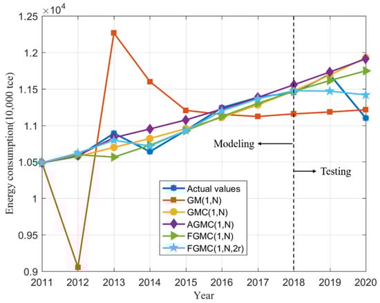
Figure 3.
Comparison of prediction results of energy consumption in Shanghai.
From the above analysis, we can see that the new model has a high prediction accuracy. Additionally, we can use this model to predict the energy consumption of Shanghai from 2021 to 2025. Meanwhile, the optimized FGM (1,1) model is used to predict the sequence of influencing factors. The final results are shown in Table 5. Table 5 shows that in the next five years, the energy consumption of Shanghai will follow a downward trend, which may be related to the slower growth rate of the population.
Table 5.
Forecasting results of energy consumption from 2021 to 2025 in Shanghai.
4.2.2. Energy Consumption in Guizhou
In the modeling and testing of energy consumption in Guizhou Province, the grey relation analysis method is also used to calculate the grey correlation degrees between energy consumption and the six influencing factors. The results are shown in Table 6. According to Table 6, the grey correlation degree between energy consumption and population in Guizhou Province is the largest, which is 0.8641. Therefore, the FGMC (1,2,2r) model is established with population as the influencing factor sequence, which is compared with the results of the other four grey models. The results are shown in Table 7 and the prediction results are shown in Figure 4.
Table 6.
Grey correlation degree results of Guizhou.
Table 7.
Modeling and testing results of energy consumption in Guizhou.
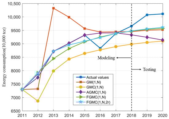
Figure 4.
Comparison of prediction results of energy consumption in Guizhou.
Table 7 shows that in the modeling stage, the MAPE of the five grey prediction models are 6.94%, 6.83%, 1.68%, 2.16% and 1.40%, and the RMSPE are 8.99%, 7.61%, 2.82%, 2.61% and 2.07%. In the testing stage, the MAPE of the five models are 5.76%, 10.09%, 8.96%, 5.35% and 5.07%, and the RMSPE are 5.76%, 10.09%, 8.98%, 5.35% and 5.07%. In the modeling stage and the testing stage, the MAPE and RMSPE of the proposed model are the smallest of the five models, which shows that this model is superior to other models.
In addition, the FGMC (1,2,2r) model is used to continuously forecast the energy consumption of Guizhou Province from 2021 to 2025. The results are shown in Table 8. The results reflect that the energy consumption of Guizhou Province generally presents an upward trend. As population is the most influential factor on the energy consumption of Guizhou Province, the energy consumption of Guizhou Province will also increase as the population increasing. However, the increasing trend is relatively gentle and there will be no excessive consumption of energy, which is of great significance for achieving sustainable development.
Table 8.
Forecasting results of energy consumption from 2021 to 2025 in Guizhou.
4.2.3. Energy Consumption in Shandong
Similarly, when studying the energy consumption of Shandong Province, the grey correlation degrees between the energy consumption and the six influencing factors are calculated first, and the results are shown in Table 9. Table 9 shows that the added value of the primary industry has the greatest correlation with the energy consumption of Shandong Province, with a value of 0.9420. Therefore, taking the added value of the primary industry as the influencing factor sequence, the five grey models are established, and Table 10 and Figure 5 are obtained. Compared with other models, the new model has better performance in fitting and predicting the trends of data, and some data points can almost coincide with the actual value.
Table 9.
Grey correlation degree results of Shandong.
Table 10.
Modeling and testing results of energy consumption in Shandong.
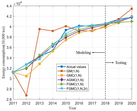
Figure 5.
Comparison of prediction results of energy consumption in Shandong.
In order to analyze the development trend of energy consumption in Shandong Province in the next few years, we apply the FGMC (1,2,2r) model to predict the energy consumption of Shandong Province from 2021 to 2025. The results are shown in Table 11. According to the prediction results, the energy consumption of Shandong Province generally presents a downward trend. Shandong is a large agricultural province, and the added value of the primary industry has the greatest impact on energy consumption. In the future, the energy consumption of Shandong Province will be inversely proportional to the added value of the primary industry, probably because Shandong Province has carried out a green and low-carbon transformation of its primary industry, which has improved its energy utilization efficiency.
Table 11.
Forecasting results of energy consumption from 2021 to 2025 in Shandong.
After analyzing and predicting the energy consumption of the three regions, we can draw the following conclusions:
- (1)
- Compared with other grey models, the FGMC (1,N,2r) model developed in this paper is more accurate in its predictions;
- (2)
- The new model has better prediction performance after parameter optimization;
- (3)
- The new model can make up for the shortcomings of other models in predicting energy consumption.
4.3. Further Discussion
The FGMC (1,N,2r) model is applied to fit and test the energy consumption of other provinces (cities) in China so as to achieve the purpose of testing the role of the new model in the prediction of energy consumption. The model parameter values of provinces (cities) are shown in Table 12. The results are shown in Table 13 and Table 14.
Table 12.
Model parameter values of provinces (cities).
Table 13.
Modeling and testing results of energy consumption in Zhejiang, Hebei and Chongqing.
Table 14.
Modeling and testing results of energy consumption in Jiangxi, Shanxi and Jiangsu.
From these data, this model has produced good results in the prediction of energy consumption in these six regions. In the modeling process from 2011 to 2018, all MAPE values are less than 1%. In the testing process from 2019 to 2020, the MAPE values are also controlled below 4%. When the model effect is good, the MAPE value can reach 0.17%.
In addition, we found that the influencing factors of each region are different, and the correlation between the influence factors and energy consumption is also different, which is one of the reasons for the model’s different prediction accuracies. However, in general, according to the accuracy of the model tested by MAPE given in Section 3.3 (see Table 1), the newly proposed model is excellent in the prediction of energy consumption, and its prediction performance indicators exceed the existing latest methods.
The development trends in energy consumption in China’s provinces (cities) are different; therefore, the governments and energy departments in different regions will need to take different measures. An accurate prediction of energy consumption can provide useful information for decision makers, help them formulate appropriate policies according to local conditions, and promote the optimization of energy structure. It has important practical significance.
5. Conclusions and the Future Work
To accurately predict energy consumption in different regions, a novel grey multivariable convolution prediction model based on different fractional-order accumulation is proposed. The new grey model uses different fractional orders to accumulate the target sequence and the influencing factor sequence, fully mining the information of different data sequences, and effectively combines the fractional-order accumulation and the grey multivariable convolution model. The main conclusions of this study are as follows:
- (1)
- The novel model is used to forecast the energy consumption of Shanghai, Guizhou and Shandong provinces. Compared with the simulation results of different grey models, the proposed grey multivariable convolution prediction model based on different fractional-order accumulation has higher prediction accuracy than the other grey multivariable prediction models, including the GM (1,N) model, GMC (1,N) model, AGMC (1,N) model and FGMC (1,N) model. From the two measurements of MAPE and RMSPE, the new model has the lowest MAPE and RMSPE values, making it superior to the other models;
- (2)
- Different fractional orders are used to accumulate the target sequence and the influencing factor sequence, which makes full use of the information of the data sequence with different characteristics. Furthermore, the optimized fractional-order and also greatly improve the prediction accuracy of the model;
- (3)
- The new model is a successful optimization of the grey multivariable convolution prediction model. It has a good performance in predicting energy consumption and it also provides a certain reference for other energy prediction problems.
Moreover, the limits of the study are as follows:
- (1)
- Grey relation analysis is applied to find out the most influential factors on energy consumption, and only one influencing factor is used to establish a grey multivariable model. In the future, more influencing factors can be considered to establish the model, which may lead to more accurate prediction results;
- (2)
- In this paper, a particle swarm optimization algorithm is used to optimize the parameters of the model. In the future, other optimization algorithms can be considered for optimization, and other parameters of the model can also be considered for optimization, so as to improve the prediction accuracy of the model;
- (3)
- The energy consumption data of 2020 is used and the impact of COVID-19 on energy consumption is temporarily ignored. This may be an important research direction in the future.
Author Contributions
Conceptualization, Y.S. and F.Z.; investigation, Y.S.; methodology, Y.S.; software, Y.S.; supervision, Y.S. and F.Z.; validation, Y.S.; writing—original draft, Y.S.; writing—review and editing, Y.S. and F.Z. All authors have read and agreed to the published version of the manuscript.
Funding
This research received no external funding.
Conflicts of Interest
The authors declare that they have no known competing financial interests or personal relationships that could have appeared to influence the work reported in this paper.
References
- Chaturvedi, S.; Rajasekar, E.; Natarajan, S.; McCullen, N. A comparative assessment of SARIMA, LSTM RNN and Fb Prophet models to forecast total and peak monthly energy demand for India. Energy Policy 2022, 168, 113097. [Google Scholar] [CrossRef]
- Peng, L.; Wang, L.; Xia, D.; Gao, Q. Effective energy consumption forecasting using empirical wavelet transform and long short-term memory. Energy 2022, 238, 121756. [Google Scholar] [CrossRef]
- Rick, R.; Berton, R. Energy forecasting model based on CNN-LSTM-AE for many time series with unequal lengths. Eng. Appl. Artif. Intell. 2022, 113, 104998. [Google Scholar] [CrossRef]
- Jin, N.; Yang, F.; Mo, Y.; Zeng, Y.; Zhou, X.; Yan, K.; Ma, X. Highly accurate energy consumption forecasting model based on parallel LSTM neural networks. Adv. Eng. Inform. 2022, 51, 101442. [Google Scholar] [CrossRef]
- Somu, N.; Raman, G.M.R.; Ramamritham, K. A hybrid model for building energy consumption forecasting using long short term memory networks. Appl. Energy 2020, 261, 114131. [Google Scholar] [CrossRef]
- Kazemzadeh, M.R.; Amjadian, A.; Amraee, T. A hybrid data mining driven algorithm for long term electric peak load and energy demand forecasting. Energy 2020, 204, 117948. [Google Scholar] [CrossRef]
- Adedeji, P.A.; Akinlabi, S.; Ajayi, O.; Madushele, N. Non-linear autoregressive neural network (NARNET) with SSA filtering for a university energy consumption forecast. Procedia Manuf. 2019, 33, 176–183. [Google Scholar] [CrossRef]
- Zeng, S.; Su, B.; Zhang, M.; Gao, Y.; Liu, J.; Luo, S.; Tao, Q. Analysis and forecast of China’s energy consumption structure. Energy Policy 2021, 159, 112630. [Google Scholar] [CrossRef]
- Hu, H.; Wang, L.; Lv, S. Forecasting energy consumption and wind power generation using deep echo state network. Renew. Energy 2020, 154, 598–613. [Google Scholar] [CrossRef]
- Bedi, J.; Toshniwal, D. Energy load time-series forecast using decomposition and autoencoder integrated memory network. Appl. Soft Comput. 2020, 93, 106390. [Google Scholar] [CrossRef]
- Deng, J.L. Control problem of grey system. Syst. Control. Lett. 1982, 1, 288–294. [Google Scholar]
- Xiong, P.; Li, K.; Shu, H.; Wang, J. Forecast of natural gas consumption in the Asia-Pacific region using a fractional-order incomplete gamma grey model. Energy 2021, 237, 121533. [Google Scholar] [CrossRef]
- Tong, M.; Dong, J.; Luo, X.; Yin, D.; Duan, H. Coal consumption forecasting using an optimized grey model: The case of the world’s top three coal consumers. Energy 2022, 242, 122786. [Google Scholar] [CrossRef]
- Ding, S.; Tao, Z.; Zhang, H.; Li, Y. Forecasting nuclear energy consumption in China and America: An optimized structure-adaptative grey model. Energy 2022, 239, 121928. [Google Scholar] [CrossRef]
- Ma, X.; Mei, X.; Wu, W.; Ma, X.; Wu, W.; Nie, R.; Chi, P.; Zhang, Y. A novel fractional time delayed grey model with Grey Wolf Optimizer and its applications in forecasting the natural gas and coal consumption in Chongqing China. Energy 2019, 178, 487–507. [Google Scholar] [CrossRef]
- Wu, L.; Gao, X.; Xiao, Y.; Yang, Y.; Chen, X. Using a novel multi-variable grey model to forecast the electricity consumption of Shandong Province in China. Energy 2018, 157, 327–335. [Google Scholar] [CrossRef]
- Liu, C.; Lao, T.; Wu, W.; Xie, W.; Zhu, H. An optimized nonlinear grey Bernoulli prediction model and its application in natural gas production. Expert Syst. Appl. 2022, 194, 116448. [Google Scholar] [CrossRef]
- Wang, M.; Wang, W.; Wu, L. Application of a new grey multivariate forecasting model in the forecasting of energy consumption in 7 regions of China. Energy 2022, 243, 123024. [Google Scholar] [CrossRef]
- Li, H.; Liu, Y.; Luo, X.; Duan, H. A novel nonlinear multivariable Verhulst grey prediction model: A case study of oil consumption forecasting in China. Energy Rep. 2022, 8, 3424–3436. [Google Scholar] [CrossRef]
- Duan, H.; Luo, X. A novel multivariable grey prediction model and its application in forecasting coal consumption. ISA Trans. 2022, 120, 110–127. [Google Scholar] [CrossRef]
- Zhao, H.; Wu, L. Forecasting the non-renewable energy consumption by an adjacent accumulation grey model. J. Clean. Prod. 2020, 275, 124113. [Google Scholar] [CrossRef]
- Chen, H.; Yang, Z.; Peng, C.; Qi, K. Regional energy forecasting and risk assessment for energy security: New evidence from the Yangtze River Delta region in China. J. Clean. Prod. 2022, 361, 132235. [Google Scholar] [CrossRef]
- Zhou, W.; Pan, J.; Tao, H.; Ding, S.; Chen, L.; Zhao, X. A novel grey seasonal model based on cycle accumulation generation for forecasting energy consumption in China. Comput. Ind. Eng. 2022, 163, 107725. [Google Scholar] [CrossRef]
- Zhou, W.; Tao, H.; Jiang, H. Application of a Novel Optimized Fractional Grey Holt-Winters Model in Energy Forecasting. Sustainability 2022, 14, 3118. [Google Scholar] [CrossRef]
- Cheng, M.; Li, J.; Liu, Y.; Liu, Y. Forecasting Clean Energy Consumption in China by 2025: Using Improved Grey Model GM (1, N). Sustainability 2020, 12, 698. [Google Scholar] [CrossRef]
- Zhang, P.; Ma, X.; She, K. Forecasting Japan’s Solar Energy Consumption Using a Novel Incomplete Gamma Grey Model. Sustainability 2019, 11, 5921. [Google Scholar] [CrossRef]
- Wu, W.; Ma, X.; Zeng, B.; Wang, Y.; Cai, W. Forecasting short-term renewable energy consumption of China using a novel fractional nonlinear grey Bernoulli model. Renew. Energy 2019, 140, 70–87. [Google Scholar] [CrossRef]
- Wang, Y.; He, X.; Zhang, L.; Ma, X.; Wu, W.; Nie, R.; Chi, P.; Zhang, Y. A novel fractional time-delayed grey Bernoulli forecasting model and its application for the energy production and consumption prediction. Eng. Appl. Artif. Intell. 2022, 110, 104683. [Google Scholar] [CrossRef]
- Liu, C.; Wu, W.; Xie, W.; Chen, X.; Xie, H.; Wang, J. Forecasting natural gas consumption of China by using a novel fractional grey model with time power term. Energy Rep. 2021, 7, 788–797. [Google Scholar] [CrossRef]
- Wang, Y.; Zhang, Y.; Nie, R.; Chi, P.; He, X.; Zhang, L. A novel fractional grey forecasting model with variable weighted buffer operator and its application in forecasting China’s crude oil consumption. Petroleum 2022, 8, 139–157. [Google Scholar] [CrossRef]
- Tien, T. The indirect measurement of tensile strength of material by the grey prediction model GMC (1, n). Measurement Science & Technology 2005, 16, 1322. [Google Scholar]
- Yin, F.; Zeng, B. A novel multivariable grey prediction model with different accumulation orders and performance comparison. Appl. Math. Model. 2022, 109, 117–133. [Google Scholar] [CrossRef]
- Zeng, B.; Luo, C.; Liu, S.; Li, C. A novel multi-variable grey forecasting model and its application in forecasting the amount of motor vehicles in Beijing. Comput. Ind. Eng. 2016, 101, 479–489. [Google Scholar] [CrossRef]
- Du, B.; Huang, S.; Guo, J.; Tang, H.; Wang, L.; Zhou, S. Interval forecasting for urban water demand using PSO optimized KDE distribution and LSTM neural networks. Appl. Soft Comput. 2022, 122, 108875. [Google Scholar] [CrossRef]
- Statistics Bureau of the People’s Republic of China. China Statistical Yearbook; China Statistics Press: Beijing, China, 2021. [Google Scholar]


Publisher’s Note: MDPI stays neutral with regard to jurisdictional claims in published maps and institutional affiliations. |
© 2022 by the authors. Licensee MDPI, Basel, Switzerland. This article is an open access article distributed under the terms and conditions of the Creative Commons Attribution (CC BY) license (https://creativecommons.org/licenses/by/4.0/).