Prediction of Pork Supply Based on Improved Mayfly Optimization Algorithm and BP Neural Network

Abstract

Focusing on the issues of slow convergence speed and the ease of falling into a local optimum when optimizing the weights and thresholds of a back-propagation artificial neural network (BPANN) by the gradient method, a prediction method for pork supply based on an improved mayfly optimization algorithm (MOA) and BPANN is proposed. Firstly, in order to improve the performance of MOA, an improved mayfly optimization algorithm with an adaptive visibility coefficient (AVC-IMOA) is introduced. Secondly, AVC-IMOA is used to optimize the weights and thresholds of a BPANN (AVC-IMOA_BP). Thirdly, the trained BPANN and the statistical data are adopted to predict the pork supply in Heilongjiang Province from 2000 to 2020. Finally, to demonstrate the effectiveness of the proposed method for predicting pork supply, the pork supply in Heilongjiang Province was predicted by using AVC-IMOA_BP, a BPANN based on the gradient descent method and a BPANN based on a mixed-strategy whale optimization algorithm (MSWOA_BP), a BPANN based on an artificial bee colony algorithm (ABC_BP) and a BPANN based on a firefly algorithm and sparrow search algorithm (FASSA_BP) in the literature. The results show that the prediction accuracy of the proposed method based on AVC-IMOA and a BPANN is obviously better than those of MSWOA_BP, ABC_BP and FASSA_BP, thus verifying the superior performance of AVC-IMOA_BP.

1. Introduction

China is the most populous country in the world and is not only a big pork producer, but also a big pork consumer. From the perspective of the consumption structure of national meat products, pork accounts for about 63.45% of the overall consumption of national meat products. The No. 1 Central Document 2020 pointed out that the stable production and supply of live pigs is a major topic in the current economic work. It is necessary to strengthen market monitoring and regulation, and do a good job of ensuring pork supply and stabilizing pork prices. Whether it is the No. 1 Central Document of 2022 and the No.1 Document of the Ministry of Agriculture and Rural Affairs, or the just-concluded National Two Sessions, ‘stable pig production’ has become a consensus repeatedly mentioned in the field of animal husbandry. In recent years, domestic pork prices have fluctuated greatly; the main factor causing fluctuations in pork prices is the imbalance between supply and demand. Affected by African swine fever, the supply of pork decreased in 2019–2020, and the demand for pork did not change significantly, resulting in an increase in pork prices and a large fluctuation in pork prices. Pork price fluctuations not only affect the income of pig producers and the economic interests of consumers, but also affect the development of other industries related to the pig industry. Accurately predicting the future trend of the pork supply is not only of great significance for ensuring the pork supply and stabilizing pork prices, but also can promote the healthy development of the national economy. To improve prediction accuracy regarding the pork supply, many prediction methods have been deeply studied and discussed. At present, the prediction methods for the pork supply mainly consist of time series prediction [1], regression prediction, grey prediction, improved VAR model prediction, BPANN prediction and combination prediction [2]. In the case of reasonable structure design of a BPANN, the prediction accuracy and stability of a BPANN are higher than other prediction methods [3,4]. In addition, BPANNs have been broadly used for prediction because of their good linear and nonlinear fitting ability, fault tolerance and high prediction accuracy. For example, the BPANN method has achieved more accurate prediction results in human body shape prediction [5], short-term photovoltaic power generation prediction [6], railway passenger traffic volume prediction [7], centrifugal pump performance prediction [8] and other prediction problems. However, because the error function is a multi-extremum function, if the gradient descent method is used to optimize the weights and thresholds of a BPANN, it is easy to fall into a local optimum, which will cause the fitting accuracy to be low. In recent years, intelligent optimization algorithms have developed rapidly and have been broadly used in the field of dealing with complex optimization problems. In addition, an intelligent optimization algorithm has the characteristics of strong search ability and not easily falling into local optima, which can overcome the shortcomings of the gradient descent method in optimizing the weights and thresholds of a BPANN. Therefore, many scholars began to use intelligent optimization algorithms to optimize the weights and thresholds of BPANNs. The authors of several papers [9,10,11,12] selected an improved genetic algorithm, improved grey wolf optimization algorithm, particle swarm optimization algorithm and whale optimization algorithm, respectively, to optimize the weights and thresholds of BPANNs, which improved the fitting accuracy of the BPANNs. It is worth noting that when the weights and thresholds of a BPANN are optimized by an intelligent optimization algorithm, if the performance of intelligent optimization algorithm is improved, the fitting accuracy of the BPANN will also be improved.

All kinds of biological and natural phenomena in nature always give people profound enlightenment, so people obtain design inspiration and put forward a great deal of intelligent optimization algorithms. In 2020, Konstantinos Zervoudakis [13] proposed a new swarm intelligent optimization algorithm, the mayfly optimization algorithm (MOA), inspired by the flight and reproduction behavior of mayflies. Because MOA has good optimization ability, it has been applied to many practical engineering optimization problems such as performance prediction for a solar photovoltaic thermal collector [14], precise modeling of a PEM fuel cell [15], bearing fault diagnosis [16], COVID-19 diagnosis [17], etc. The existing MOA has the problems of slow optimization speed and easy premature convergence when solving high-dimensional nonlinear complex optimization problems. In recent years, more and more scholars have proposed improved research on MOA. After Konstantinos Zervoudak [13] proposed MOA in 2020, he proposed improvement points such as a gravity coefficient and velocity processing to address the shortcomings of the original algorithm. In 2020, Gao et al. [18] considered that attracted mayflies should move as far as possible to the mayflies that attracted them. Based on this, the velocity update formula was revised. In the same year, Gao et al. [19] introduced opposition-based learning rules into the algorithm to find the optimal solution using the worst individual guidance. In 2020, Zhao et al. [20] introduced the idea of Chebyshev mapping into the algorithm to increase the probability of obtaining a better solution. In the same year, Zhao et al. [21] proposed a negative MOA based on the idea that mayflies move away from the worst global position. In 2022, Zhang et al. [22] proposed a mayfly–sparrow search hybrid algorithm with a circle chaotic map and Lévy flight, and used nonlinear inertial coefficients to balance the relationship between global search and local search. In the same year, Zhou et al. [23] further improved the quality of the algorithm by introducing orthogonal learning and a chaotic exploitation strategy.

Because there are many weights and thresholds to be optimized in a BPANN, the optimization of weights and thresholds in a BPANN is a nonlinear and complex optimization problem with multiple extremums. The existing improved MOA algorithm still has the disadvantages of low precision, ease of falling into a local optimum and slow convergence speed when solving complex optimization problems. In order to improve the global search ability and convergence speed of MOA, an improved mayfly optimization algorithm with an adaptive visibility coefficient is proposed (AVC-IMOA), and the improved MOA is used to optimize the weights and thresholds of the BPANN(AVC-IMOA_BP). On this basis, the BPANN with the best weights and thresholds is used to predict the pork supply in Heilongjiang Province, which improves the prediction accuracy of the BPANN.

Based on the above analysis, the main contributions of this paper can be summarized as follows:

(1)

An improved speed updating formula is proposed to overcome the disadvantage that the speed of a mayfly in the mayfly optimization algorithm cannot be updated due to the large distance between individuals;

(2)

An adaptive visibility coefficient is introduced to balance the global search ability and local search ability of the algorithm;

(3)

An improved mating operator is proposed to increase the probability of producing more potential offspring mayflies;

(4)

AVC-IMOA is used to optimize the initial weights and thresholds of the BPNN, which improves the fitting accuracy of the network;

(5)

AVC-IMOA_BP is used to forecast the pork supply in Heilongjiang Province, China, laying a foundation for studying the fluctuation law of the pork price and the balance of pork supply and demand.

2. Material and Methods

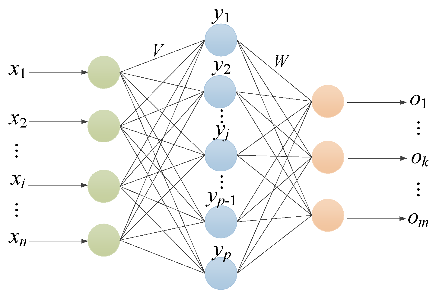
2.1. BPANN

Theoretically, it has been proven that for a three-layer BPANN, as long as there are enough neurons in the hidden layer, it can fit any complex nonlinear function, which shows that the BPANN has a strong fitting ability. The structure of the three-layer BPANN is shown in Figure 1. The formulas and charts related to neural networks involved in this section can be found in the literature [24].

In Figure 1, the input sample is X = (X₁, X₂, …, X_r, …, X_S)^T, X_r = (x₁, x₂, …, x_i, …, x_n)^T. The output of the hidden layer is Y = (Y₁, Y₂, …, Y_r, …, Y_S), and the output of the hidden layer corresponding to the sample X_r is Y_r = (y₁, y₂, …, y_j, …, y_p)^T. The output of the output layer is O = (O₁, O₂, …, O_r, …, O_S). The output of the output layer corresponding to the sample X_r is O_r = (o₁, o₂, …, o_k, …, o_m)^T. The expected output is D = (D₁, D₂, …, D_r, …, D_S), and the expected output corresponding to the sample X_r is D_r = (d₁, d₂, …, d_m)^T. The weight matrix between the input layer and the hidden layer is V = (V₁, V₂, …, V_j, …, V_p), and V_j is the weight vector corresponding to the j-th neuron in the hidden layer. The weight matrix between the hidden layer and the output layer is W = (W₁, W₂, …, W_k, …, W_m), and W_k is the weight vector corresponding to the k-th neuron in the output layer.

For the r-th training sample, X_r, the sum of errors of all neurons in the output layer of the BPANN is recorded as E_r. The calculation formula of E_r is

$$E_r=0.5{\displaystyle \sum _{k=1}^m{\left(d_k-o_k\right)}^2}$$

(1)

The average value of the sum of errors of all samples is recorded as E_av, and the calculation formula of E_av is

$$E_{av}=\frac{1}{S}{\displaystyle \sum _{r=1}^S{E}_r}$$

(2)

where S is the number of samples.

First, it is judged whether E_av meets the given error accuracy requirements. If it does, the training is stopped, and the optimal weight and threshold are output; otherwise, the weights and thresholds are adjusted until the given accuracy requirements are met.

To calculate the value of E_r, it is necessary to calculate the output of the output layer. Let the output of the output layer be O_r = (o₁, o₂, …, o_k, …, o_m)^T, and the net input of the output layer be net_k. For the output layer, there are

$$o_k=f(ne{t}_k) k=1,2,\dots ,m$$

(3)

$$ne{t}_k={\displaystyle \sum _{j=0}^p{w}_{jk}{y}_j} k=1,2,\dots ,m$$

(4)

Let the net input of the hidden layer be net_j; then, the calculation formulas of the net input net_j and output y_j of the hidden layer are

$$y_j=f(ne{t}_j) j=1,2,\dots ,p$$

(5)

$$ne{t}_j={\displaystyle \sum _{i=0}^n{v}_{ij}{x}_i} j=1,2,\dots ,p$$

(6)

In Equations (3) and (5), the activation functions are Sigmoid functions. The Sigmoid function is as follows

$$f(x)=\frac{1-e^{-x}}{1+e^{-x}}$$

(7)

The derivative of f(x) is

$$f\prime (x)=\frac{1}{2}[1-f{(x)}^2]$$

(8)

With the expansion of E_r in Equation (1) to the hidden layer, the calculation formula of E_r is

$$E_r=0.5{\displaystyle \sum _{k=1}^m{\left[d_k-f(ne{t}_k)\right]}^2}=0.5{{\displaystyle \sum _{k=1}^m\left[d_k-f\left({\displaystyle \sum _{j=0}^p{w}_{jk}{y}_j}\right)\right]}}^2$$

(9)

E_r in Equation (9) is expanded to the input layer, and there is

$$\begin{array}{c}{E}_r=0.5{\displaystyle \sum _{k=1}^m{\left\{d_k-f\left[{\displaystyle \sum _{j=0}^p{w}_{jk}f(ne{t}_j)}\right]\right\}}^2}=0.5{\displaystyle \sum _{k=1}^m{\left\{d_k-f\left[{\displaystyle \sum _{j=0}^p{w}_{jk}f({\displaystyle \sum _{i=0}^n{v}_{ij}{x}_i})}\right]\right\}}^2}\\ \end{array}$$

(10)

From Equations (2) and (10), there is

$$E_{av}=\frac{1}{S}{\displaystyle \sum _{r=1}^S{E}_r}=\frac{1}{2S}{\displaystyle \sum _{r=1}^S{\displaystyle \sum _{k=1}^m{\left\{d_{rk}-f\left[{\displaystyle \sum _{j=0}^p{w}_{jk}f({\displaystyle \sum _{i=0}^n{v}_{ij}{x}_{ri}})}\right]\right\}}^2}}$$

(11)

It can be seen from Equation (11) that the size of E_av can be changed by adjusting the weights. When E_av ≤ e (e is a sufficiently small positive number) or the preset learning times are reached, the training process is ended. Otherwise, the weights and thresholds of each layer are adjusted to gradually reduce E_av.

2.2. MOA

MOA is a swarm intelligence optimization algorithm based on the flight and reproduction behavior of mayflies. Suppose that an initial population X with size n is randomly generated, X = (X₁, X₂,…, X_i,…, X_n), X_i = (x_i1, x_i2,…, x_iD), and D is the dimension of the variable. X is divided into two groups: one is male mayflies, and the other is female mayflies. The velocity of each mayfly in the population is V, where V = (V₁, V₂,…, V_i,…, V_n),V_i = (v_i1, v_i2,…, v_iD). Let pbest_i be the historically optimal position of the i-th mayfly in the population, and gbest be the historically optimal position of all mayflies in the population. The formula of each part of the standard mayfly optimization algorithm involved in this section can be found in the literature [13].

2.2.1. Position and Velocity Updates of Male Mayflies

Male mayflies gather in groups a few meters above the water to perform courtship dances. They move according to their own and other individuals’ experiences, but not at a rapid rate. Let $x_t$I be the position of the i-th male mayfly at the t-th iteration, and $v_i^t$ be the velocity of the i-th male mayfly at the t-th iteration. The position update formula for male mayflies is as follows

$$x_i^{t+1}=x_i^t+v_i^{t+1}$$

(12)

The velocity update formula of male mayflies is

$$v_i^{t+1}=v_i^t+a_1{\mathrm{e}}^{-\beta r_p^2}\left(pbes{t}_i-x_i^t\right)+a_2{\mathrm{e}}^{-\beta r_g^2}\left( gbest-x_i^t\right)$$

(13)

where a₁ is the individual cognitive coefficient, and a₂ is the social contribution coefficient; usually, a₁ = 1, while a₂ = 1.5. β is the visibility coefficient controlling the visible range of a mayfly; usually, β = 2. r_p is the Euclidean distance between the i-th mayfly and pbest, while r_g is the Euclidean distance between the i-th mayfly and gbest.

The velocity update formula of the best male mayfly in the population is

$$v_i^{t+1}=v_i^t+d\times r i=1,2,\cdots ,n/2$$

(14)

where d is the dance coefficient—usually, d = 0.1—and r is a D-dimensional random vector evenly distributed between [−1,1].

2.2.2. Position and Velocity Updates of Female Mayflies

Each female mayfly has its own corresponding mate. Male and female mayflies are paired in order, that is, the best male mayfly mates with the best female mayfly, and the suboptimal male mayfly mates with the suboptimal female mayfly. When its spouse is better than itself, the female mayfly moves toward its spouse; otherwise, the female mayfly will randomly walk.

Let $y_i^t$ be the position of the i-th female mayfly at the t-th iteration. The position update formula of the female mayflies is

$$y_i^{t+1}=y_i^t+v_i^{t+1} i=0.5n+1,0.5n+2,\cdots ,n$$

(15)

The velocity update formula of the female mayflies is

$$v_i^{t+1}=\{\begin{array}{ll}{v}_i^t+a_2{\mathrm{e}}^{-\beta r_m^2}\left(x_i^t-y_i^t\right)\hfill & if \left(y_i\right)>f\left(x_i\right)\hfill \\ v_i^t+f_l\times r\hfill & otherwise \hfill \end{array}$$

(16)

where r_m is the Euclidean distance between a female mayfly and its spouse, f_l is the random walk coefficient—usually, f_l = 0.1—and r is a D-dimensional random vector evenly distributed between [−1,1].

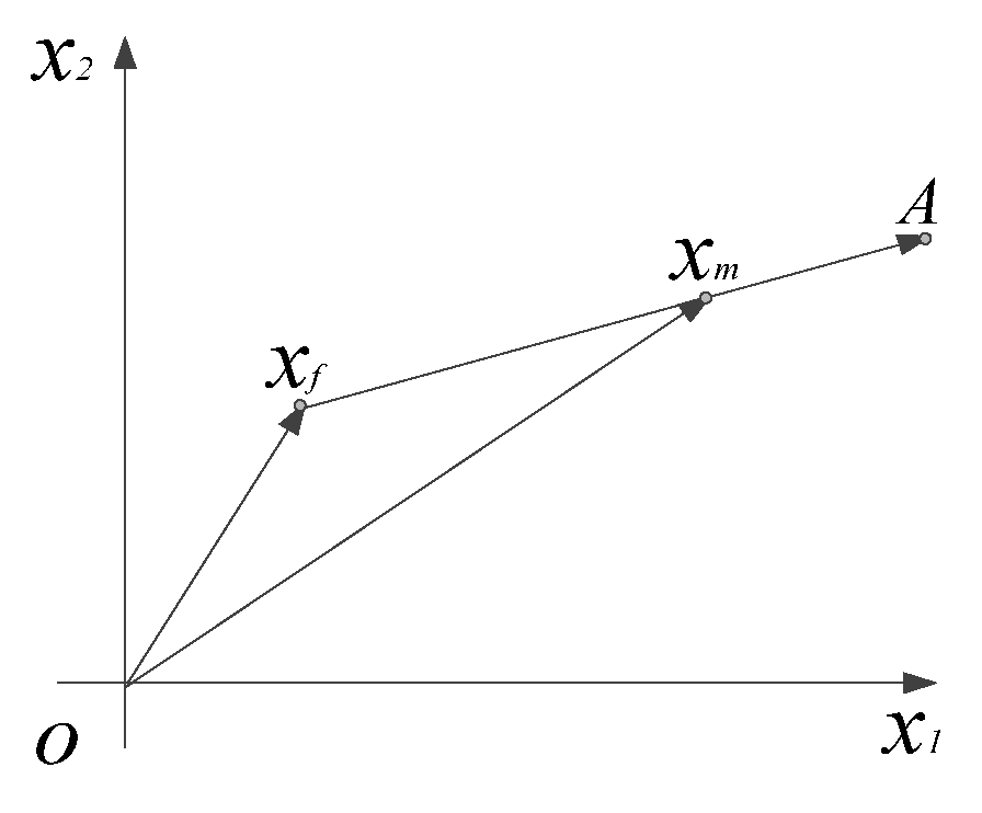
2.2.3. Mating of Mayflies

During the mating process, the optimal individual of the male mayflies mates with the optimal individual of the female mayflies, the suboptimal individual of male mayflies mates with the suboptimal individual of female mayflies, and so on. Supposing that the male mayfly involved in mating is x_m, and the female mayfly is x_f, the two offspring individuals obtained after mating are offspring1 and offspring2. The formulas for mating x_f and x_m to produce offspring are as follows:

$$\mathit{offspring}1=L*x_m+(1-L)*x_f$$

(17)

$$\mathit{offspring}2=L*x_f+(1-L)*x_m$$

(18)

In Equations (17) and (18), L is a random number uniformly distributed between [−1,1].

3. Improved Mayfly Optimization Algorithm with Adaptive Visibility Coefficient

3.1. Improved Velocity Update Formula

Because there is a coefficient $e^{-\beta r^2}$ in the velocity update formula of MOA in the existing literature, when the distance r between the mayflies is large, the value of $e^{-\beta r^2}$ approaches 0. If the value range of the variable is large, or the distance between the mayflies is large at the beginning iteration, the velocity update formula with the coefficient $e^{-\beta r^2}$ is almost ineffective. The trend of $e^{-\beta r^2}$ with r is shown in Figure 2.

It can be seen from Figure 2 that when the distance between mayflies is r ≥ 2, the value of $e^{-\beta r^2}$ approaches 0. At this time, except for the random walk mayflies, the velocity update formula of most mayflies in the population almost does not work, resulting in almost no update of the position of these mayflies, so potential mayflies cannot be generated. Therefore, when the distance between mayflies is r ≥ 2, the velocity update formula is not instructive, and MOA has a slow convergence speed and weak global search ability. In addition, when the problem is to be optimized with a large range of variable values, the distance between the mayflies is relatively far at the beginning of iteration, $e^{-\beta r^2}$ approaches 0, and the attraction term does not work. As the number of iterations increases, the distance between the mayflies gradually decreases. When r ≤ 2, the attraction term begins to work, and the heuristic of the velocity update formula gradually increases. The algorithm has a slow convergence speed in the early stage of iteration and a fast convergence speed in the later stage. To solve the above problems, an improved velocity update formula is proposed.

(a)

Improved velocity update formula of male mayflies:

$$v_i^{t+1}=v_i^t+a_1\beta /(1{+\mathrm{r}}_p)\left(pbes{t}_i-x_i^t\right)+a_2\beta /(1{+r}_g)\left( gbest-x_i^t\right)$$

(19)

where a₁ is the individual cognitive coefficient, and a₂ is the social contribution coefficient; usually, a₁ = 1, while a₂ = 1.5. r_p is the Euclidean distance between the i-th mayfly and pbest, while r_g is the Euclidean distance between the i-th mayfly and gbest. The best male mayfly in the population still updates its velocity according to Equation (14).

(b)

Improved velocity update formula of female mayflies:

$$v_i^{t+1}=\{\begin{array}{ll}{v}_i^t+a_2\beta /(1{+r}_m)\left(x_i^t-y_i^t\right)\hfill & if \left(y_i\right)>f\left(x_i\right)\hfill \\ v_i^t+f_l\times r\hfill & \mathit{otherwise} \hfill \end{array}$$

(20)

where r_m is the Euclidean distance between female mayflies and their spouses, and f_l is the random walk coefficient; usually, f_l = 0.1, and r is a D-dimensional random vector evenly distributed between [−1,1].

The improved velocity update formula solves the problem that the disturbance term caused by the distance fluctuation not working, and it avoids the situation of the algorithm stagnating and easily falling into a local optimum because the velocity and position of some mayflies are not updated in the search process. The heuristic and search ability of the improved algorithm are enhanced.

3.2. Adaptive Visibility Coefficient

In the existing MOA, the value of β is a constant. If the value of β is large, the exploration ability of the algorithm is strong. If the value of β is small, the algorithm’s development ability is strong. Therefore, when β is a constant, MOA cannot better balance the exploration and exploitation capabilities of the algorithm. Aiming at this problem, a calculation formula of adaptive change for β is given as follows

$$\beta =\left(1.8-\frac{runtime}{Maxtime}\right)(0.8+0.1*rand)$$

(21)

where Maxtime is the maximum running time of the algorithm set in advance, runtime is the time the algorithm has run so far, and rand is a random number between [0,1].

Because a₁ and a₂ are constants, the effect of the attraction term on velocity in Equations (19) and (20) depends on the values of β/(1 + r_p), β/(1 + r_g) and β/(1 + r_m). β/(1 + r_g) can be taken as an example to analyze the change trend of β/(1 + r_g) with the number of iterations. The C01 test function in CEC 2017 is selected, and the maximum running time of the algorithm is set to 20 s. Taking β/(1 + r_g) in the male mayflies update formula as an example, the value of β/(1 + r_g) of the 10th male mayfly in the population is recorded every 100 iterations. The trend of β/(1 + r_g) with the increase of the number of iterations is shown in Figure 3.

It can be noticed from Figure 3 that as the number of iterations increases, the overall trend of β/(1 + r_g) increases first and then decreases. The value of β/(1 + r_g) increases gradually at the beginning of iteration and decreases with oscillations later in iteration. Therefore, the exploration ability of a male mayfly is strong in the early stage of iteration, and the exploitation ability of male mayfly is strong in the later stage of iteration. In the whole iteration process, β/(1 + r_g) does not approach 0. In summary, the improved velocity update formula can better balance the exploration and exploitation capabilities of the algorithm and help to improve the performance of the algorithm.

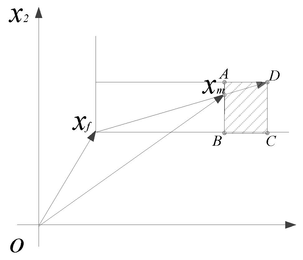
3.3. Improved Mayflies Mating Operator

The mating operator L in the existing MOA literature is a random number in a given range, and the two offspring mayflies produced by mating are located on the connection between the two parent mayflies. To illustrate the spatial position of the offspring mayflies produced by mating according to Equations (17) and (18), a two-dimensional space is taken as an example. It is assumed that the male mayfly involved in mating is X_m, the female mayfly is X_f, and L is a random number between [−1,1]. The spatial position of the offspring mayflies produced by mating is shown in Figure 4 and Figure 5.

In Figure 4, the spatial position of the mayflies produced by mating according to Equation (17) is on the line segment X_fA. Also, the spatial position of the offspring mayflies produced by mating according to Equation (18) is on the line segment AX_m. As the saying goes, ‘One who nears vermilion becomes red, and one who nears ink becomes black’, so the male mayflies among the two parental mayflies have a greater probability of being near the optimal solution. Because X_m is superior to X_f, the offspring of mating mayflies should be located near the male mayflies in the parent generation, which is more likely to produce potential offspring mayflies. However, the offspring mayflies produced by mating according to Equations (17) and (18) have only a small probability of being located near X_m, can only be located on the line X_fA or AX_m connecting X_f and X_m and cannot be located in other areas near X_m.

In order to overcome the problems of the mating operators in Equations (17) and (18), an improved mating operator is proposed, which causes the offspring mayflies produced by mating to be located near the male mayflies. The specific mating operators are as follows

offspring1 = L₁⊙X_m + (1−L₁)⊙X_f

(22)

offspring2 = L₂⊙X_f + (1−L₂)⊙X_m

(23)

where ⊙ denotes the multiplication of two vectors or the multiplication of elements at the same position in the matrix, L₁ is a D-dimensional random vector that is uniformly distributed between [0,0.5], and L₂ is a D-dimensional random vector that is uniformly distributed between [0.5,1].

The spatial positions of the offspring mayflies produced by mating according to Equations (22) and (23) are shown in Figure 6 and Figure 7.

The spatial positions of the offspring mayflies produced by mating according to Equations (22) and (23) are the shadowed parts in the figures. It can be seen from Figure 6 and Figure 7 that the probability that the offspring mayflies produced by mating according to Equations (22) and (23) are located near X_m is much higher than that produced by mating according to Equations (17) and (18). Therefore, compared with Equations (17) and (18), mating according to Equations (22) and (23) is more likely to produce more potential offspring individuals.

3.4. Time Complexity Analysis

The time complexity of the algorithm is an important indicator reflecting the advantages and disadvantages of the algorithm, so this section analyzes the time complexity of the proposed AVC-IMOA. The following components are primarily responsible for increasing the time complexity of AVC-IMOA: the generation of the initial population, the speed and position updating of male mayflies, the speed and position updating of female mayflies and the mating operation of male and female mayflies. These four operations are represented by ①, ②, ③ and ④, respectively. Suppose the population size is n, the number of male mayflies is n/2, the number of female mayflies is n/2, and the dimension of the variable is D. The time complexity analysis is summarized in

Table 1. The time complexity of AVC-IMOA.

Names of Various Operators	①	②	③	④	AVC-IMOA
Time complexity	O(n)	O(n/2)	O(n/2)	O(n/2)	O(n) + O(n/2) + O(n/2) + O(n/2) = O(n)

.

3.5. Flow Chart of AVC-IMOA

Taking the objective function minimization as an example, the flow chart of AVC-IMOA is shown in Figure 8.

3.6. Pseudocode of AVC-IMOA

A maximum running time for the algorithm, denoted as Maxtime, is set. When the algorithm runs to a set maximum, it then stops running and outputs the final result. The pseudocode of the improved mayfly optimization algorithm with an adaptive visibility coefficient is shown in Algorithm 1.

Algorithm 1: Improved mayfly optimization algorithm with adaptive visibility coefficient (AVC-IMOA)

Begin

Randomly generate an initial population with size n and calculate the fitness values of all individuals.

The global optimal position gbest of all mayflies and the optimal position pbest of male mayflies were recorded. Runtime = 0

Whileruntime ≤ Maxtime do

Update the position and velocity of male mayflies according to Equations (12), (14), (19) and (21).

Update the position and velocity of female mayflies according to Equations (15), (20) and (21).

Male and female mayflies mate according to Equations (22) and (23) to produce offspring.

Process the individuals beyond the search scope.

Recalculate the fitness values of all mayflies and retain n better individuals.

Update gbest and pbest.

End while

Output the optimal solution and the optimal value.

End

4. Numerical Experiments and Analysis

The CEC 2017 test function set is currently the internationally used test function set to measure algorithm performance. All constrained optimization problems in the test function set are minimization problems. To test the performance of the proposed AVC-IMOA, the CEC 2017 test function set [25] is selected as a source of test functions.

4.1. Algorithm Performance Evaluation Indicator

In order to compare the performance of AVC-IMOA and various comparison algorithms, the mean value (Mean), standard deviation (Std) and Friedman rank ranking of algorithms are used as performance evaluation indicators [26].

• Mean

The mean value is defined as the average of the optimal value of the test function obtained by the algorithm in R independent runs, and is recorded as Mean. The calculation formula of Mean is

$$Mean=\frac{{\displaystyle {\sum }_{i=1}^R{f}_i}}{R}$$

(24)

where R is the total number of independent runs of the algorithm, and f_i is the optimal value of the test function obtained when the algorithm runs independently for the i-th time.

2.

Std

The standard deviation can reflect the dispersion degree between the optimal value obtained by R operations of an algorithm and the average value of R optimal values. The standard deviation is recorded as Std. A large Std represents a large difference between most of the optimal values and their averages; a smaller Std means that the optimal value is closer to the average. Therefore, the smaller the Std, the better the robustness of the algorithm. The calculation formula for Std is

$$Std=\sqrt{\frac{{\displaystyle {\sum }_{i=1}^R{(f_i-Mean)}^2}}{R}}$$

(25)

3.

w/t/l

To better compare the performance of AVC-IMOA with the various algorithms involved in the comparison, the comparison result of the Mean of AVC-IMOA with another algorithm (denoted as, Alg1) involved in the comparison is denoted as w/t/l. For a test function, if the performance of the AVC-IMOA algorithm is better than Alg1, the value of w is denoted as 1. If the performance of the AVC-IMOA algorithm is the same as that of Alg1, the value of t is denoted as 1. If Alg1 performs better than AVC-IMOA, the value of l is recorded as 1. For all test functions, adding the value of w = 1 in Alg1 and AVC-IMOA yields the value of w. Similarly, the values of t and l can be calculated.

4.

Friedman rank ranking

Friedman rank ranking is a nonparametric statistical method which can rank the performance of algorithms involved in comparison [26]. When the number of algorithms participating in the comparison is m and the number of selected test functions is k, the Friedman ranking of the algorithm can be calculated according to the following steps.

(1)

Each algorithm runs R times independently on each test function and retains the optimal value for each run.

(2)

According to Equation (24), the average value of the optimal value obtained from R runs is calculated.

$$Mea{n}_i^j=\frac{{\displaystyle \sum _{l=1}^R{f}_i^j(l)}}{R},i=1,2,\dots m; j=1,2,\dots k$$

(26)

where m is the number of algorithms involved in the comparison, k is the number of test functions, R is the number of independent runs, and meanf_i^j is the average value of the optimal value obtained by the i-th algorithm independently running R times on the j-th test function.

(3)

For each test function, m algorithms are sorted in accordance with the meanf_i^j from small to large and given the rank_i^j(i = 1, 2,…, m; j = 1, 2,…, k) of each algorithm. Sometimes there will be cases where the algorithms involved in the comparison obtain the same meanf_i^j; in this case, the average value of the ranking position is taken as the rank ranking.

(4)

According to Equation (27), the Averank_i of each algorithm is calculated.

$$Averan{k}_i=\frac{1}{m}{\displaystyle \sum _{j=1}^{k}ran{k}_i^j} , i=1,2,\dots m$$

(27)

(5)

After sorting by the Averank_i of each algorithm from small to large, the sorting result is the final ranking of the various algorithms.

4.2. Parameter Setting

To verify the performance of AVC-IMOA, four MOA algorithms and two meta-heuristic algorithms are selected for comparison. These are the algorithms involved in the comparison: standard MOA (MOA) [13], MOA with velocity processing and gravity coefficient (VGMOA) [13], MOA with improved velocity update formula (IMOA) [18], MOA with opposition-based learning rules (OBL_MO) [19], sparrow search algorithm (SSA) and opposition-based learning particle swarm optimization by group decision-making (OBLPSOGD) [27]. The parameters of the algorithms involved in the comparison are all the values found in the original literature, and the specific parameter values are shown in

Table 2. Algorithms and parameter settings involved in the comparison.

Algorithm	Year	Parameters
MOA	2020	α1 = 1, α2 = 1.5, β = 2, d = 0.1, fl = 0.1
VGMOA	2020	α1 = 1, α2 = 1.5, β = 2, d = 0.1, fl = 0.1, gmax = 0.9, gmin = 0.5
IMOA	2020	α1 = 1, α2 = 1.5, β = 2, d = 0.1, fl = 0.1
OBL_MO	2020	α1 = 1, α2 = 1.5, β = 2, d = 0.1, fl = 0.1
OBLPSOGD	2018	wmin = 0.4, wmax = 0.9, P0 = 0.3, α = 3.2, k = 15, σ =0.3
SSA	2020	PD = 0.2NP, SD = 0.1NP, ST = 0.8
AVC-IMOA	2022	α1 = 1, α2 = 1.5, d = 0.1. fl = 0.1

.

4.3. Test Results and Analysis

4.3.1. Test Results

To ensure that the experimental results are fair and reasonable, all test experiments are completed on the same computer. All experiments in this paper are carried out in the same operating environment, that is, under the Windows 10 system, using an AMD Ryzen 9 3900 12-core Processor CPU @ 3.09 GHz desktop computer. The software and version used are: MATLAB R2019b. Let the population size of the seven algorithms be n = 30, the dimension of the variable be D = 30 and the maximum running time be Maxtime = 20 s. When the algorithm reaches the maximum running time, stop the iteration and output the optimal solution and optimal value. Each test function runs 25 times independently, and the Mean and Std of the optimal values of each test function obtained by each algorithm are recorded. The results of each algorithm on the CEC 2017 test function set are shown in

Table 3. Calculation results of each algorithm.

Problem	Statistical Indicators	Algorithm
		MOA	VGMOA	IMOA	OBL_MO	SSA	OBLPSOGD	AVC-IMOA
C01	Mean	1.36 × 10-2	8.05 × 10-3	1.69 × 10-1	2.89 × 10-2	1.44 × 105	7.88 × 102	2.22 × 10-13
	Std	5.09 × 10-3	3.21 × 10-3	4.16 × 10-2	1.55 × 10-2	4.01 × 104	3.37 × 102	7.81 × 10-13
C02	Mean	2.53 × 10-2	1.16 × 10-2	2.12 × 10-1	2.80 × 10-2	5.32 × 104	1.61 × 103	3.99 × 10-10
	Std	8.39 × 10-3	4.15 × 10-3	3.28 × 10-2	1.18 × 10-2	1.51 × 104	7.26 × 102	1.54 × 10-9
C03	Mean	2.94 × 105	1.02 × 106	3.81 × 106	1.80 × 106	9.21 × 107	6.45 × 104	6.53 × 105
	Std	6.49 × 105	1.48 × 106	3.20 × 106	3.13 × 106	3.32 × 107	2.94 × 104	1.07 × 106
C04	Mean	8.79 × 102	9.16 × 102	9.01 × 102	8.81 × 102	6.17 × 102	5.67 × 102	6.57 × 102
	Std	6.95 × 101	4.15 × 101	5.67 × 101	6.55 × 101	2.71 × 101	6.27 × 101	1.92 × 101
C05	Mean	3.75 × 101	4.18 × 101	5.75 × 101	3.87 × 101	6.74 × 105	4.98 × 102	1.97 × 101
	Std	2.68 × 101	2.75 × 101	6.17 × 101	2.67 × 101	6.76 × 104	3.43 × 102	6.43 × 100
C06	Mean	1.00 × 108	5.30 × 107	6.32 × 108	6.70 × 107	1.19 × 1010	1.25 × 109	2.98 × 107
	Std	1.43 × 108	1.07 × 108	1.51 × 108	1.44 × 108	4.76 × 109	4.43 × 109	1.03 × 108
C07	Mean	8.46 × 102	1.25 × 104	1.09 × 1012	3.74 × 102	7.67 × 1013	−7.28 × 101	−3.06 × 102
	Std	5.25 × 103	6.33 × 104	1.70 × 1011	2.20 × 103	1.64 × 1013	1.41 × 102	1.47 × 102
C08	Mean	1.61 × 103	1.86 × 103	1.04 × 106	9.89 × 103	1.63 × 1017	1.17 × 1013	7.19 × 10-4
	Std	9.05 × 102	1.41 × 103	4.62 × 105	6.80 × 103	5.98 × 1016	8.10 × 1012	3.31 × 104
C09	Mean	7.25 × 100	6.22 × 100	4.02 × 106	6.79 × 100	8.31 × 1013	8.91 × 1011	2.18 × 100
	Std	2.40 × 100	1.88 × 100	1.24 × 107	2.31 × 100	4.30 × 1013	2.2 × 1012	2.97 × 100
C10	Mean	3.71 × 101	3.16 × 101	1.19 × 106	2.18 × 102	3.12 × 1018	2.23 × 1013	2.76 × 10-4
	Std	5.08 × 101	2.97 × 101	5.67 × 105	2.48 × 102	9.28 × 1017	2.07 × 1013	8.29 × 105
C11	Mean	2.65 × 1012	4.61 × 1011	4.86 × 1013	3.93 × 1012	2.14 × 1017	8.92 × 1016	5.87 × 1010
	Std	4.40 × 1012	7.24 × 1011	6.45 × 1013	5.20 × 1012	8.61 × 1016	9.96 × 1016	1.01 × 1011
C12	Mean	9.68 × 101	8.05 × 101	1.29 × 102	1.09 × 102	2.59 × 1017	1.40 × 1012	1.31 × 101
	Std	3.36 × 101	2.83 × 101	2.85 × 101	3.88 × 101	4.99 × 1016	1.80 × 1012	9.76 × 100
C13	Mean	6.90 × 1014	1.78 × 1015	7.53 × 1015	1.80 × 1015	2.86 × 1017	1.57 × 1013	5.91 × 1014
	Std	3.77 × 1014	8.85 × 1014	2.66 × 1015	7.15 × 1014	3.93 × 1016	1.22 × 1013	2.45 × 1014
C14	Mean	1.94 × 100	1.97 × 100	2.06 × 100	1.97 × 100	5.25 × 1017	2.77 × 1012	1.41 × 100
	Std	7.63 × 10-2	7.50 × 10-2	8.48 × 10-2	9.82 × 10-2	5.42 × 1016	5.22 × 1012	2.02 × 102
C15	Mean	2.31 × 101	2.45 × 101	2.37 × 101	2.27 × 101	2.32 × 1017	1.49 × 101	2.57 × 101
	Std	2.57 × 100	3.07 × 100	3.76 × 100	3.86 × 100	3.75 × 1016	1.60 × 100	5.37 × 100
C16	Mean	2.41 × 102	2.39 × 102	2.42 × 102	2.37 × 102	2.42 × 1017	1.34 × 102	1.32 × 102
	Std	1.01 × 101	9.88 × 100	1.27 × 101	1.15 × 101	3.50 × 1016	7.55 × 100	1.46 × 1016
C17	Mean	9.61 × 1010	9.61 × 1010	9.61 × 1010	9.61 × 1010	2.86 × 1017	1.44 × 1012	9.61 × 1010
	Std	7.62 × 10-3	3.93 × 10-3	9.95 × 10-3	5.34 × 10-3	3.44 × 1016	2.82 × 1012	4.44 × 102
C18	Mean	9.95 × 1014	4.78 × 1014	1.38 × 1015	6.52 × 1014	2.13 × 1028	3.80 × 1019	5.97 × 1010
	Std	1.65 × 1015	8.14 × 1014	2.57 × 1015	9.78 × 1014	4.43 × 1027	4.38 × 1019	1.68 × 1011
C19	Mean	1.85 × 1017	1.85 × 1017	1.85 × 1017	1.85 × 1017	1.85 × 1017	1.84 × 1017	1.83 × 1017
	Std	9.16 × 1013	7.14 × 1013	8.55 × 1013	7.91 × 1013	4.15 × 1013	1.84 × 1014	4.87 × 105
C20	Mean	2.89 × 100	3.10 × 100	7.61 × 100	2.76 × 100	8.27 × 100	8.26 × 100	2.50 × 100
	Std	5.11 × 10-1	6.82 × 10-1	2.79 × 10-1	4.44 × 10-1	3.51 × 10-1	4.10 × 10-1	4.49 × 10-1
C21	Mean	1.21 × 102	8.53 × 101	1.39 × 102	1.05 × 102	1.10 × 1017	6.58 × 1012	1.10 × 101
	Std	4.03 × 101	3.55 × 101	2.05 × 101	3.26 × 101	2.11 × 1016	6.22 × 1012	1.03 × 101
C22	Mean	7.30 × 1014	1.77 × 1015	5.77 × 1015	1.89 × 1015	1.17 × 1017	4.64 × 1013	8.46 × 1014
	Std	4.40 × 1014	9.42 × 1014	2.04 × 1015	9.23 × 1014	1.72 × 1016	3.74 × 1013	5.17 × 1014
C23	Mean	1.97 × 100	1.99 × 100	2.04 × 100	1.97 × 100	2.00 × 1017	1.92 × 1013	1.43 × 100
	Std	6.09 × 10-2	8.28 × 10-2	9.63 × 10-2	7.98 × 10-2	3.46 × 1016	2.80 × 1013	3.23 × 10-2
C24	Mean	2.32 × 101	2.17 × 101	2.37 × 101	2.36 × 101	9.18 × 1016	1.59 × 101	2.35 × 101
	Std	4.43 × 100	2.51 × 100	2.99 × 100	4.08 × 100	1.17 × 1016	1.45 × 100	3.80 × 100
C25	Mean	2.42 × 102	2.38 × 102	2.43 × 102	2.40 × 102	8.46 × 1016	1.39 × 102	2.42 × 102
	Std	1.09 × 101	9.58 × 100	9.05 × 100	1.14 × 101	1.72 × 1016	1.01 × 101	1.30 × 101
C26	Mean	9.61 × 1010	9.61 × 1010	9.61 × 1010	9.61 × 1010	1.17 × 1017	5.00 × 1012	9.61 × 1010
	Std	3.42 × 10-3	3.14 × 10-3	3.05 × 10-3	6.69 × 10-3	1.71 × 1016	7.47 × 1012	4.74 × 10-2
C27	Mean	2.01 × 1013	7.94 × 1013	6.84 × 1014	2.35 × 1014	5.86 × 1027	3.99 × 1019	8.14 × 1012
	Std	2.33 × 1013	2.74 × 1014	1.05 × 1015	7.13 × 1014	1.07 × 1027	5.09 × 1019	1.77 × 1013
C28	Mean	1.85 × 1017	1.85 × 1017	1.85 × 1017	1.85 × 1017	1.85 × 1017	1.84 × 1017	1.85 × 1017
	Std	1.10 × 1014	1.12 × 1014	9.35 × 1013	8.29 × 1013	7.60 × 1013	2.42 × 1014	1.42 × 1014
Mean: w/t/l		26/2/0	25/2/1	26/2/0	26/2/0	28/0/0	21/0/7	-

, and the best results for each test function have been bolded. The Friedman mean rank and final rank ranking results of each algorithm are shown in Figure 9.

4.3.2. Result Analysis

(1)

Result analysis of test function

It can be seen from Table 3 that the quality of VGMOA is the best when using the above seven algorithms to solve the C17 and C25 test functions. When solving the C26 test function, the solution quality of IMOA is the best. When solving the seven test functions C03, C04, C13, C15, C22, C24 and C28, the solution quality of OBLPSOGD is the best. When solving the other 19 test functions, AVC-IMOA has the best solution quality. According to the value of w/t/l in Table 3, the performance of AVC-IMOA is better than the other six algorithms.

As can be observed from Figure 9, AVC-IMOA ranks first among all algorithms when the dimension of the variable is D = 30, which indicates that the performance of AVC-IMOA is better than the other six algorithms involved in the comparison.

In addition, in order to verify whether there are significant differences in the performance of the above seven algorithms, the Friedman test method is selected. The Friedman test was first proposed by Friedman in 1945 as a nonparametric test method to determine whether there are significant differences between algorithms [28]. The Friedman test results of the seven algorithms are shown in

Table 4. Friedman test results for each algorithm.

Dimension	Significance Level	Number of Algorithms	χ2	χ2 α[k−1]	p-Value	Null Hypothesis	Alternative Hypothesis
D = 30	α = 0.05	7	91.62	12.50	1.39345×10−17	Reject	Accept

.

Table 4 shows that when the significance level is α = 0.05, the critical value is χ2 α[k−1] = 12.50, while the test value is χ² = 91.62. Therefore, χ² > ${\chi }_{\alpha [k-1]}^2$, which shows that there are significant differences in the performances of the above seven algorithms.

To sum up, from the running results of each algorithm on the CEC 2017 test function set, the performance of AVC-IMOA is better than the other six algorithms, and the performance of each algorithm is significantly different, thus verifying the effectiveness of AVC-IMOA.

(2)

Convergence curve analysis

To verify the convergence of AVC-IMOA, two unimodal test functions, C01 and C02, and two multimodal test functions, C10 and C18, are selected to draw the convergence curves of AVC-IMOA and the other algorithms. The convergence curves are shown in Figure 10, where the x-axis represents the running time of the algorithms and the y-axis represents the fitness function value.

It can be seen from Figure 10 that when calculating the 30-dimensional test function, for the test function C01, AVC-IMOA and SSA have a fast convergence speed early in iteration, which indicates that AVC-IMOA and SSA have strong global search ability. In addition, the solution accuracy of AVC-IMOA is higher than those of the six comparison algorithms, which indicates that AVC-IMOA can not only jump out of a local optimum, but also has strong local search ability. For the test function C02, AVC-IMOA has a faster convergence speed and higher solution accuracy than the other six comparison algorithms, which shows that AVC-IMOA has global search ability and local search ability. For the C10 test function, the convergence speed of AVC-IMOA is faster in the early stage of iteration. In the middle stage of iteration, AVC-IMOA has the same effect as MOA, VGMOA and OBL_MO, but AVC-IMOA has higher accuracy in the later stage of iteration. Other algorithms fall into a local optimum. It can be seen that the global search ability of AVC-IMOA is better those that of the six comparison algorithms. For the test function C18, AVC-IMOA converges faster than the other six comparison algorithms throughout the iteration process, indicating that AVC-IMOA has strong global search ability.

4.4. AVC-IMOA to Optimize BPANN

Because the error function of a BPANN is a nonlinear multi-extremum optimization problem, it is easy to fall into a local optimum when the weights and thresholds of the BPANN are adjusted by the gradient method. When the number of neurons in each layer of a BPANN is large, the number of weights and thresholds is large, that is, there are many variables to be optimized, and it is difficult for the gradient method to obtain satisfactory results in a short time. In recent years, intelligent optimization algorithms have been used to optimize the weights and thresholds of BPANNs, and good results have been achieved. However, when there are many weights and thresholds to be optimized, there are problems such as low optimization accuracy and a poor solution effect. Therefore, an improved algorithm with an adaptive visibility coefficient is proposed to optimize the weights and thresholds of the BPANN.

Because the error function of a BPANN is a function with weights and thresholds as variables, the error function E_av in Equation (11) can be used as the objective function, and the weights and thresholds in Equation (11) can be used as variables. AVC-IMOA is used to optimize the objective function, and the optimal weights and thresholds are given when the iteration termination conditions are satisfied.

5. Prediction of Pork Supply

5.1. Sample Data

The data for pork supply in Heilongjiang Province can be obtained from the China Animal Husbandry and Veterinary Yearbook. The data for pork supply in Heilongjiang Province are shown in

Table 5. Pork supply in Heilongjiang province from 2000 to 2020 (unit: 10,000 tons).

Year	Supply	Year	Supply	Year	Supply
2000	89.0365	2007	101.68	2014	133.4
2001	87.1	2008	92.11	2015	142.6
2002	73.1	2009	96.6	2016	138.4
2003	82.4	2010	108.2	2017	138.2
2004	85.57	2011	114.48	2018	159.3
2005	93.87	2012	116.9	2019	149.9
2006	100.44	2013	128.4	2020	135.2

.

When using a BPANN to predict pork supply, sample data need to be normalized. The normalization processing formula is

$$X_{\mathit{new}}=a+(b-a)\left(\frac{X-X_{\min }}{X_{\max }-X_{\min }}\right)$$

(28)

where X is the sample data, X_new is the normalized sample data, X_max and X_min are the maximum and minimum values in the sample data, respectively, and a and b are the lower and upper limits of the data processing interval, respectively; usually, a = −0.8, b = 0.8.

The structure of the BPANN is 5-8-1, that is, the numbers of neurons in the input layer, hidden layer and output layer are 5, 8 and 1, respectively. The first training sample takes the data from 2000 to 2004 as input data, and the data from 2005 as the expected output; the second sample takes the data from 2001 to 2005 as input data and the data from 2006 as the expected output. By analogy, a total of 16 groups of sample data were obtained.

5.2. Prediction of Pork Supply

We take a sigmoid function as the activation function of the BPANN. Firstly, the weights and thresholds of the BPANN are initialized, that is, the initial weights and thresholds are randomly generated in the range of [−1,1], and the initial weights and thresholds are used as the initial population of AVC-IMOA. Secondly, taking the error function E_av as the objective function and the weights and thresholds as the variables to be optimized, the objective function is optimized by AVC-IMOA, and the optimal weights and thresholds of the BPANN are given. Finally, the trained BPANN is used to predict the pork supply in Heilongjiang Province from 2005 to 2022. The optimal weights and thresholds of the BPANN are shown in

Table 6. Optimal weights and thresholds of BPANN.

Vi,j	V1,1 = 2.1204	V2,1 = 0.2963	V3,1 = −2.1252		V4,1 = −1.8276		V5,1 = −1.6392
	V1,2 = −3.4353	V2,2 = −1.4154	V3,2 = −3.8704		V4,2 = −2.5717		V5,2 = 2.9983
	V1,3 = −2.8525	V2,3 = −0.5859	V3,3 = −0.8830		V4,3 = −2.2500		V5,3 = 2.5122
	V1,4 = 2.0599	V2,4 = −1.8145	V3,4 = −2.4980		V4,4 = 2.2324		V5,4 = −11.4764
	V1,5 = 0.7585	V2,5 = 2.8209	V3,5 = −9.8287		V4,5 = 3.2329		V5,5 = −3.2925
	V1,6 = −0.5469	V2,6 = 0.5614	V3,6 = −0.8615		V4,6 = 0.8089		V5,6 = 0.3829
	V1,7 = 1.4614	V2,7 = −0.3741	V3,7 = −3.5242		V4,7 = 2.1073		V5,7 = −0.8814
	V1,8 = −1.6766	V2,8 = 1.1384	V3,8 = −1.0364		V4,8 = −2.4203		V5,8 = 4.0111
T0	T0,1 = −1.7852	T0,2 = 5.8729	T0,3 = 0.2750	T0,4 = 2.4645	T0,5 = 1.7107	T0,6 = 0.1905	T0,7 = 0.6535	T0,8 = 0.4202
Wi,j	W1,1 = 3.3681	W2,1 = 1.7397	W3,1=−2.2738	W4,1 = −1.9837	W5,1 = 0.5642	W6,1=−3.6471	W7,1=−1.8537	W8,1 = 0.4153
T1	T1 = 1.6062

.

In Table 6, V is the weight matrix from the input layer to the hidden layer, W is the weight matrix from the hidden layer to the output layer, T₀ is the threshold of the hidden layer, and T₁ is the threshold of the output layer.

To verify the superiority of AVC-IMOA for optimizing the weights and thresholds of the BPANN, a BPANN based on the gradient descent method, a BPANN based on a mixed-strategy whale optimization algorithm (MSWOA_BP) [29], a BPANN based on the standard artificial bee colony algorithm (ABC_BP) [30] and a BPANN based on an improved sparrow search algorithm (FASSA_BP) [31] are selected as comparison algorithms. In addition, in order to fairly compare the performance and the accuracy of prediction of the different models, the structure of the BPANN is 5-8-1, the population size of the four intelligent optimization algorithms is 40, the sigmoid function is used as the transfer function, and the maximum running time of the five algorithms is 60 s. The prediction results and prediction accuracy are shown in

Table 7. Prediction accuracy and prediction results.

Year	Pork Supply Volume	BP (Gradient Descent)			MSWOA_BP			ABC_BP			FASSA_BP			AVC-IMOA_BP
		Predicted Value	Relative Error	Average Relative Error	Predicted Value	Relative Error	Average Relative Error	Predicted Value	Relative Error	Average Relative Error	Predicted Value	Relative Error	Average Relative Error	Predicted Value	Relative Error	Average Relative Error
2005	93.87	94.494	0.66470%	1.68000%	95.563	1.80358%	3.08207%	95.139	1.35233%	0.94325%	93.443	0.45456%	2.62584%	93.87000	0.000001%	0.000001%
2006	100.44	98.744	1.68853%		96.910	3.51436%		99.553	0.88350%		97.647	2.78110%		100.44000	0.000000%
2007	101.68	99.615	2.03126%		99.707	1.94045%		98.698	2.93291%		94.676	6.88786%		101.68000	0.000000%
2008	92.11	100.342	8.93669%		100.683	9.30729%		96.293	4.54162%		98.192	6.60249%		92.11000	0.000001%
2009	96.6	95.395	1.24786%		100.211	3.73802%		95.592	1.04387%		95.655	0.97802%		96.60000	0.000002%
2010	108.2	108.451	0.23230%		107.849	0.32455%		107.770	0.39724%		109.922	1.59178%		108.20000	0.000001%
2011	114.48	113.870	0.53328%		114.490	0.00870%		115.334	0.74561%		114.705	0.19661%		114.48000	0.000000%
2012	116.9	117.822	0.78886%		118.366	1.25445%		116.682	0.18688%		118.936	1.74168%		116.90000	0.000000%
2013	128.4	122.345	4.71590%		124.828	2.78191%		128.478	0.06087%		124.856	2.76015%		128.40000	0.000002%
2014	133.4	134.844	1.08244%		140.365	5.22096%		133.921	0.39041%		139.325	4.44143%		133.40000	0.000000%
2015	142.6	140.935	1.16729%		138.748	2.70093%		141.679	0.64612%		135.837	4.74294%		142.60000	0.000001%
2016	138.4	141.139	1.97878%		142.598	3.03344%		138.841	0.31868%		142.426	2.90931%		138.40000	0.000000%
2017	138.2	138.564	0.26325%		142.911	3.40883%		138.966	0.55450%		139.717	1.09803%		138.20000	0.000001%
2018	159.3	159.562	0.16418%		147.836	7.19677%		158.137	0.73001%		154.342	3.11262%		159.30000	0.000002%
2019	149.9	149.317	0.38882%		148.734	0.77765%		149.890	0.00634%		149.182	0.47915%		149.90000	0.000000%
2020	135.2	134.840	0.26604%		138.311	2.30117%		134.793	0.30111%		136.871	1.23579%		135.20000	0.000000%
2021		175.821			141.856			159.113			150.274			159.92
2022		153.896			148.885			153.209			154.735			161.26

. The fitting accuracy of the five models and the predicted value of pork supply are shown in Figure 11.

According to the data in Table 7, the average relative error of the BPANN is 1.68000%, while the average relative error of MSWOA_BP is 3.08207%; for ABC_BP, it is 0.94325%; for FASSA_BP, it is 2.62584%; and for AVC-IMOA_BP, it is 0.000001%. Therefore, the prediction accuracy of AVC-IMOA_BP is significantly higher than those of the BPANN, MSWOA_BP, ABC_BP and FASSA_BP.

As can be seen from Table 7 and Figure 11, the supply of pork in Heilongjiang Province of China was as high as 1.593 million tons in 2018, and the supply of pork decreased continuously in the following two years, reaching only 1.352 million tons in 2020. This is because the first outbreak of African swine fever in China occurred in August 2018. Since then, there have been sudden outbreaks of African swine fever throughout the country. A total of 800,000 live pigs were culled in 2018, and 390,000 live pigs were culled in 2019, resulting in a decrease in pork supply, higher pork prices, increased enthusiasm of farmers to raise pigs and an increase in the number of new, small sows and breeding sows. In addition, the African swine fever epidemic in China will be effectively controlled in 2020, and the pork supply in Heilongjiang Province will show a steady upward trend in 2021 and 2022. The pork supply numbers in Heilongjiang Province in 2021 and 2022 will be 1.5992 million tons and 1.6126 million tons, respectively.

6. Conclusions

When using the gradient method and existing intelligent optimization algorithms to optimize a BPANN, there are some shortcomings such as slow optimization speed and low precision. An improved MOA is proposed to optimize the weights and thresholds of a BPANN, and then the trained BPANN is used to predict the pork supply in Heilongjiang Province.

To improve the global optimization ability and solution accuracy of MOA, an improved mayfly optimization algorithm with an adaptive visibility coefficient was proposed. Firstly, focusing on the problem of the velocity update formula of some mayflies in the population not working when the distance between mayflies is large in the existing algorithm, an improved velocity update formula is proposed. The improved velocity update formula does not have the limitation that the velocity and position of an individual cannot be updated due to the large distance between individuals in the iterative process. Secondly, a method of adaptively adjusting the visibility coefficient is given, which makes the update method of the position and velocity of the algorithm have strong global search ability in the early stage of iteration and strong local search ability in the later stage of iteration; thus, the global search ability and local search ability of the algorithm are better balanced. Finally, in order to improve the probability of generating better potential solutions in the mating process of mayflies, an improved mating operator is given. The improved mating operator improves the solution quality and convergence speed of the algorithm.

AVC-IMOA is used to optimize the weights and thresholds of the BPANN with a network structure of 5-8-1. The BPANN determined by the obtained optimal weights and thresholds was adopted to predict the pork supply in Heilongjiang Province. In order to verify the performance of AVC-IMOA, AVC-IMOA_BP, a BPANN based on the gradient descent method, MSWOA_BP, ABC_BP and FASSA_BP were used to predict the pork supply in Heilongjiang Province. The prediction results show that the prediction accuracy of AVC-IMOA_BP is obviously better than those of other prediction models, which verifies the effectiveness of the proposed prediction method. In addition, it can be seen from the results that the pork supply in Heilongjiang Province will show a steady growth trend in 2021 and 2022, which can provide a reference for pig producers and governments at all levels to make decisions. Accurately predicting the pork supply lays the foundation for further study of pork price fluctuation and pork supply and demand balance.

In the future, there will be many fields worthy of our research and exploration. In addition to the speed update formula proposed in this paper, the performance of the algorithm will be further improved by starting with the position update formula, mutation method and hybrid algorithm. In addition, AVC-IMOA_BP can also be used to solve similar forecasting problems in production and life, not only for forecasting the supply of agricultural products.

References

1. Shen, Z.; Zhang, Y.; Lu, J.; Xu, J.; Xiao, G. A novel time series forecasting model with deep learning. Neurocomputing 2019, 396, 302–313. [Google Scholar] [CrossRef]
2. Kadiyala, A.; Kumar, A. Vector-time-series-based back propagation neural network modeling of air quality inside a public transportation bus using available software. Environ. Prog. Sustain. Energy 2015, 35, 7–13. [Google Scholar] [CrossRef]
3. Che, Z.-G.; Chiang, T.-A.; Che, Z. Feed-forward neural networks training: A comparison between genetic algorithm and back-propagation learning algorithm. Int. J. Innov. Comput. Inf. Control 2011, 7, 5839–5850. [Google Scholar]
4. Jie, Z.; Qiurui, M. Establishing a Genetic Algorithm-Back Propagation model to predict the pressure of girdles and to determine the model function. Text. Res. J. 2020, 90, 2564–2578. [Google Scholar] [CrossRef]
5. Cheng, P.; Chen, D.; Wang, J. Clustering of the body shape of the adult male by using principal component analysis and genetic algorithm–BP neural network. Soft Comput. 2020, 24, 13219–13237. [Google Scholar] [CrossRef]
6. Guo, K.; Cheng, X.; Shi, J. Accuracy Improvement of Short-Term Photovoltaic Power Forecasting Based on PCA and PSO-BP. In Proceedings of the 2021 3rd Asia Energy and Electrical Engineering Symposium (AEEES), Chendu, China, 26–29 March 2021; pp. 893–897. [Google Scholar]
7. Zhuo, W.; Jia, L.-M.; Yong, Q.; Wang, Y.-H. Railway passenger traffic volume prediction based on neural network. Appl. Artif. Intell. 2007, 21, 1–10. [Google Scholar] [CrossRef]
8. Han, W.; Nan, L.; Su, M.; Chen, Y.; Li, R.; Zhang, X. Research on the Prediction Method of Centrifugal Pump Performance Based on a Double Hidden Layer BP Neural Network. Energies 2019, 12, 2709. [Google Scholar] [CrossRef] [Green Version]
9. Cheng, P.; Chen, D.; Wang, J. Research on underwear pressure prediction based on improved GA-BP algorithm. Int. J. Cloth. Sci. Technol. 2021, 33, 619–642. [Google Scholar] [CrossRef]
10. Meng, C.; Wu, D.; Lei, Y. Neural Network Satellite Clock Bias Prediction Based on the Whale Optimization Algorithm. In Advances in Natural Computation, Fuzzy Systems and Knowledge Discovery. Proceedings of the 2021 17th International Conference on Natural Computation, Fuzzy Systems and Knowledge Discovery (ICNC-FSKD 2021), Guiyang, China, 24–26 July 2021; Xie, Q., Zhao, L., Li, K., Yadav, A., Wang, L., Eds.; Springer International Publishing: Cham, Switzerland, 2022; Volume 89, pp. 1152–1160. [Google Scholar]
11. Song, L.; Liu, W.; Bo, L. Prediction of Short-Term Traffic Flow Based on PSO-Optimized Chaotic BP Neural Network. In Proceedings of the 2013 International Conference on Computer Sciences and Applications, Wuhan, China, 14–15 December 2013; pp. 292–295. [Google Scholar]
12. Zhao, G.; Liu, D.; Wang, J.J. Cloud security situation prediction method based on grey wolf optimization and BP neural network. J. China Univ. Posts Telecommun. 2020, 27, 30–41. [Google Scholar]
13. Zervoudakis, K.; Tsafarakis, S. A mayfly optimization algorithm. Comput. Ind. Eng. 2020, 145, 106559. [Google Scholar] [CrossRef]
14. Elaziz, M.A.; Senthilraja, S.; Zayed, M.E.; Elsheikh, A.H.; Mostafa, R.R.; Lu, S. A new random vector functional link integrated with mayfly optimization algorithm for performance prediction of solar photovoltaic thermal collector combined with electrolytic hydrogen production system. Appl. Therm. Eng. 2021, 193, 117055. [Google Scholar] [CrossRef]
15. Shaheen, M.A.M.; Hasanien, H.M.; El Moursi, M.S.; El-Fergany, A.A. Precise modeling of PEM fuel cell using improved chaotic MayFly optimization algorithm. Int. J. Energy Res. 2021, 45, 18754–18769. [Google Scholar] [CrossRef]
16. Liu, Y.; Chai, Y.; Liu, B.; Wang, Y. Bearing Fault Diagnosis Based on Energy Spectrum Statistics and Modified Mayfly Optimization Algorithm. Sensors 2021, 21, 2245. [Google Scholar] [CrossRef] [PubMed]
17. Farki, A.; Salekshahrezaee, Z.; Tofigh, A.M.; Ghanavati, R.; Arandian, B.; Chapnevis, A.J. COVID-19 Diagnosis Using Capsule Network and Fuzzy C-Means and Mayfly Optimization Algorithm. BioMed Res. Int. 2021, 2021, 2295920. [Google Scholar] [CrossRef]
18. Gao, Z.-M.; Zhao, J.; Li, S.-R.; Hu, Y.-R. The improved mayfly optimization algorithm. J. Phys. Conf. Ser. 2020, 1684, 012077. [Google Scholar] [CrossRef]
19. Gao, Z.-M.; Zhao, J.; Li, S.-R.; Hu, Y.-R. The improved mayfly optimization algorithm with opposition based learning rules. J. Phys. Conf. Ser. 2020, 1693, 012117. [Google Scholar] [CrossRef]
20. Zhao, J.; Gao, Z.-M. The improved mayfly optimization algorithm with Chebyshev map. J. Phys. Conf. Ser. 2020, 1684, 012075. [Google Scholar] [CrossRef]
21. Zhao, J.; Gao, Z.-M. The negative mayfly optimization algorithm. J. Phys. Conf. Ser. 2020, 1693, 012098. [Google Scholar] [CrossRef]
22. Zhang, J.; Zheng, J.; Xie, X.; Lin, Z.; Li, H. Mayfly sparrow search hybrid algorithm for RFID Network Planning. IEEE Sens. J. 2022, 22, 16673–16686. [Google Scholar] [CrossRef]
23. Zhou, D.; Kang, Z.; Su, X.; Yang, C. An enhanced Mayfly optimization algorithm based on orthogonal learning and chaotic exploitation strategy. Int. J. Mach. Learn. Cybern. 2022, 13, 3625–3643. [Google Scholar] [CrossRef]
24. Zhang, L.; Wang, F.; Sun, T.; Xu, B. A constrained optimization method based on BP neural network. Neural Comput. Appl. 2016, 29, 413–421. [Google Scholar] [CrossRef]
25. Wu, G.; Mallipeddi, R.; Suganthan, P.N. Problem Definitions and Evaluation Criteria for the CEC 2017 Competition and Special Session on Constrained Single Objective Real-Parameter Optimization; Technical Report for National University of Defense Technology: Changsha, China; Kyungpook National University: Daegu, Republic of Korea; Nanyang Technological University: Singapore, 2017. [Google Scholar]
26. Cheng, Z.; Song, H.; Wang, J.; Zhang, H.; Chang, T.; Zhang, M. Hybrid firefly algorithm with grouping attraction for constrained optimization problem. Knowledge-Based Syst. 2021, 220, 106937. [Google Scholar] [CrossRef]
27. Zhou, M.; Zhao, Z.; Xiong, C.; Kang, Q. An opposition-based particle swarm optimization algorithm for noisy environments. In Proceedings of the 2018 IEEE 15th International Conference on Networking, Sensing and Control (ICNSC), Zhuhai, China, 27–29 March 2018; pp. 1–6. [Google Scholar]
28. Song, H.; Wang, J.; Song, L.; Zhang, H.; Bei, J.; Ni, J.; Ye, B. Improvement and application of hybrid real-coded genetic algorithm. Appl. Intell. 2022, 52, 17410–17448. [Google Scholar] [CrossRef]
29. Wang, C.; Li, M.; Wang, R.; Yu, H.; Wang, S. An image denoising method based on BP neural network optimized by improved whale optimization algorithm. EURASIP J. Wirel. Commun. Netw. 2021, 2021, 141. [Google Scholar] [CrossRef]
30. Karaboga, D.; Akay, B. A comparative study of Artificial Bee Colony algorithm. Appl. Math. Comput. 2009, 214, 108–132. [Google Scholar] [CrossRef]
31. Shi, L.; Ding, X.; Li, M.; Liu, Y. Research on the Capability Maturity Evaluation of Intelligent Manufacturing Based on Firefly Algorithm, Sparrow Search Algorithm, and BP Neural Network. Complexity 2021, 2021, 5554215. [Google Scholar] [CrossRef]
Figure 1. Three-layer BPANN.
Sustainability 14 16559 g001
Figure 2. Change trend of e β r 2 with r.
Sustainability 14 16559 g002
Figure 3. The change trend of β/(1 + rg) with the number of iterations.
Sustainability 14 16559 g003
Figure 4. The spatial position of the mayflies produced according to Equation (17).
Sustainability 14 16559 g004
Figure 5. The spatial position of the mayflies produced according to Equation (18).
Sustainability 14 16559 g005
Figure 6. The spatial position of the mayflies produced according to Equation (22).
Sustainability 14 16559 g006
Figure 7. The spatial position of the mayflies produced according to Equation (23).
Sustainability 14 16559 g007
Figure 8. The flow chart of AVC-IMOA.
Sustainability 14 16559 g008
Figure 9. Friedman ranking results of various algorithms. (a) Mean rank, (b) Final rank ranking.
Sustainability 14 16559 g009
Figure 10. Convergence curves for partial test functions.
Sustainability 14 16559 g010
Figure 11. Trend chart of pork supply in Heilongjiang Province (Unit/10,000 tons).
Sustainability 14 16559 g011