Deep Reinforcement Learning Car-Following Model Considering Longitudinal and Lateral Control

Abstract

The lateral control of the vehicle is significant for reducing the rollover risk of high-speed cars and improving the stability of the following vehicle. However, the existing car-following (CF) models rarely consider lateral control. Therefore, a CF model with combined longitudinal and lateral control is constructed based on the three degrees of freedom vehicle dynamics model and reinforcement learning method. First, 100 CF segments were selected from the OpenACC database, including 50 straight and 50 curved road trajectories. Afterward, the deep deterministic policy gradient (DDPG) car-following model and multi-agent deep deterministic policy gradient (MADDPG) car-following model were constructed based on the deterministic policy gradient theory. Finally, the models are trained with the extracted trajectory data and verified by comparison with the observed data. The results indicate that the vehicle under the control of the MADDPG model and the vehicle under the control of the DDPG model are both safer and more comfortable than the human-driven vehicle (HDV) on straight roads and curved roads. Under the premise of safety, the vehicle under the control of the MADDPG model has the highest road traffic flow efficiency. The maximum lateral offset of the vehicle under the control of the MADDPG model and the vehicle under the control of the DDPG model in straight road conditions is respectively reduced by 80.86% and 71.92%, compared with the HDV, and the maximum lateral offset in the curved road conditions is lessened by 83.67% and 78.95%. The proposed car following model can provide a reference for developing an adaptive cruise control system considering lateral stability.

1. Introduction

With the development of communication technology and artificial intelligence, vehicles’ ability and computing ability to the surrounding environment have improved. The information interaction between vehicles and between vehicles and facilities has been realized, which furthers the research on car-following. Car-following (CF) is an essential technology for advanced driver assistance systems, lessening the burden on drivers, decreasing traffic jams, and avoiding rear-end collisions [1].

Car-following models describe the response of the following vehicle (FV) to the leading vehicle (LV) action. Existing CF models are mainly divided into theoretical-driven models and data-driven models. The theoretical-driven CF model combines vehicle dynamics to express the vehicle state of the CF process with mathematical models, including the intelligent driver model [2], the full velocity difference model [3], the Gipps model [4,5], and the Newell model [6]. The data-driven model is based on large-scale CF data, analyzes the data statistically, mines the rules of CF behavior, and establishes a corresponding model. The data-driven CF model mainly includes support vector regression models [7,8], deep learning models [9], and deep reinforcement learning models [10,11].

The existing literature on CF only considers longitudinal acceleration decisions ignoring lateral control, and there are still few studies on the combined longitudinal and lateral control of CF. Zhang et al. [12] proposed a coordinated combination of longitudinal Model Predictive Control (MPC) and a direct yaw moment system considering the vehicle’s longitudinal ability and lateral stability when driving on curves. The hardware-in-the-loop test proved that the system improved the vehicle’s following ability and lateral stability. Aiming at the difficulty that the traditional constant weight matrix MPC algorithm cannot solve the problem of time-varying multi-objective optimization, Zhang et al. [13] developed a multi-objective coordinated adaptive cruise control algorithm with variable weight coefficients based on the MPC framework. Chen et al. [14] suggested a layered hybrid control system for following and changing lanes on multi-lane highways. The longitudinal speed control and lateral steering control were integrated based on MPC, achieving vehicle motion control stability and comfort requirements. Ghaffari et al. [15] used the fuzzy sliding mode control (SMC) method to control the distance and lateral motion of the CF behavior. The simulation results indicate that the controller can reduce energy consumption and enhance ride comfort. Guo et al. [16] designed an integrated adaptive fuzzy dynamic surface control method to distribute torque to each car tire. They verified that the control system could improve the accuracy and safety of CF. Considering cutting energy consumption down, Yang et al. [17] developed a CF strategy with an energy-saving effect based on the feedforward-feedback joint control method. Simulation supported this strategy has satisfactory lateral control and CF performance on curved roads error. Li et al. [18] designed a non-linear longitudinal control algorithm based on consistency and a lateral control algorithm based on manual function and verified the algorithm’s effectiveness through vehicle tests.

The yaw moment control adopts differential braking to adjust the force of the four wheels, and the vehicle’s speed will inevitably decrease, which is unsuitable for the acceleration condition of CF. The longitudinal and lateral controller based on MPC can fulfill vertical and horizontal coordinated control well, limited by its sizeable computational volume and challenging to meet the real-time control [19]. In addition, compared with other CF models, the CF model based on deep reinforcement learning can adapt to different driving environments through continuous learning and has good generalization ability. The safety, comfort, traffic efficiency, and lateral stability of the following vehicle must be further optimized. The research on the existing CF model only considers the longitudinal control and the defects of the control algorithm used. This paper considers the joint control of longitudinal acceleration and the vehicle’s lateral steering angle, establishes the deep deterministic policy gradient (DDPG) car-following model and multiple agents deep deterministic policy gradient (MADDPG) car-following model, and uses the experimental data to train and validate the proposed models. The main contributions of this paper are as follows: (1) The reward function is designed based on the vehicle dynamics theory, and multiple constraints such as CF safety, comfort, traffic efficiency and lateral stability are imposed on it; (2) Based on the deep reinforcement learning theory and the designed reward function, the CF model of multi-objective optimization is established; (3) The validity of the CF model established in this paper is verified based on the open CF data set, which can provide a reference for the subsequent development of adaptive cruise control system considering lateral stability. The structure of this paper is as follows: The existing relevant research literature is introduced in Section 1. Section 2 describes the source, data processing, research methods, and modeling process. The result of the simulation experiment is introduced in Section 3. Section 4 is the summary and discussion of this paper.

2. Data and Methodology

2.1. Data Preparation

The OpenACC database is an open database for studying the vehicle following characteristics of commercial ACC systems [20]. This paper adopts the CF data of five vehicles on the public highway in the second project of this database, all of which are human-driven vehicles (HDV), and the data of two vehicles is selected. Then 100 CF segments were selected from the OpenACC database, including 50 straight and 50 curved road trajectories. The average duration of each CF segment is 60 s, and the cumulative time is 6000 s. According to the original trajectory data, it can be known that the road curvature of the straight section is 0, and the road radius of the curved area is R = 1300 m.

2.2. Vehicle Dynamics

According to the motion control requirements of the CF vehicle, only considering the motion characteristics of the vehicle’s longitudinal, lateral, and yaw three degrees of freedom vehicle dynamics model is established [21]:

$$\left\{\begin{array}{l}\mathrm{m}{\dot{v}}_x=v_y\dot{\phi }+(F_{xf}cos\delta -F_{yf}sin\delta +F_{xr})\hfill \\ \mathrm{m}{\dot{v}}_y=-v_x\dot{\phi }+(F_{xf}sin\delta -F_{yf}cos\delta +F_{yr})\hfill \\ I_z\ddot{\phi }=(F_{xf}sin\delta +F_{yf}cos\delta ){\mathrm{l}}_f-F_{yr}{\mathrm{l}}_r\hfill \\ F_{yf}=2{\mathrm{C}}_f{\alpha }_f=2{\mathrm{C}}_f(\delta -\frac{{\mathrm{l}}_f\dot{\phi } + v_y}{v_x})\hfill \\ F_{yr}={2\mathrm{C}}_r{\alpha }_r={2\mathrm{C}}_r\frac{{\mathrm{l}}_r\dot{\phi } - v_y}{v_x}\hfill \end{array}\right.$$

(1)

where $v_x,v_y$ are the longitudinal and lateral velocities of the vehicle’s center of mass, respectively; $\dot{\phi }$ is the yaw rate; $\delta$ represents the front wheel angle; $F_{xf},F_{yf}$ are the longitudinal and lateral forces on the front tire, respectively; $F_{xr},F_{yr}$ are the longitudinal and lateral forces on the rear tires, respectively. The parameters of the FV are shown in Table 1.

Table 1. Parameters of the FV.

Parameter	Symbol	Value
Vehicle mass	m (kg)	1600
Moment of inertia of the vehicle around the z-axis	$I_z$ (kg/m2)	2875
Distance from the center of mass to the front axle	${\mathrm{l}}_f$ (m)	1.4
Distance from the center of mass to the rear axle	${\mathrm{l}}_r$ (m)	1.6
Front tire cornering stiffness	${\mathrm{C}}_f$ (N/rad)	−19,000
Rear tire cornering stiffness	${\mathrm{C}}_r$ (N/rad)	−33,000

2.3. Error Model of Car-Following

In the process of CF, the following vehicle requires to contrive a CF control strategy according to the LV’s driving state and driving path. According to the safety distance model, there are [22]:

$$S_{safe}={\mathrm{t}}_r{v}_{ego}+{\mathrm{S}}_0$$

(2)

Among them, ${\mathrm{t}}_r$ is the constant time headway, taken as 1.2 s, and ${\mathrm{S}}_0$ is the gap between the two cars when the following speed is 0, taken as 3 m. Then the error between the actual following distance and the safety distance is:

$$S_{error}=S_{real}-S_{safe}$$

(3)

To keep the FV at a safe distance from the LV as much as possible, the designed CF speed error saw Equation (4), where $v_{set}$ is the following maximum speed, taken as 40 m/s.

$$e_v=v_{ego}-v_{ref}, v_{ref}=\left\{\begin{array}{l}\min (v_{set},v_{lead})\hspace{1em}{S}_{error}>0\hfill \\ v_{set}\hspace{1em}\hspace{1em}\hspace{1em}\hspace{1em}\hspace{1em}{S}_{error}\le 0\hfill \end{array}\right.$$

(4)

To sum up, the car-following error of the vertical and horizontal joint control of the car-following model can be obtained as:

$$\left\{\begin{array}{l}{e}_v=v_{ego}-v_{ref}\hfill \\ {\dot{e}}_y=v_y+v_x{e}_{\phi }\hfill \\ e_{\phi }=\dot{\phi }-{\dot{\phi }}_c=\dot{\phi }-\rho v_x\hfill \end{array}\right.$$

(5)

where $e_v,e_y$ and $e_{\phi }$ are the velocity error, lateral offset, and heading angle deviation, respectively; $v_{ego}$ and $v_{lead}$ represent the speed of the FV and the LV, respectively; $\rho$ is the road curvature.

2.4. Car-Following Model Based on DDPG

The longitudinal motion of the front vehicle and the vehicle steering decision are regarded as probability distribution functions, respectively, and the control under the car-following mode is established as a Markov model considering the uncertainty of the front vehicle motion. In the process of car-following, the vehicle’s acceleration and front wheel angle are all continuous variables. DDPG has splendidly dealt with continuous action space problems [23].

As shown in Figure 1, the CF model framework based on deep reinforcement learning includes the agent and the environment. The part interacting with the agent is called the environment, and the agent interacts with the environment to learn iteratively until it obtains the maximum cumulative return and forms the optimal control strategy. In the reinforcement learning process, the agent observes the observation $S_t$ of the environment at each sampling time $t$ and makes a decision $A_t$, then the environment enters the next state $S_{t+1}$, and at the same time, a return value $R_t$ is feedback, which can evaluate the rationality of the agent’s decision. During the training process, the observation $S_t$ includes the speed difference $e_v$ between the LV and the FV at the time t and its cumulative $\sigma \left(e_v\right)$ based on discrete time (Equation (6)), the gap $e_s$ between the LV and the FV, the lateral offset $e_y$ and its discrete-time-based cumulative $\sigma \left(e_y\right)$, the lateral offset derivative ${\dot{e}}_y$, the heading angle error $e_{\phi }$, and its discrete-time-based cumulative $\sigma \left(e_{\phi }\right)$, the heading angle error derivative ${\dot{e}}_{\phi }$. The actions made by the agent include the acceleration $a_{ego}$ of the FV and its front wheel angle $\delta$.

$$\sigma (e_v)={\displaystyle \sum _{t=0}^t{e}_v(t)},\sigma (e_y)={\displaystyle \sum _{t=0}^t{e}_y(t)},\sigma (e_{\phi })={\displaystyle \sum _{t=0}^t{e}_{\phi }(t)}$$

(6)

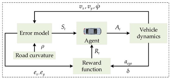
Figure 1. CF framework based on deep reinforcement learning.

The key to the training results’ quality lies in the design of the reward function, which transforms the FV’s longitudinal and lateral joint control problem into a multi-objective optimization problem of vehicle comfort, safety, yaw stability, and road traffic flow efficiency. To obtain a control strategy that meets the requirements of this article, the longitudinal speed, lateral speed, acceleration, lateral deviation, front wheel angle, the distance between two vehicles, and longitudinal speed error between them are constrained. According to various tests and the design principle of the reward function [24], the designed reward function is as follows:

$$r_t=-(0.1e_y^2+0.5{\delta }^2+0.01e_v^2+0.1a_{ego}^2)+2Y_t^2+V_t^2+D_t+E_t+F_t$$

(7)

$$Y_t=\left\{\begin{array}{l}2e_y^2\hspace{1em}{e}_y^2<0.01\hfill \\ 0\hspace{1em}\hspace{1em}otherwise\hfill \end{array}\right.,V_t=\left\{\begin{array}{l}{e}_v^2\hspace{1em}{e}_v^2<1\hfill \\ 0\hspace{1em}\hspace{1em}otherwise\hfill \end{array}\right.$$

(8)

$$D_t=\left\{\begin{array}{l}-10\hspace{1em}{e}_s<0\hfill \\ 0\hspace{1em}\hspace{1em}otherwise\hfill \end{array}\right.,E_t=\left\{\begin{array}{l}-10\hspace{1em}{v}_{ego}<0.1\hfill \\ 0\hspace{1em}\hspace{1em}otherwise\hfill \end{array}\right.,F_t=\left\{\begin{array}{l}-10\hspace{1em}\sigma (e_y)>1.5\hfill \\ 0\hspace{1em}\hspace{1em}otherwise\hfill \end{array}\right.$$

(9)

When any of the parameters in $D_t,E_t$ and $F_t$ are equal to −10, the training of the current episode will be terminated. As the training results begin to converge, the value $r_t$ gradually ascends, and the entire training process will stop until $r_t$ attains the preset value or the number of training times reaches the preset value.

As shown in Figure 2, the DDPG algorithm adopts the actor-critic framework. The input of the actor network is the observation $S_t$, and the output action $A_t$ is based on policy $\pi (s,a;\theta )$. The critic network is employed to estimate the value function $Q_t$ and uses this value function as the benchmark for updating the actor network. To diminish the influence of overestimation and bootstrapping, a target network is embedded in the actor-network and the critic network, respectively, to predict the action and the value of the state value function at the next moment. The actor and critic networks both contain a 5-layer network structure, including an input layer, three hidden layers, and an output layer, and each hidden layer contains 100 neurons [25].

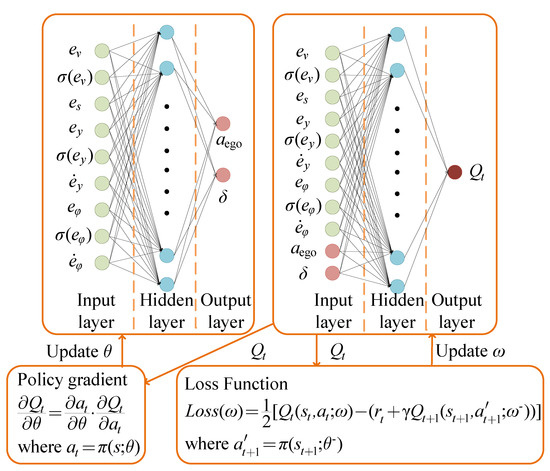
Figure 2. Network framework and parameter update of DDPG algorithm.

Policy is the probability distribution of taking action $a$ in state $s$:

$$\pi (s,a;\theta )=P\hspace{0.17em} [A_t=a|S_t=s\hspace{0.17em};\theta ]$$

(10)

The action value function is the cumulative discounted reward for taking action $a$ in state $s$ according to policy $\pi$:

$$Q_{\pi }(s,a;\omega )=E_{\pi }[{\displaystyle \sum _{k=0}^{\infty }{\gamma }^k}{R}_{t+k+1}|S_t=s,A_t=a]$$

(11)

When the policy is deterministic, then the state value function is:

$$Q_t=Q_t(s_t,a_t;\omega )=E_{A~\pi (·|s_t)}[{\displaystyle \sum _{k=0}^{\infty }{\gamma }^k}{R}_{t+k+1}|S_t=s]$$

(12)

The agent updates parameters and learns to make optimal actions according to the policy during the learning process by obtaining the maximum cumulative reward. Actor network updates network parameters $\theta$ based on gradient ascent:

$$\theta \leftarrow \theta +\mathsf{\beta }\cdot \frac{\partial a_t}{\partial \theta }\cdot \frac{\partial Q_t}{\partial a_t}$$

(13)

Use two target networks to predict the value function $Q_{t+1}^{\prime }$ and action $a_{t+1}^{\prime }$ at the next moment, respectively (Equation (14)). Then the temporal-difference error seen the Equation (15).

$$\left\{\begin{array}{l}{a}_{t+1}^{\prime }=\pi (s_{t+1}\hspace{0.17em};{\theta }^{-})\\ Q_{t+1}^{\prime }=Q(s_{t+1},a_{t+1}^{\prime };{\omega }^{-})\end{array}\right.$$

(14)

$${\xi }_t=Q_t-(r_t+\gamma Q_{t+1}^{\prime })$$

(15)

Critic network updates network parameter $\omega$ via a time-difference error:

$$\omega \leftarrow \omega -\alpha \cdot {\xi }_t\cdot \frac{\partial Q_t}{\partial \omega }$$

(16)

After each training, store the previous state transition sequence in the replay buffer as empirical data, and then update the actor and critic network parameters and two target network parameters, ${\omega }^{-}$ and ${\theta }^{-}$ (Equation (17)). The pseudo-code of the DDPG algorithm is shown in Algorithm 1.

$$\left\{\begin{array}{l}{\omega }^{-}\leftarrow \mathsf{\tau }\times \omega +(1-\mathsf{\tau })\times {\omega }^{-}\\ {\theta }^{-}\leftarrow \mathsf{\tau }\times \theta +(1-\mathsf{\tau })\times {\theta }^{-}\end{array}\right.$$

(17)

Algorithm 1 DDPG algorithm pseudo-code.

Car-Following Model Based on DDPG

Initialize$Q(s,a\hspace{0.17em};\omega )$$\mathrm{and} \pi (s,a\hspace{0.17em};\theta )$ with random weights ω and θ

Initialize the target network: $Q^{\prime }(s,a^{\prime }\hspace{0.17em};{\omega }^{-})\leftarrow Q(s,a\hspace{0.17em};\omega )$$,\pi (s,a^{\prime }\hspace{0.17em};{\theta }^{-})\leftarrow \pi (s,a\hspace{0.17em};\theta )$

Initialize Replay buffer

Forepisode = 1, M do

Initialize a random process for action exploration $\mathbb{N}$

receive initialization status $s_1$

For$t=1, T_f$ do

Choose action based on current policy and noise: $a_t=\pi (s_t\hspace{0.17em};\theta )+N_t$

Perform action $a_t$, get feedback rewards $r_t$ and move to the next state $s_{t+1}$

Store the state transition sequence $(s_t,a_t,r_t,s_{t+1})$ in the reply buffer

Randomly take a batch of samples from the replay buffer

Calculate $y_t=r_t+\gamma Q_{t+1}^{\prime }(s_{t+1},a_{t+1}^{\prime };{\omega }^{-})$ via the temporal-difference algorithm

Update the Critic network: $\mathit{Loss}\left(\omega \right)=\frac{1}{2}\left[Q_t\right(s_t,a_t;\omega )-y_t\left)\right]$

Update the actor network via gradient ascent: $\theta \leftarrow \theta +\mathsf{\beta }\cdot \frac{\partial a_t}{\partial \theta }\cdot \frac{\partial Q_t}{\partial a_t}$

Update target network: ${\omega }^{-}\leftarrow \mathsf{\tau }\times \omega +(1-\mathsf{\tau })\times {\omega }^{-}$$, {\theta }^{-}\leftarrow \mathsf{\tau }\times \theta +(1-\mathsf{\tau })\times {\theta }^{-}$

End for

End for

2.5. Car-Following Model Based on MADDPG

In 2017, OpenAI proposed a multi-agent deep deterministic policy gradient to improve the AC algorithm, which is suitable for complex multi-agent scenarios that traditional RL algorithms cannot handle [26]. As shown in Figure 3, the MADDPG model chooses a decentralized learning architecture. Each agent in the architecture is an independent individual with a separate policy network. It learns its policies through observations and reward values, and information cannot be shared. Therefore, the learning method of each agent is essentially the same as that of DDPG. Agent1 and Agent2 of the MADDPG model are respectively responsible for vertical and horizontal decision control. The reward functions are:

$$\left\{\begin{array}{l}{r}_t^{\left(1\right)}=-(0.1e_y^2+0.5{\delta }^2)+2Y_t^2+F_t\\ r_t^{\left(2\right)}=-(0.01e_v^2+0.1a_{ego}^2)+V_t^2+D_t+E_t\end{array}\right.$$

(18)

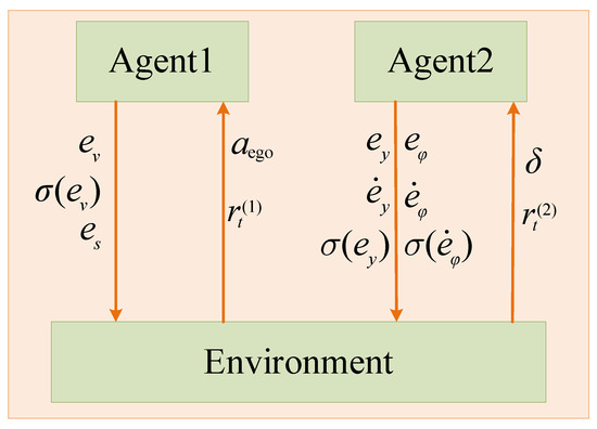
Figure 3. MADDPG CF model framework.

The network structure and parameter update method of a single agent in MADDPG are the same as those of DDPG and will not be repeated here. The training parameters are set as shown in Table 2.

Table 2. Deep reinforcement learning parameters.

Parameter	Symbol	DDPG	MADDPG
Sampling step	$T_s$ (s)	0.1	0.1
Training time per episode	$T_f$ (s)	60	60
Actor learning rate	$\alpha$	1 × 10−4	1 × 10−4
Critic learning rate	$\mathsf{\beta }$	1 × 10−3	1 × 10−3
Soft update rate	$\mathsf{\tau }$	1 × 10−3	1 × 10−3
Discount factor	$\gamma$	0.99	0.99
Replay buffer capacity	/	1 × 106	1 × 106
Batch size	/	64	64
Maximum training episode	/	3000	2000
Termination episode return value	/	1670	1670

2.6. Evaluation Metrics for Car-Following Behavior

The CF behavior is evaluated on four aspects: (1) safety; (2) comfort of CF; (3) road traffic flow efficiency; (4) lateral control effect of the FV. Safety is the most essential attribute in the CF process. The Time-To-Collision (TTC) is used to evaluate CF safety [27]. $\Delta S\left(t\right)$ is the gap between the two cars, and $\Delta v\left(t\right)$ is the velocity difference between the FV and the LV. For comparison, when TTC is less than 0, TTC equals −2.

$$TT\mathrm{C}(t)=\left\{\begin{array}{l}\frac{\Delta S(t)}{\Delta v(t)}\hspace{1em}\Delta v>0\hfill \\ -2\hspace{1em}\hspace{1em}\Delta v\le 0\hfill \end{array}\right.$$

(19)

Use the rate of change of acceleration to evaluate the comfort during CF (Equation (20)). The smaller the absolute value of Jerk, the smaller the impact and the higher the comfort.

$$Jerk(t)=\frac{a(t+\Delta t)-a(t)}{\Delta t}$$

(20)

Traffic flow efficiency can be evaluated by time headway (THW) (Equation (21)). From the literature [20], 1.2 s is selected as the danger threshold of the THW, and collisions are probably to occur below the danger threshold. Within the safe range, the shorter the THW, the better the tracking effect, and the higher the traffic flow efficiency [28].

$$THW(t)=e_s(t)/\frac{1}{n}{\displaystyle {\sum }_{t=0}^n{v}_{ego}(t)}$$

(21)

The lateral control effect is evaluated by lateral offset and yaw rate. The lateral offset is positively related to the control accuracy, and the yaw rate is positively associated with the lateral stability.

3. Results

A set of data of the lead vehicle is randomly selected and imported into the trained CF model for simulation verification in the database. The trajectory data generated by the DDPG and the MADDPG models are compared with the actual trajectory data.

3.1. Training Result

Figure 4 signifies the trend of reward changes in the training process of the CF model. The DDPG model fully meets the convergence requirements in about 2090 episodes, and the entire training time is 3 h 58 min; the MADDPG model is completed in about 800 episodes, and the whole training time is 2 h 19 min. The training time required for the MADDPG model is 41.59% less than that of the DDPG model, effectively reducing the training time cost.

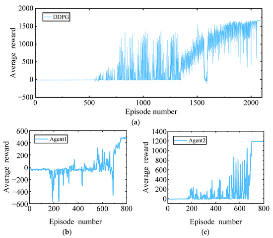
Figure 4. Training result: (a) DDPG; (b) Agent1 of MADDPG; (c) Agent2 of MADDPG.

3.2. Car-Following Effect on Straight Roads

Figure 5 shows the simulation results under straight road conditions. The Jerk values of the HDV and the vehicle under the control of the MPC model are mainly distributed at −1.4~1.3 m/s³ and −0.7~0.6 m/s³, respectively. In contrast, the Jerk values of the vehicle under the control of the MADDPG model and DDPG model are mainly distributed in −0.3~0.2 m/s³ and −0.2~0.2 m/s³, respectively. This indicates that the vehicle under the control of the DDPG model and the MADDPG model can weaken the frequency of acceleration and deceleration in the process of CF; additionally, the MADDPG model is more comfortable than the HDV and the vehicle under the control of the MPC model. Compared with the HDV, the vehicles under the control of the DDPG model and the MADDPG model always maintain a lower relative speed with the LV, which means that the TTC is longer and the safety is higher. The vehicles under the control of the MADDPG model and DDPG model have a more well-balanced following distance than the HDV. The THW of the vehicle under the control of the MADDPG model and DDPG model are respectively mainly distributed in the range of 1.2~1.6 s and 1.3~1.9 s, with high traffic flow efficiency under safe conditions. Although the THW distribution range of the vehicle under the control of the MPC model is 1.0~1.4 s, with the highest traffic efficiency, the proportion of THW below the safety threshold (1.2 s) is 48.5%, reducing the safety of car-following. The lateral offset of the vehicle under the control of the MADDPG model, the DDPG model, and the MPC model is less than that of the HDV, and the maximum value is decreased by 80.86%, 71.92%, and 85.71%, respectively. The yaw rate can be maintained near 0 after a short fluctuation, and the lateral stability is better than that of the HDV.

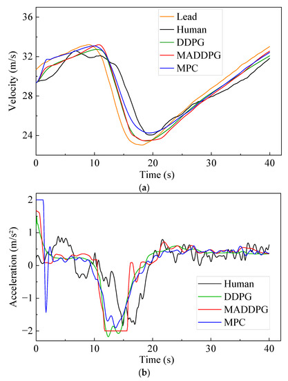
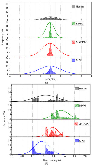
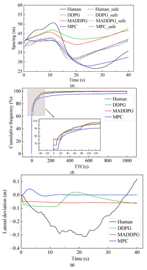
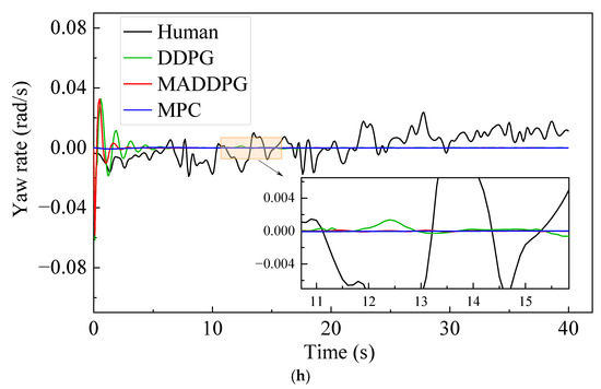
Figure 5. CF effect under straight road conditions: (a) speed; (b) acceleration; (c) distribution of Jerk; (d) distribution of THW; (e) following spacing; (f) distribution of TTC; (g) lateral offset of FV; (h) yaw rate of FV.

Figure 6 shows the simulation results under curve road conditions. The Jerk values of the HDV and the vehicle under the control of the MPC model are mainly distributed at −1.2~1.0 m/s³ and −1.2~1.8 m/s³, respectively. In contrast, the Jerk values of the vehicle under the control of the MADDPG model and DDPG model are mainly distributed in −0.5~0.5 m/s³ and −0.5~0.3 m/s³, respectively, indicating that the vehicle under the control of the DDPG model and the MADDPG model can still maintain better riding comfort than the HDV and the vehicle under the control of the MPC model. It can be seen from the TTC curve (Figure 6f) that, compared with the vehicle under the control of the DDPG model and the MADDPG model, the TTC values of the vehicle under the control of the MPC and HDV have an earlier turning point, which means that the MPC model and HDV have less negative TTC values, which means lower security (negative means that the two vehicles will never collide under the current state). The THW of the vehicle under the control of the MADDPG model and DDPG model are mainly distributed in the range of 1.28~1.42 s and 1.39~1.6 s, respectively, with high traffic flow efficiency under safe conditions. Although the THW distribution range of the vehicle under the control of the MPC model is 1.08~1.41 s, with the highest traffic efficiency, the proportion of THW below the safety threshold (1.2 s) is 49.40%, reducing the safety of car-following. The lateral offset of the vehicle under the control of the MADDPG model, the DDPG model, and the MPC model is less than that of the HDV, and the maximum value is decreased by 83.67%, 78.95%, and 87.95%, respectively. The yaw rate keeps a relatively stable state after a short fluctuation, and the lateral stability is better than that of the HDV.

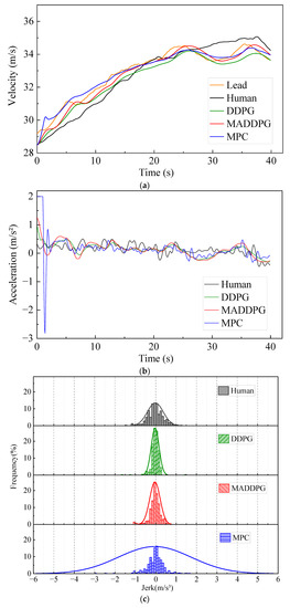
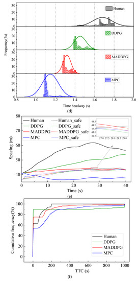
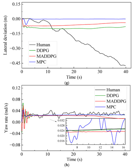
Figure 6. CF effect under linear, curved conditions: CF effect under linear road conditions: (a) speed; (b) acceleration; (c) distribution of Jerk; (d) distribution of THW; (e) following spacing; (f) distribution of TTC; (g) lateral offset of FV; (h) yaw rate of FV.

The simulation results show that, although the MPC car-following model is slightly better than the car-following model based on reinforcement learning in horizontal control, compared with the MPC model, the deep reinforcement learning model has the following advantages: (1) Under the same computer configuration and operating environment, the running time of the MADDPG model, DDPG model, and MPC model is 2.28 s, 2.42 s, and 11.31 s, respectively. This shows that the computational power required by the CF model based on deep reinforcement learning is significantly reduced compared with the MPC model (79.84% and 78.60%, respectively); (2) In terms of longitudinal control performance, it can be seen from the distribution of TTC, THW, and Jerk that the safety and comfort of MADDPG model and DDPG model are higher than those of MPC model.

4. Discussion and Conclusions

This study established the CF models based on the three degrees of freedom vehicle dynamics model and deep deterministic policy gradient algorithm. The reward function constrained the CF behavior’s safety, comfort, traffic flow efficiency, and lateral stability. The CF models were trained and validated using the OpenACC database, and the results reveal that the training time of the MADDPG model is 41.59% shorter than that of the DDPG model, which can save the expense of training time. The safety and comfort of the vehicle under the control of the MADDPG and DDPG models are higher than those of human-driven vehicles in straight and curved conditions. Since the drivers make an error in judging the following distance, it is uneasy to maintain a relatively stable following distance, resulting in a considerable THW of the human-driven vehicle and low road traffic flow efficiency. The THW of the vehicle under the control of the MADDPG model satisfies the safety preconditions with the smallest value and the highest road traffic flow efficiency. Compared with the human-driven vehicle, the vehicle under the control of the MADDPG and DDPG models can effectively decrease the maximum lateral offset and perk the lateral control accuracy. Due to the significant difference between the initial speed of the FV and the speed of the LV, the initial acceleration of the model is more prominent when the speed of the FV approaches the speed of the LV. Therefore, the yaw rate will gradually stabilize near the expected value after a brief fluctuation, which implies that the vehicle under the control of the MADDPG model and the DDPG model can significantly improve the lateral stability of the FV and effectively reduce the risk of car rollover. The following research can be expanded into the following aspects: (1) Consider combining lane-changing decisions with a car following to achieve more advanced intelligent driving; (2) The reward function can consider more constraints, such as fuel consumption.

References

- Wang, W.; Wang, Y.; Liu, Y.; Wu, B. Headway Distribution Considering Vehicle Type Combinations. J. Transp. Eng. Part A-Syst. 2022, 148, 04021119. [Google Scholar] [CrossRef]
- Zong, F.; Wang, M.; Tang, M.; Li, X.; Zeng, M. An improved intelligent driver model considering the information of multiple front and rear vehicles. IEEE Access. 2021, 9, 66241–66252. [Google Scholar] [CrossRef]
- Yu, Y.; Jiang, R.; Qu, X. A modified full velocity difference model with acceleration and deceleration confinement: Calibrations, validations, and scenario analyses. IEEE Intell. Transp. Syst. Mag. 2019, 13, 222–235. [Google Scholar] [CrossRef]
- Ardakani, M.K.; Yang, J. Generalized Gipps-type vehicle-following models. J. Transp. Eng. Part A-Syst. 2017, 143, 04016011. [Google Scholar] [CrossRef]
- He, Y.; Montanino, M.; Mattas, K.; Punzo, V.; Ciuffo, B. Physics-augmented models to simulate commercial adaptive cruise control (ACC) systems. Transp. Res. Pt. C-Emerg. Technol. 2022, 139, 103692. [Google Scholar] [CrossRef]
- Meng, D.; Song, G.; Wu, Y.; Zhai, Z.; Yu, L.; Zhang, J. Modification of Newell’s car-following model incorporating multidimensional stochastic parameters for emission estimation. Transport. Res. Part D-Transport. Environ. 2021, 91, 102692. [Google Scholar] [CrossRef]
- Liu, Y.; Zou, B.; Ni, A.; Gao, L.; Zhang, C. Calibrating microscopic traffic simulators using machine learning and particle swarm optimization. Transp. Lett. 2021, 13, 295–307. [Google Scholar] [CrossRef]
- Gao, K.; Yan, D.; Yang, F.; Xie, J.; Liu, L.; Du, R.; Xiong, N. Conditional artificial potential field-based autonomous vehicle safety control with interference of lane changing in mixed traffic scenario. Sensors 2019, 19, 4199. [Google Scholar] [CrossRef]
- Qu, D.; Wang, S.; Liu, H.; Meng, Y. A Car-Following Model Based on Trajectory Data for Connected and Automated Vehicles to Predict Trajectory of Human-Driven Vehicles. Sustainability 2022, 14, 7045. [Google Scholar] [CrossRef]
- Li, W.; Zhang, Y.; Shi, X.; Qiu, F. A Decision-Making Strategy for Car Following Based on Naturalist Driving Data via Deep Reinforcement Learning. Sensors 2022, 22, 8055. [Google Scholar] [CrossRef]
- Ye, Y.; Zhang, X.; Sun, J. Automated vehicle’s behavior decision making using deep reinforcement learning and high-fidelity simulation environment. Transp. Res. Pt. C-Emerg. Technol. 2019, 107, 155–170. [Google Scholar] [CrossRef]
- Zhang, D.; Li, K.; Wang, J. A curving ACC system with coordination control of longitudinal car-following and lateral stability. Veh. Syst. Dyn. 2012, 50, 1085–1102. [Google Scholar] [CrossRef]
- Zhang, J.; Li, Q.; Chen, D. Integrated Adaptive Cruise Control with Weight Coefficient Self-Tuning Strategy. Appl. Sci. 2018, 8, 978. [Google Scholar] [CrossRef]
- Chen, K.; Pei, X.; Okuda, H.; Zhu, M.; Guo, X.; Guo, K.; Suzuki, T. A hierarchical hybrid system of integrated longitudinal and lateral control for intelligent vehicle. ISA Trans. 2020, 106, 200–212. [Google Scholar] [CrossRef] [PubMed]
- Ghaffari, A.; Gharehpapagh, B.; Khodayari, A.; Salehinia, S. Longitudinal and lateral movement control of car following maneuver using fuzzy sliding mode control. In Proceedings of the 2014 IEEE 23rd International Symposium on Industrial Electronics, Istanbul, Turkey, 1–4 June 2014; IEEE: New York, NY, USA, 2014; pp. 150–155. [Google Scholar]
- Guo, J.; Luo, Y.; Li, K. Integrated adaptive dynamic surface car following control for nonholonomic autonomous electric vehicles. Sci. China-Technol. Sci. 2017, 60, 1221–1230. [Google Scholar] [CrossRef]
- Yang, Y.; Ma, F.; Wang, J.; Zhu, S.; Gelbal, S.Y.; Kavas-Torris, O.; Guvenc, L. Cooperative ecological cruising using hierarchical control strategy with optimal sustainable performance for connected automated vehicles on varying road conditions. J. Clean. Prod. 2020, 275, 123056. [Google Scholar] [CrossRef]
- Li, Y.; Chen, W.; Peeta, S.; Wang, Y. Platoon Control of Connected Multi-Vehicle Systems Under V2X Communications: Design and Experiments. IEEE Trans. Intell. Transp. Syst. 2020, 21, 1891–1902. [Google Scholar] [CrossRef]
- Lin, Y.; McPhee, J.; Azad, N.L. Comparison of Deep Reinforcement Learning and Model Predictive Control for Adaptive Cruise Control. IEEE Trans. Intell. Veh. 2021, 6, 221–231. [Google Scholar] [CrossRef]
- Makridis, M.; Mattas, K.; Anesiadou, A.; Ciuffo, B. OpenACC. An open database of car-following experiments to study the properties of commercial ACC systems. Transp. Res. Pt. C-Emerg. Technol. 2021, 125, 103047. [Google Scholar] [CrossRef]
- Wang, Y.; Ding, H.; Yuan, J.; Chen, H. Output-feedback triple-step coordinated control for path following of autonomous ground vehicles. Mech. Syst. Signal. Proc. 2019, 116, 146–159. [Google Scholar] [CrossRef]
- Puan, O.C.; Mohamed, A.; Idham, M.K.; Ismail, C.R.; Hainin, M.R.; Ahmad, M.S.A.; Mokhtar, A. Drivers behaviour on expressways: Headway and speed relationships. In IOP Conference Series: Materials Science and Engineering; IOP Publishing: Bristol, UK, 2019; Volume 527, p. 012071. [Google Scholar]
- Lillicrap, T.P.; Hunt, J.J.; Pritzel, A.; Heess, N.; Erez, T.; Tassa, Y.; Silver, D.; Wierstra, D. Continuous control with deep reinforcement learning. arXiv 2015, arXiv:1509.02971. [Google Scholar]
- Sutton, R.S.; Barto, A.G. Reinforcement Learning: An Introduction; MIT Press: Cambridge, MA, USA, 2018. [Google Scholar]
- Zhu, M.; Wang, X.; Wang, Y. Human-like autonomous car-following model with deep reinforcement learning. Transp. Res. Pt. C-Emerg. Technol. 2018, 97, 348–368. [Google Scholar] [CrossRef]
- Lowe, R.; Wu, Y.I.; Tamar, A.; Harb, J.; Pieter Abbeel, O.; Mordatch, I. Multi-agent actor-critic for mixed cooperative-competitive environments. In Proceedings of the 31st Conference on Neural Information Processing Systems (NIPS 2017), Long Beach, CA, USA, 4–9 December 2017; Volume 30. [Google Scholar]
- Pu, Z.; Li, Z.; Jiang, Y.; Wang, Y. Full Bayesian Before-After Analysis of Safety Effects of Variable Speed Limit System. IEEE. Trans. Intell. Transp. Syst. 2021, 22, 964–976. [Google Scholar] [CrossRef]
- Zhang, G.; Wang, Y.; Wei, H.; Chen, Y. Examining headway distribution models with urban freeway loop event data. Transp. Res. Record. 2007, 1999, 141–149. [Google Scholar] [CrossRef]
Publisher’s Note: MDPI stays neutral with regard to jurisdictional claims in published maps and institutional affiliations. |
© 2022 by the authors. Licensee MDPI, Basel, Switzerland. This article is an open access article distributed under the terms and conditions of the Creative Commons Attribution (CC BY) license (https://creativecommons.org/licenses/by/4.0/).