A Sustainable Production Scheduling with Backorders under Different Forms of Rework Process and Green Investment

Abstract

Rework is currently a necessity for businesses and commercial organizations across the world. It is only beneficial in tackling climate change if the process emits less greenhouse gases than would otherwise be emitted. This study designs an optimal production scheduling model to reduce both carbon emissions during the processes of production, transport and storage, and setup cost by leveraging on green technology efforts in an imperfect production process where a fraction of items is erroneous so that the firm may run out of inventory. The producer implements a rework strategy to rectify the flawed products, anda flexible rework rate is offered since the rework might be executed on various schemes. The flexible rework allows the producer to choose therework rate, which can differ from the production rate, as well as the rework process itself, which can be asynchronous or synchronous.The two forms of green investments: quadratic and exponential are considered in the study. The main point of the study is to derive a solution procedure of the various problem settings associated with the rework rate, rework process and green investment. The findings suggest that developing the optimal production schedule (lot-sizes, backorders, setup cost and green investment amount) can lower the manufacturing sector’s excessive ecological carbon emissions. The findings also support the idea that making green investments is the most cost-effective way to cut carbon emissions and setup cost simultaneously.

1. Introduction

The Economic Production Quantity (EPQ) inventory techniqueis one of the most vital approaches in the manufacturing system for managing production since it notifies the producer when to halt production and use the products in inventory to meet consumer demand. The EPQ is based on the assumption that the company will create its own quantity or that the components will be delivered to the company as they are built, allowing orders to be available or received incrementally while the products are being produced. A shortage occurs when demand for a product or service exceeds available supply. This is a transitory state since the item will be restocked, and the market will return to balance. Unfortunately, no factory’s production is perfect. Product faults abound in the manufacturing industry. They are available in a range of shapes and sizes. Moreover, they are an issue that might have a significant influence on their bottom line as an importer. As a result, we expect to diminish the amount of faulty goods by modifying them.

Product rework plays a critical role in the execution of the retail inventory system. It is a word that refers to the processes needed to alter or repair items in order to satisfy a firm’s inventory needs.Rework of a product may be necessary by businesses to address real or perceived quality concerns through adjustments or repairs to a product. For instance, an imported product may have entered the country and included mold that has to be cleaned. There could have been a production error in other cases.Examples of product errors include sewing alterations or corrections, refinishing footwear to meet a brand’s color and finish designs, and replacement of poor-quality hardware or incorrect components on a shipment of finished goods. Therefore, product rework may be a crucial function to use to succeed in our supply chain execution tactic as we fulfill demands for inventory availability, regardless of whether a firm is an importer or an exporter of items.

Costs are another inevitable aspect ofthe inventory system. The long-term goal of cost reduction is to reduce costs without compromising the quality of the product. It is a technique to make a company’s operations more effective. Every organization benefits from a small upfront investment to reduce setup and problematic production costs. Due to a significant opening expenditure used to support upgraded machinery and other measures to improve the system, each individual setup cost is decreased and the quantity of defective items is reduced.

The third stream of the literature related to our model is carbon emissions (CO₂). The literature in this stream is vast. The main cause of global warming today is the greenhouse gas impact, which is brought on by growing pollution levels. About 1/5th of greenhouse gas CO₂ comes from manufacturing, food processing, mining, and building. Numerous activities result in direct CO₂, such as the on-site burning of fossil fuels for heat andelectricity, the use of fossil fuels for purposes other than energy, and chemical processes involved in the production of iron, steel, and cement. Industry emits indirect CO₂ as a result of the centrally generated power it uses. The industrial sector accounts for around one-quarter of overall power sales. The burning of fossil fuels generates energy and heat, and transportation is the largest source of CO₂ in the atmosphere (Source: Annual Energy Outlook 2021). Figure 1 depicts this. The industrial segment may reduce greenhouse gas CO₂ in a number of methods, including energy efficiency, fuel shifting, combined heat and power, renewable energy, green investment, carbon tax, more efficient raw material utilization, and recycling. Green investments are business ventures that concentrate on areas of environmental protection, such as strategies for reducing pollution. Many industrial operations do not have a low-CO₂ alternative, necessitating long-term CO₂ capture and storage to minimize CO₂. Green technology, when applied correctly, has the potential to have a moral influence in terms of CO₂ reduction.

Resource conservation and efficiency are ensured through sustainable industrialdevelopment. Producers must analyze how raw materials are mined, components are made, products are created, and return markets are structured in order to optimize the supply chain and increase resource productivity. Think about innovative business models that would give us more control over every aspect of our operations to ensure that we are practicing environmental safety. The reducedecological effect through pollution avoidance is one of the most crucial elements of sustainability. Waste produces pollution, which can be avoided, repurposed, or decreased to provide environmental protection. There areseveral financial advantages to sustainable industrial growth. The sector itself promotes the employment and revenue opportunities connected to lessening ecological impacts. Additionally, sustainable industrial growth may help firms cut operational expenses. Processes that are efficient and sustainable require less energy, water, and materials, which may save a lot of money. The reducedecological impact is possibly the most evident benefit of sustainable industrialization. Many industrial firms are moving toward ecologically friendly development in order to conserve their ethical agreement to guarantee a safer and cleaner ecosystem. Sustainable industrial development aims to reduce greenhouse gas CO₂ while conserving natural resources.

1.1. Literature Review

Rosenblatt and Lee [1] invented an EPQ model for a flawed production procedure with a constant, linear, exponential, or multistate defective rate. Later, a number of scholars extended Rosenblatt and Lee’s [1] work witha variety of hypotheses (see [2,3,4,5,6,7,8,9]), and all of these models utilize a method for removing damaged products once they are detected. Rather than being discarded, broken products are recovered and used as raw materials in everyday production. In view of this, Liu and Yang’s [10] EPQ model argues that a flawed manufacturing system can create damaged items that are both reworkable and non-reworkable. Hayek and Salameh [11] estimated the manufacturing lot-size when shortages are granted, and the portion of spoiled goods is a random variable.

Liao et al. [12,13] evaluated the EPQ and optimal preemptive upkeep schedule for inadequate production activity including the rework of damaged goods. Krishnamurthy et al. [14] extended an EPQ model withaproblematic manufacturing structure to include frequent manufacturing rework and sales returns. After production, defective items are detected and reworked. If manufacturing demands are unique, production planning may be a challenge. In the case of defective production, for example, requirements may vary with the amount of stock; this issue is examined and appraised in [15]. Repairingdamaged items may be conductedin two ways: after-producing rework and during-producing rework. Rework of items and manufacturingare considered synchronous operations, but the rework of faulty goods after production is considered asynchronous. Nihar et al. [16] implied the requirement of taking the synchronous and asynchronous decision-making activities of diverse inventory systems. They studied how the various synchronous and asynchronous functions affect the system’s actions. Al-Salamah [17] formed an EPQ inventory model with synchronous and asynchronous variable rework rates to account for an imperfect manufacturing process. He offered two configurations for the rework process. Imperfect components may only be modified utilizing the asynchronous rework option after the entire lot has been formed.Instead, with synchronous rework, damaged items may be repaired as soon as they are made.

Coates et al. [18] derived a method for lowering the cost of product setup in industries. Sarkar and Moon [19] created a quality improvement model with a variable setup cost and backorder rate using the concept of Porteus [20]. Lung Hou [21] established an EPQ model that included capital expenditure which is a function of setup cost and process quality. For the EPQ model with flaws, Freimer et al. [22] calculated the worth of setup cost reduction optimization. To decrease the setup in production systems with work-in-process inventories, Nye et al. [23] adopted an optimum investment. Sarkar et al. [24] designed a setup cost reduction inventory model with quality upgrading. Then, Tiwari et al. [25] studied an integrated multi-echelon inventory system whose coordination is hampered by quality concerns and human error. By conductingan early investment in the vendor’s manufacturing amenities, the buyer is prepared to minimize the vendor’s set-up costs.

Different sustainable strategies to reduce CO₂ have been established by the carbon regulating bodies in many industrialized nations. The main sustainable approaches are limited CO₂, carbon taxation, carbon cap and trade, and Green Lean Six Sigma (GLSS) which are often adopted by governments and private industries. In this connection, Bouchery et al. [26] explored traditional inventory procedures while analyzing the approach ofsustainability. They highlighted how CO₂ was slashed to a single goal function in terms of sustainable growth. Benjaafar et al. [27] created a model based on the cost function and CO₂ footprint by connecting CO₂ quantities to a variety of decision criteria. They were able to broaden their stance on CO₂ cut by making small operational changes, such as investing in green technologies. Toptal et al. [28] explored a joint inventory strategy with three unique CO₂ investment policies. Dye and Yang [29] investigated a trade-creditinventory system that included issues ondemand sustainability depending on credit terms. They discussed how credit duration and environmental restrictions influence the inventory model in the context of a CO₂ levy and cap system, with default risk rates. Qin et al. [30] developed a trade-credit inventory model for a CO₂ tax, a CO₂ cap, anda demand-based trade strategy under credit-period demand. Then, Datta [31] analyzed the effect of green investment to reduce CO₂ in an EPQ model. Following that, Huang et al. [32] derived a supply chain system that considered logistics, green investment, and various CO₂ norms. Mishra et al. [33] developed a long-term production-inventory model to reduce CO₂ when resources are scarce. Hasanet al. [34] figured out how to maximize inventory levels and technical investment withdifferent CO₂ strategies. We notice that the aforesaid papers considered the first three sustainable approaches. Despite rising curiosity about GLSS, only a small amount of research has been conductedon its use, and there has been no research conductedon the obstacles that prevent GLSS from being employed. The reduction in GLSS implementation hurdles in the industrial sector was examined by Kaswan et al. [35] based on their interaction with one another. Then, Kaswanet al. [36] proposed a GLSS implementation framework for enhanced organizational performance.The selection of the GLSS project for the industrial sector in the dynamic decision-making ecosystem is the focus of the study. Rathi et al. [37] also recently created a systematic GLSS framework for increasing operational effectivenesstogether with social and environmental sustainability. The framework, which covers the systematic application of numerous Green paradigm, Lean, and Six Sigma techniques from the identification and evaluation of the problem to the maintenance of the realized measures, was created with perceptions learned from the literature and industrial people. Mohan et al. [38] offered an analysis of GLSS research focused on a systematic literature study and expedited the organization’s readiness to apply sustainable GLSS practice via deep knowledge of realization.

1.2. Research Gaps and Contributions

The majority of studies in the collection of imperfect production were designed with reworks, repairs, etc. Although synchronous and asynchronous rework processes were studied by a few scholars, sustainable EPQ CO₂ tax and cap models of optimizing setup cost and CO₂ simultaneously under bothaforementioned rework processes are notaccessible. We enhance Al Salamah’s [17] approach in order to reduce setup costs and control CO₂ since the presence of CO₂ and cost reductions in setup make the model more realistic. The overview of the literature is given in

Table 1. Literature overview.

Author(s)	Rework	Synchronous and Asynchronous	Setup Cost Reduction	Backorders	CO2	Green Investment
Hsu et al. [4]				✓
Taleizadeh et al. [5]	✓			✓
Hsu et al. [6]				✓
Ganesan et al. [7]
Sujit et al. [8]	✓			✓
Liu et al. [10]	✓			✓
Hayek et al. [11]	✓
Liao et al. [12]	✓
Liao et al. [13]	✓
Krishnamurthy et al. [14]	✓			✓
Shah et al. [15]	✓
Nihar et al. [16]	✓	✓
Al-Salamah [17]	✓	✓		✓
Sarkar et al. [19]			✓
Ouyang et al. [39]			✓
Hou et al. [21]	✓		✓
Freimer et al. [22]			✓
Nye et al. [23]			✓
Tiwari et al. [25]			✓
Bouchery et al. [26]					✓
Benjaafar et al. [27]					✓
Toptal et al. [28]					✓	✓
Dye et al. [29]					✓
Qin et al. [30]					✓
Datta [31]					✓
Huang et al. [32]					✓	✓
Mishra et al. [33]					✓	✓
Kaswan et al. [36]					✓	✓
This paper	✓	✓	✓	✓	✓	✓

. In comparison to earlier studies, our study made the following contributions: This research takes into account a flawed production system with two rework processes. Previously published studies avoided the availability of green technologies to manage CO₂ and setup costs at the same time. According to Porteus [20], a logarithmic expression may be utilized to lessen the setup cost, and two distinct types of CO₂ reduction functions for green technology are being investigated to reduce CO₂.

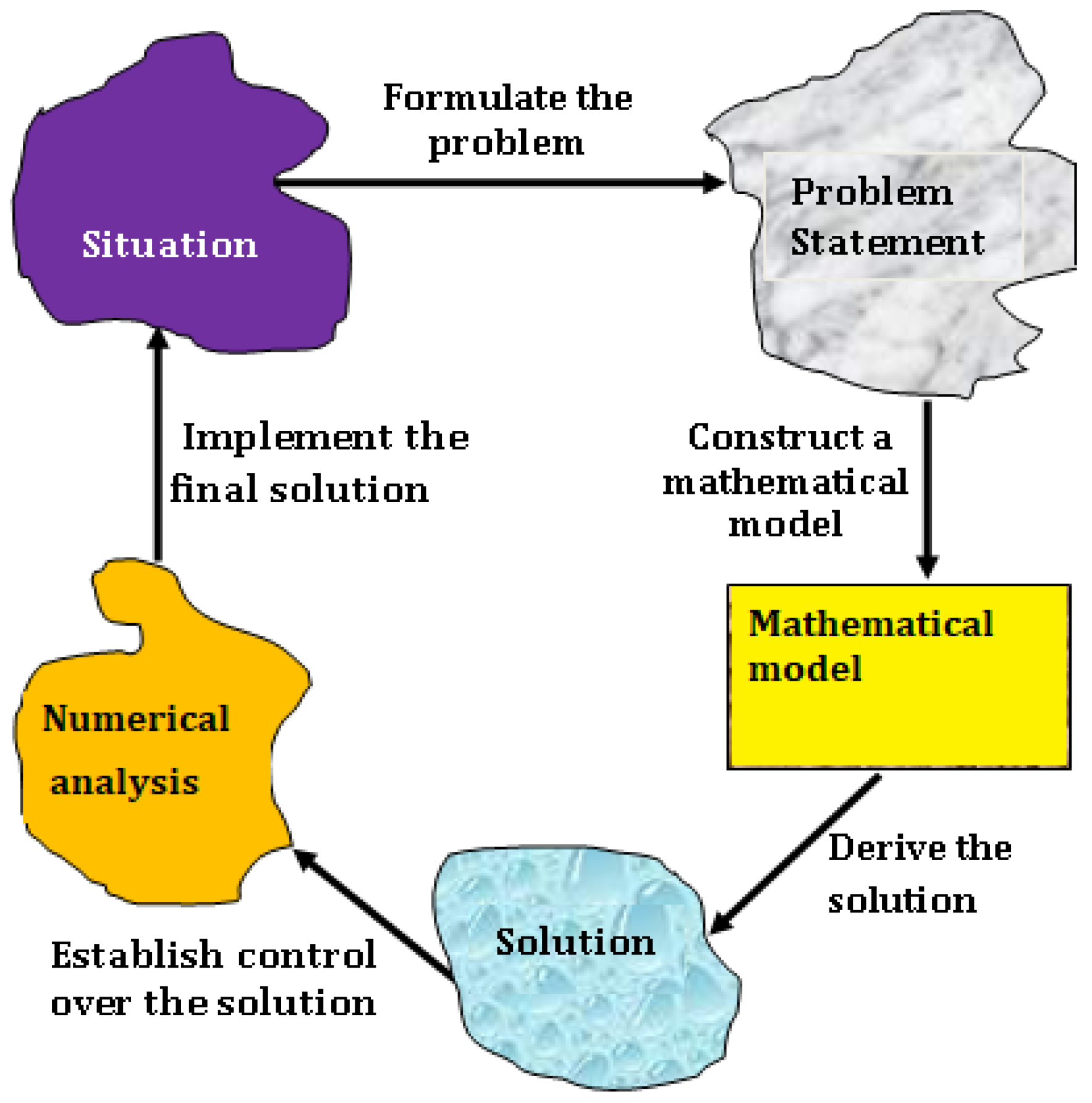
1.3. Research Methodology

The models in this study are based on mathematically oriented inventory theory, and the methodology used is the quantitative method, which is based on the principles of operations research and management science.The schematic diagram of the methodology is shown in Figure 2. In this study, we develop mathematical models and use differential calculus optimization techniques to find the optimal solutions forthe models. The methodology followed in this research to find the optimal production scheduling (lot-sizes, backorders, setup cost and green investment amount) is listed below:

• Description of the problem
• Mathematical model formulation
• Solution procedure
• Numerical Analysis

The rest of the study is designed in the same way: Section 2 shows the research’s required notations and assumptions. Section 3 and Section 4 formulate the mathematical models along with solution techniques. The sensitivity and numerical analysis are discussed in Section 5. Section 6 concludes the paper.

2. Descriptions of Problem

A producer creates inventory items in a flawed production system in order to supply customer-ordered quantities. A 100% inspection is performed to classify the problematic parts, which are stored apart from faultless ones and remodeled separately. The rework rate is variable and different from the manufacturing rate, and the rework activity can be synchronous or asynchronous. We examine CO₂ and extreme setup costs as a result of the system’s many industrial processes. The company intends to shift toward a greener production system by investing in modern technology, energy-efficient equipment, setup costs, non-traditional energy, and other elements. The amount of money that may be invested appears to be limited. The producer’s budget for the green technology renovation venture is denoted by this ceiling. With the producer’s approval, the back-ordering of shortage items is also feasible. The mathematical models were developed using the following assumptions and notations.

Assumptions

• Consumer requirement(demand) and production rate are constant.
• CO₂ are generated from the process of production, transportation, and storage.
• There are two primary forms that green technology might reduce CO₂:

  (i)

  $R_1 \left(G\right)=\alpha G-\beta G^2$, where $\alpha$ stands for the offsetting CO₂ reduction factor and $\beta$ for the CO₂ reduction efficiency factor (Huang et al. [32]).

  (ii)

  $R_2\left(G\right)=\xi \left(1-e^{-mG}\right)\Rightarrow G=-\left(\frac{1}{m}\right)\left[\ln \left(1-\frac{F}{\xi }\right)\right]$ where $m$ stands for the effectiveness of greener technology in decreasing CO₂, $\xi$ is a proportion of CO₂ after investment in green technology, and F is a fraction of average CO₂ reduction (Mishra et al. [33]).

• The relationship between setup cost reduction and capital investment may be defined using the logarithmic investment cost function. Therefore, S and the capital expenditure for S reduction ($\mathsf{\Pi }$) may be recorded as $\mathsf{\Pi }\left(S\right)=Mln\left(\frac{S_0}{S}\right)$ for $0<S\le S_0$ where $M=1/\delta$,$\delta$ is the fractional cut in S\dollar rise in $\Pi \left(S\right)$.

3. Production Scheduling with Asynchronous Rework

Due to the accumulation and rework of defective items occurring only after the manufacturing lot is ended, the production and rework processes are not synchronized. Due to the adaptability of rework and the potential for manufacturer-dependent variations, there are two options to take into account. The inventory curvature will have a positive slope if perfect inventory accumulates during $T_2$ as a result of $P_R$ being larger than D. However, if $P_R$ is less than D, the inventory of the perfect items constantly drops over $T_2$, resulting in a negative slope on the inventory curve for the perfect goods.In the next subsections, we examine each circumstance separately and compute the optimal $Q$, $S$, $B$, and $G$ for each type of green investment.

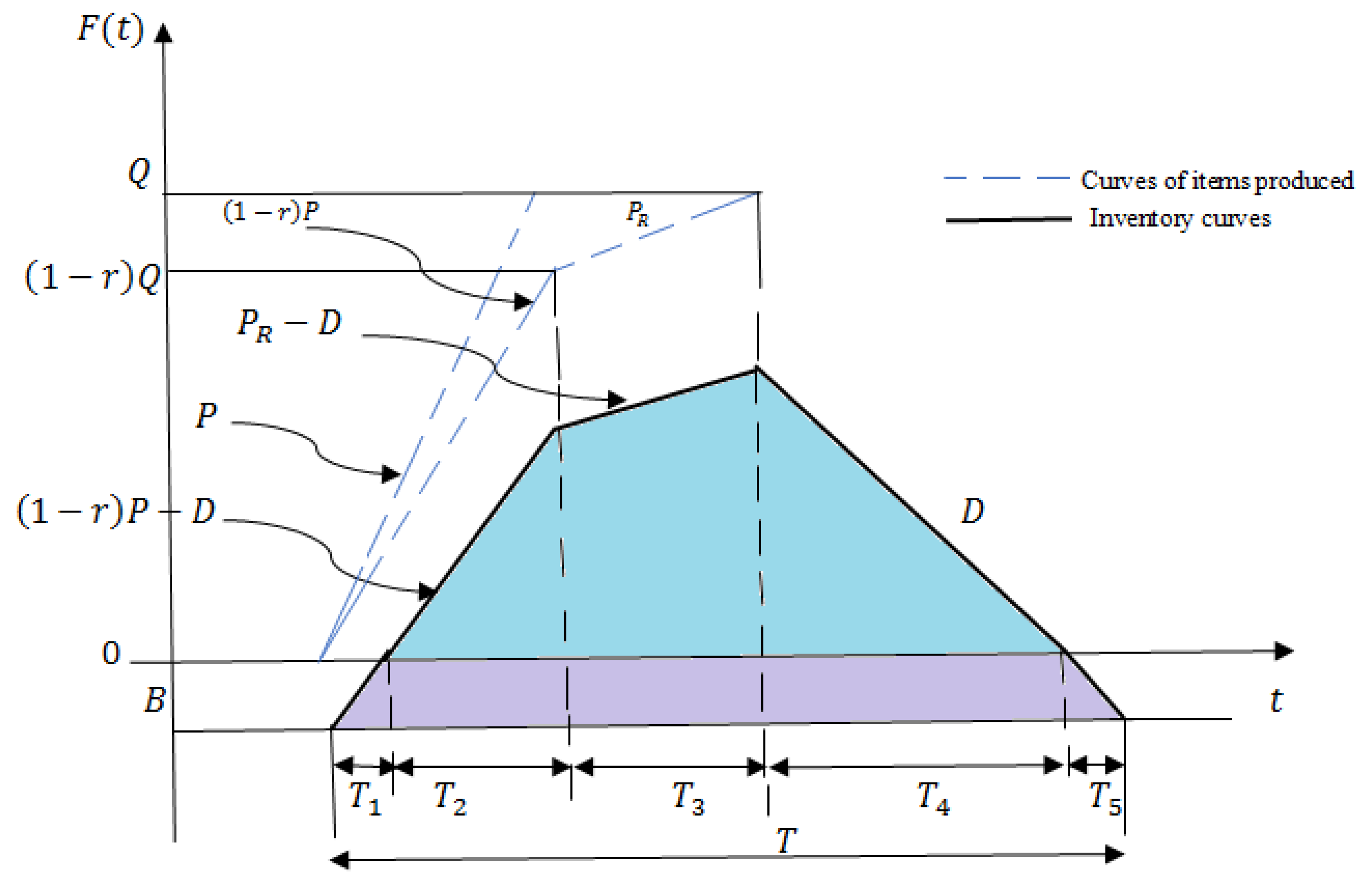
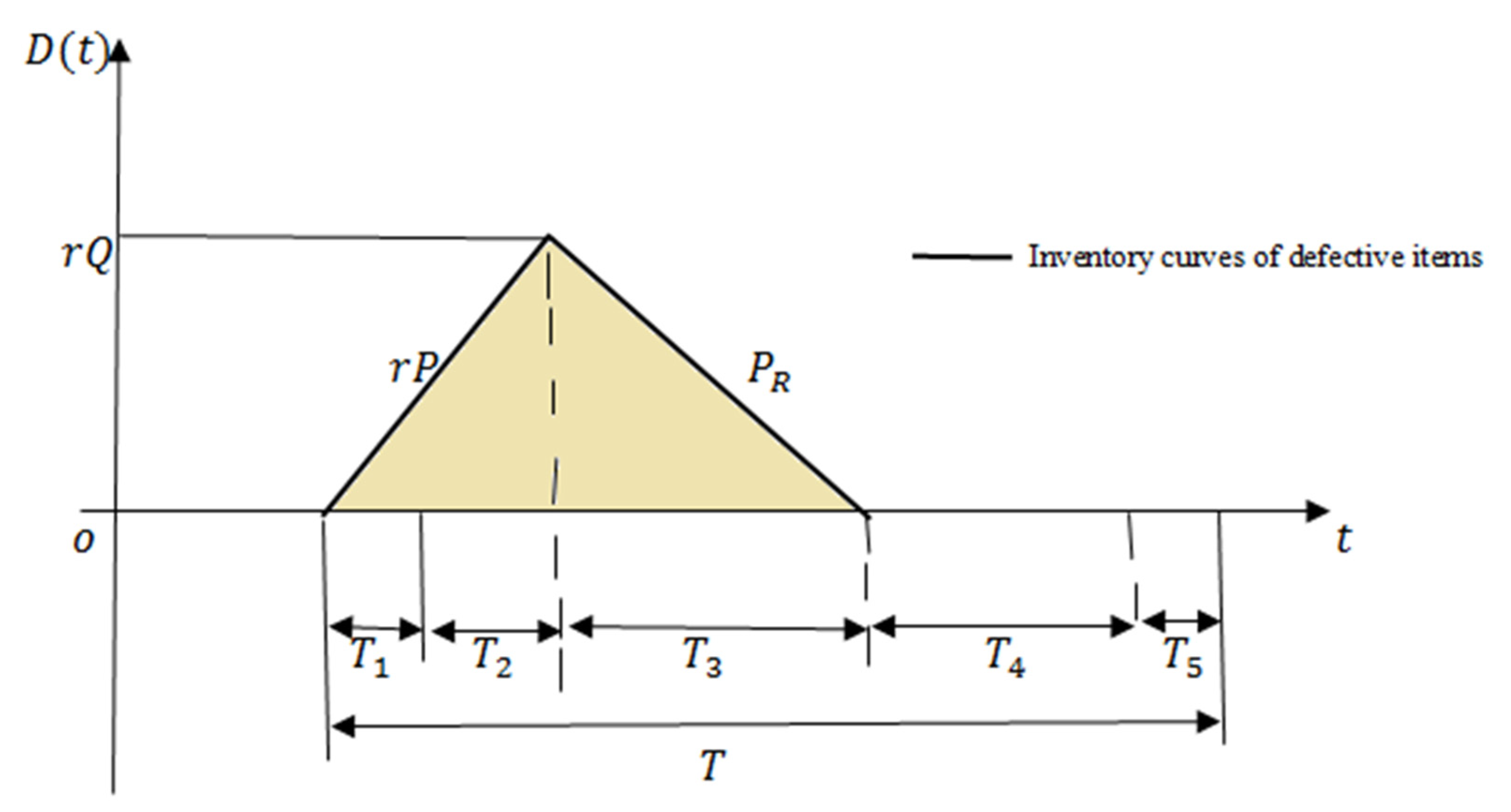
3.1. The P_R Is Higher than D (P_R > D)

The following can be calculated from Figure 3, which depicts the inventory curve of perfect items in a cycle with backorders.

The curve of back-order is $B_1\left(t\right)=\left[\left(1-r\right)P-D\right]t$with the initial conditions $B_1\left(0\right)=0$ and $B_1\left(T_1\right)=B$ during$T_1$. Hence, $B_1\left(T_1\right)=\left[\left(1-r\right)P-D\right]T_1$ implies $T_1=\frac{B}{\left(1-r\right)P-D}$. The total backorder quantities during $T_1$ is provided by ${{\displaystyle \int }}_0^{T_1}{B}_1\left(t\right)dt=\frac{B^2}{2\left[\left(1-r\right)P-D\right]}$.

During the production period $T_1+T_2$, the $Q$ units of products produced. That is, $\left(T_1+T_2\right)P=Q$. Then $T_2=\frac{Q}{P}-T_1=\frac{Q}{P}-\frac{B}{\left(1-r\right)P-D}$.

The inventory curve is $F_1\left(t\right)=B_1\left(t\right)$ during $T_2$. Then the total amount of inventory during $T_2$ is condcutedby ${{\displaystyle \int }}_0^{T_2}{F}_1\left(t\right)dt=\frac{1}{2}\left(\left(1-r\right)P-D\right){\left(\frac{Q}{P}-\frac{B}{\left(1-r\right)P-D}\right)}^2={\Pi }_0\left(Q,B\right)$.

The period $T_3$ is the time of rework $rQ$ items, and $T_3=\frac{rQ}{P_R}$ since the rework rate is $P_R$. For the period $T_3$, the inventory curve is $F_2\left(t\right)=\left(P_R-D\right)t+\left(\left(1-r\right)P-D\right)T_2$ with the initial condition $f_2\left(0\right)=f_1\left(T_2\right)=\left(\left(1-r\right)P-D\right)T_2$. Then the total inventory during $T_3$ is ${{\displaystyle \int }}_0^{T_3}{F}_2\left(t\right)dt=\frac{1}{2}\left(P_R-D\right){\left(\frac{rQ}{P_R}\right)}^2+\left(\left(1-r\right)P-D\right)\left(\frac{Q}{P}-\frac{B}{\left(1-r\right)P-D}\right)\left(\frac{rQ}{P_R}\right)$.

The inventory curve is ${\mathrm{F}}_3\left(\mathrm{t}\right)=\mathrm{Dt}$ with the end value ${\mathrm{F}}_3\left({\mathrm{T}}_4\right)={\mathrm{F}}_2\left({\mathrm{T}}_3\right)=\left({\mathrm{P}}_{\mathrm{R}}-\mathrm{D}\right){\mathrm{T}}_3+\left(\left(1-\mathrm{r}\right)\mathrm{P}-\mathrm{D}\right){\mathrm{T}}_2{ \mathrm{during} \mathrm{T}}_4$. The ${\mathrm{T}}_4$ can be derived as ${\mathrm{T}}_4=\frac{\left({\mathrm{P}}_{\mathrm{R}}-\mathrm{D}\right){\mathrm{T}}_3+\left(\left(1-\mathrm{r}\right)\mathrm{P}-\mathrm{D}\right){\mathrm{T}}_2}{\mathrm{D}}=\frac{\mathrm{Q}}{\mathrm{D}}-\frac{\mathrm{B}}{\mathrm{D}}-\frac{\mathrm{Q}}{\mathrm{P}}-\frac{\mathrm{rQ}}{{\mathrm{P}}_{\mathrm{R}}}$ from the terminal value.

The total inventory during ${\mathrm{T}}_4$ is ${{\displaystyle \int }}_0^{{\mathrm{T}}_4}{\mathrm{F}}_3\left(\mathrm{t}\right)\mathrm{dt}=\frac{1}{2}\mathrm{D}{\left(\frac{\mathrm{Q}}{\mathrm{D}}-\frac{\mathrm{B}}{\mathrm{D}}-\frac{\mathrm{Q}}{\mathrm{P}}-\frac{\mathrm{rQ}}{{\mathrm{P}}_{\mathrm{R}}}\right)}^2$.

The function of backorder quantities is $B_2\left(t\right)=Dt$ with terminal value is $B_2\left(T_5\right)=B$ during $T_5=\frac{B}{D}$. Hence, during $T_5$, the total backorder is ${{\displaystyle \int }}_0^{T_5}{B}_2\left(t\right)dt=\frac{1}{2}\frac{B^2}{D}$.

Next, we evaluate the inventory, which is depicted in Figure 4 as a curve of flawed items with asynchronous rework. The following can be deduced from Figure 4.

During the period $T_1+T_2$, the inventory curve of flawed items is $D_1\left(t\right)=rPt$ with the terminal value $D_1\left(T_1+T_2\right)=rP\left(T_1+T_2\right)=rQ$. Since $T_1+T_2=\frac{Q}{P},$ the total inventory of the flawed products during $T_1+T_2$ is ${{\displaystyle \int }}_0^{T_1+T_2}{D}_1\left(t\right)dt=\frac{1}{2}\frac{r{Q}^2}{P}$.

The inventory curve of the flawed products during $T_3$ is $D_2\left(t\right)=P_{R}t$. Then the total inventory of the flawed products during $T_3=\frac{rQ}{P_R}$ is ${{\displaystyle \int }}_0^{T_3}{D}_2\left(t\right)dt=\frac{1}{2}\frac{r^2{Q}^2}{P_R}$.

Now the CO₂ throughout production setup, manufacture and inspection, shipping, and inventory keeping for perfect and flawed items.

$$\begin{array}{c}C{E}_{A1}\left(Q,B\right)=\frac{e_{s}D}{Q}+D{e}_P+\frac{D}{Q}{e}_{T}d+e_{h1}\left[\frac{D}{Q}{\mathsf{\Pi }}_0\left(Q,B\right)+\frac{1}{2}\left(P_R-D\right)\left(\frac{r^{2}QD}{P_R^2}\right)+{\mathsf{\Pi }}_1\left(Q,B\right)+{\mathsf{\Pi }}_2\left(Q,B\right)\right]\\ +e_{h2} QD\left[\frac{1}{2}\frac{r}{P}+\frac{1}{2}\frac{r^2}{P_R}\right]\end{array}$$

where ${\mathsf{\Pi }}_1\left(Q,B\right)=\left(\left(1-r\right)P-D\right)\left(\frac{Q}{P}-\frac{B}{\left(1-r\right)P-D}\right)\left(\frac{rD}{P_R}\right)$; ${\mathsf{\Pi }}_2\left(Q,B\right)=\frac{1}{2}\frac{D^2}{Q}{\left(\frac{Q}{D}-\frac{B}{D}-\frac{Q}{P}-\frac{rQ}{P_R}\right)}^2$.

The average inventory total cost per cycle is the sum of the following costs: setup, production, rework, backorder per unit of time and backorder per item, holding cost of perfect and flawed items, the CO₂ tax, and the investment cost function to cut the setup cost. It is mathematically derived as

$$\begin{array}{cc}T{C}_{A1}\left( Q,B,S\right)=\hfill & \frac{SD}{Q}+(C_m+C_{R}r)D+b\left[\frac{1}{2}\frac{B^{2}D}{\left[\left(1-r\right)P-D\right]Q}+\frac{1}{2}\frac{B^2}{Q}\right]+\frac{C_{b}BD}{Q}\hfill \\ & +h_2 QD\left[\frac{1}{2}\frac{r}{P}+\frac{1}{2}\frac{r^2}{P_R}\right]\hfill \\ & +h_1[\frac{D}{Q}{\mathsf{\Pi }}_0\left(Q,B\right)+\frac{1}{2}\left(P_R-D\right)\left(\frac{r^{2}QD}{P_R^2}\right)+{\mathsf{\Pi }}_1\left(Q,B\right)\hfill \\ & +{\mathsf{\Pi }}_2\left(Q,B\right)]+\tau Mln\left(\frac{S_0}{S}\right)\hfill \end{array}$$

3.1.1. Carbon Tax with Quadratic Form of Green Investment Function

The manufactureris willing to spend money on eco-friendly technology to cut CO₂ and pay a CO₂ tax. Here $C{E}_{A1}\left(Q,B\right)R_1\left(G\right)$ is the reduction in CO₂ after the investment of G. The cost of CO₂ is $C_t\left[Z-C{E}_{A1}\left(Q,B\right)R_1\left(G\right)\right]$. The manufacturer’s CO₂ is less than the CO₂ cap Z when $Z-C{E}_{A1}\left(Q,B\right)R_1\left(G\right)>0.$ Thus, the manufacturer can profit by selling the permit. The manufacturer’s CO₂ is greater than the CO₂ cap Z when $Z-C{E}_{A1}\left(Q,B\right)R_1\left(G\right)<0.$ As a result, the manufacturer mustobtaina permit, which incurs a cost. Hence, the average total cost when $P_R>D$ under a carbon cap and tax functions for a quadratic form of green investment case is

$$\begin{array}{cc}\hfill T{C}_{Aq1}\left(Q, B, G,S\right)& =\left(S+{\mathsf{\Pi }}_3\left(B\right)\right)\frac{D}{Q}+\left(C_m+C_{R}r+C_t{e}_P{R}_1\left(G\right)\right)D+b\left[\frac{1}{2}\frac{B^{2}D}{\left[\left(1-r\right)P-D\right]Q}+\frac{1}{2}\frac{B^2}{Q}\right]\hfill \\ & +\left(C_t{e}_{h1}{R}_1\left(G\right)+h_1\right)\left[\frac{D}{Q}{\mathsf{\Pi }}_0\left(Q,B\right)\right.\left.+\frac{1}{2}\left(P_R-D\right)\left(\frac{r^{2}QD}{P_R^2}\right)+{\mathsf{\Pi }}_1\left(Q,B\right)+{\mathsf{\Pi }}_2\left(Q,B\right)\right]\hfill \\ & +\left(C_t{e}_{h2}{R}_1\left(G\right)+h_2\right)QD\left[\frac{1}{2}\frac{r}{P}+\frac{1}{2}\frac{r^2}{P_R}\right]+G-C_t\left[Z-C{E}_{A1}\left(Q,B\right)R_1\left(G\right)\right]+\tau Mln\left(\frac{S_0}{S}\right)\hfill \\ \hfill \mathrm{subject} \mathrm{to} 0<S\le S_0.& \end{array}$$

(1)

where ${\mathsf{\Pi }}_3\left(B\right)=C_t{e}_s{R}_1\left(G\right)+C_t{e}_{T}d{R}_1\left(G\right)+C_{b}B$.

The above-mentioned problem looks to be constrained non-linear programming (NLP). We use a method that is comparable to that used in the majority of the NLP literature to solve this type of NLP. Initially, we briefly ignore the constraint $0<S\le S_0$, then attempt to determine the optimal solution of $T{C}_{q1}\left(Q, B, G,S\right)$ through the following theorems and results. We also propose the following Algorithm 1 to pick the optimal Q, B, G, and S in the given situation.

Theorem 1.

For fixed$B, S and G$, $T{C}_{Aq1 }\left(Q,B, G,S\right)$is convex in Q.

Proof. 

See Appendix A. □

Result 1.

By equating Equation (A1) to zero, the optimal$Q_{Aq1}$as

$$Q_{Aq1}^{*}={\left\{\frac{2\left(S+{\mathsf{\Pi }}_3\left(B\right)+\left(b+C_t{e}_{h1}{R}_1\left(G\right)+h_1\right)\frac{B^2}{2 }{\mathsf{\Pi }}_4\right)}{\left(C_t{e}_{h1}{R}_1\left(G\right)+h_1\right){∆}_1+\left(C_t{e}_{h2}{R}_1\left(G\right)+h_2\right)r\left[\frac{1}{P}+\frac{r}{P_R}\right]}\right\}}^{\frac{1}{2}}$$

(2)

Theorem 2.

For fixed$Q,S and G$, $T{C}_{Aq1 }\left(Q,B, G,S\right)$is convex in B.

Proof. 

See Appendix B. □

Result 2.

By equating Equation (A2) to zero, the optimal$B_{Aq1}^{}$as

$$B_{Aq1}^{*}=\frac{Q\left(C_t{e}_{h1}{R}_1\left(G\right)+h_1\right)-D{C}_b}{\left(\frac{D}{\left(\left(1-r\right)P-D\right)}+1\right)\left(b+C_t{e}_{h1}{R}_1\left(G\right)+h_1\right)}$$

(3)

Theorem 3.

For fixed$Q,B and G$,$T{C}_{Aq1 }\left(Q,B, G,S\right)$is convex in S.

Proof. 

See Appendix C. □

Result 3.

By equating Equation (A3) to zero, the optimal S_Aq1 is

$$S_{Aq1}^{*}=\frac{\tau MQ}{D}$$

(4)

Theorem 4.

For fixed$Q$,B and S,$T{C}_{Aq1 }\left(Q,B, G,S\right)$is convex in$G$.

Proof. 

See Appendix D. □

Result 4.

By equating Equation (A4) to zero, the optimal$G_{Aq1}$is

$$G_{Aq1}^{*}=\frac{1}{2}C{E}_{A1}\left(Q,B\right)\left(\frac{\alpha }{\beta }-\frac{1}{C_t\beta }\right).$$

(5)

Algorithm 1. Optimal Solution for the Quadratic Case.

Step 1. Determine G from Equation (5) Step 2. Loop step (1.1)–(1.3) until the values Q, B and S have converged, and the solutions signify by $\left(\tilde{Q},\tilde{B},\tilde{S}\right)$. (1.1) Start with $B_1=\frac{D{C}_b}{b}$ and $S_1=S_0$. (1.2) Replacing B1 and S1 into Equation (3) calculates Q1. (1.3) Applying Q1 find B1 by Equation (3) and S2 from Equation (4). Step 3. Compare $\tilde{\mathrm{S}}$ with ${\mathrm{S}}_0$ (i) $\mathrm{If} \tilde{\mathrm{S}}<{\mathrm{S}}_0, \mathrm{go} \mathrm{to} \mathrm{step} \left(5\right).$ (ii) $\mathrm{If} \tilde{\mathrm{S}}>{\mathrm{S}}_0, \mathrm{go} \mathrm{to} \mathrm{step} \left(4\right).$ Step 4. Loop step (2.1) to (2.3) until the values Q and B have converged, and the solutions denote by $(\dot{Q}, \dot{B})$. (2.1) Let $\tilde{S}=S_0$ and $B_1=D{C}_b/b$ (2.2) Substitute B1 in Equation (2) (switch S by S0) to obtain the new Q1. (2.3) Utilizing Q1 determines B1 by Equation (3). Step 5. Compute $T{C}_{Aq1}\left(Q,G,S,B\right)$ by Equation (1), set $\left(Q^{*},G^{*},S^{*},B^{*}\right)$ is an optimal solution.

3.1.2. Carbon Tax with Exponential form of Green Investment Function

In this case, we take into account green investment as an exponential function. The average total cost of the proposed problem for this case when $P_R>D$ under a CO₂ cap and tax functions is designed by

$$\begin{array}{cc}\hfill T{C}_{AE1}\left(Q, B, G,S\right)& =\left(S+C_{b}B\right)\frac{D}{Q}+\left(C_m+C_{R}r\right)D+b\left[\frac{1}{2}\frac{B^{2}D}{\left[\left(1-r\right)P-D\right]Q}+\frac{1}{2}\frac{B^2}{Q}\right]\hfill \\ & +h_1\left[\frac{D}{Q}{\mathsf{\Pi }}_0\left(Q,B\right)+\frac{1}{2}\left(P_R-D\right)\left(\frac{r^{2}QD}{P_R^2}\right)+{\mathsf{\Pi }}_1\left(Q,B\right)+{\mathsf{\Pi }}_2\left(Q,B\right)\right]+h_{2}QD\left[\frac{1}{2}\frac{r}{P}+\frac{1}{2}\frac{r^2}{P_R}\right]+G\\ & -C_t\left[Z-C{E}_{A1}\left(Q,B\right)\left\{\left(1-\xi \left(1-e^{-mG}\right)\right)\right\}\right]+\tau Mln\left(\frac{S_0}{S}\right)\hfill \\ & \mathrm{Subject} \mathrm{to} 0<S\le S_0.\hfill \end{array}$$

(6)

Here, $C{E}_{A1}\left(1-\xi \left(1-e^{-mG}\right)\right)$ is the reduction in CO₂ after investment of G. The CO₂ cost is $C_t\left\{Z-C{E}_{A1}\left(1-\xi \left(1-e^{-mG}\right)\right)\right\}$. Similar to the case ofaquadratic form, the average total cost for the current case is written as

$$\begin{array}{cc}\hfill T{C}_{AE1}\left(Q, B, G,S\right)& =\left(S+{\tilde{\mathsf{\Pi }}}_3\left(B\right)\right)\frac{D}{Q}+\left(C_m+C_{R}r+C_t{e}_P\phi \right)D+b\left[\frac{1}{2}\frac{B^{2}D}{\left[\left(1-r\right)P-D\right]Q}+\frac{1}{2}\frac{B^2}{Q}\right]\hfill \\ & +\left(C_t{e}_{h1}\phi +h_1\right)\left[\frac{D}{Q}{\mathsf{\Pi }}_0\left(Q,B\right)+\frac{1}{2}\left(P_R-D\right)\left(\frac{r^{2}QD}{P_R^2}\right)+{\mathsf{\Pi }}_1\left(Q,B\right)+{\mathsf{\Pi }}_2\left(Q,B\right)\right]\hfill \\ & +\left(C_t{e}_{h2}\phi +h_2\right)QD\left[\frac{1}{2}\frac{r}{P}+\frac{1}{2}\frac{r^2}{P_R}\right]+G-C_{t}Z+\tau Mln\left(\frac{S_0}{S}\right)\hfill \\ & \mathrm{Subject} \mathrm{to} 0<S\le S_0\hfill \end{array}$$

(7)

where $\phi =1-\xi \left(1-e^{-mG}\right)$ and ${\tilde{\mathsf{\Pi }}}_3=C_{b}B+C_t\left(e_S+e_{T}d\right)\phi$.

The solution approach for Problem (7) is similar to that of the previous case 3.1.1. The same solution procedures are omitted in this theoretical derivation to avoid redundancy.

Result 5.

The optimal$Q_{AE1}$as

$$Q_{AE1}^{*}={\left\{\frac{2\left(S+{\tilde{\mathsf{\Pi }}}_3\left(B\right)+\left(b+C_t{e}_{h1}\phi +h_1\right)\frac{B^2}{2 }{\mathsf{\Pi }}_4\right)}{\left(C_t{e}_{h1}\phi +h_1\right){∆}_1+\left(C_t{e}_{h2}\phi +h_2\right)r\left[\frac{1}{P}+\frac{r}{P_R}\right]}\right\}}^{\frac{1}{2}}$$

(8)

Result 6.

The optimal$G_{AE1}$as

$$G_{AE1}^{*}=\frac{1}{m}\ln (C_{t}C{E}_A\left(Q,B\right)\xi m)$$

(9)

Result 7.

The optimal$B_{AE1}$as

$$B_{AE1}^{*}=\frac{Q\left(C_t{e}_{h1}\phi +h_1\right)-D{C}_b}{\left(\frac{D}{\left(\left(1-r\right)P-D\right)}+1\right)\left(b+C_t{e}_{h1}\phi +h_1\right)}$$

(10)

Remark 1.

Equation (4) is still valid for finding the optimal value of$S_{AE1}$in the exponential green investment case as it does not change by any assumption about green investment. We present Algorithm 2 to find the optimal$Q$, B, G and S for the current case.

Algorithm 2. Optimal Solution for the Exponential Case.

$\mathrm{Step} 1. \mathrm{Do} \mathrm{step} \left(1.1\right)–\left(1.3\right) \mathrm{until} \mathrm{the} \mathrm{values} Q,B,G \mathrm{and} S$ have converged, and the solutions represented by $\left(\tilde{Q},\tilde{B},\tilde{G},\tilde{S}\right)$. (1.1) Start with $B_1=D{C}_b/b ,G_1=ln\xi$ and $S_1=S_0$. (1.2) Substituting B1, S1 and S1 into Equation (8) evaluates Q1. (1.3) Applying Q1 defines B2, G2 and S2 from Equations (10), (9) and (4), respectively. Step 2. Compare $\tilde{\mathrm{S}}$ with ${\mathrm{S}}_0$ (i) $\mathrm{If} \tilde{\mathrm{S}}<{\mathrm{S}}_0, \mathrm{go} \mathrm{to} \mathrm{step} (4).$ (i) $\mathrm{If} \tilde{\mathrm{S}}>{\mathrm{S}}_0, \mathrm{go} \mathrm{to} \mathrm{step} (3).$ Step 3. Do step (2.1)–(2.3) until the values Q, B and G have converged, and the solutions represented by $\left(\dot{Q}, \dot{B},\dot{G}\right)$. (2.1) Let $\tilde{S}=S_0$$,B_1=D{C}_b/b$$\mathrm{and} G_1=ln\xi .$ (2.2) Substitute B1 and G1 in Equation (8) (replace S by S0) to obtain the new Q1. (2.3) Utilizing Q1 determines B1 and G1 by Equations (9) and (10). $\mathrm{Step} 4. \mathrm{Compute} T{C}_{AE1}\left(Q,G,S,B\right)$$\mathrm{by} \mathrm{Equation} \left(1\right) \mathrm{and} \mathrm{set} \left(Q^{*},G^{*},S^{*},B^{*}\right)$ is an optimal solution.

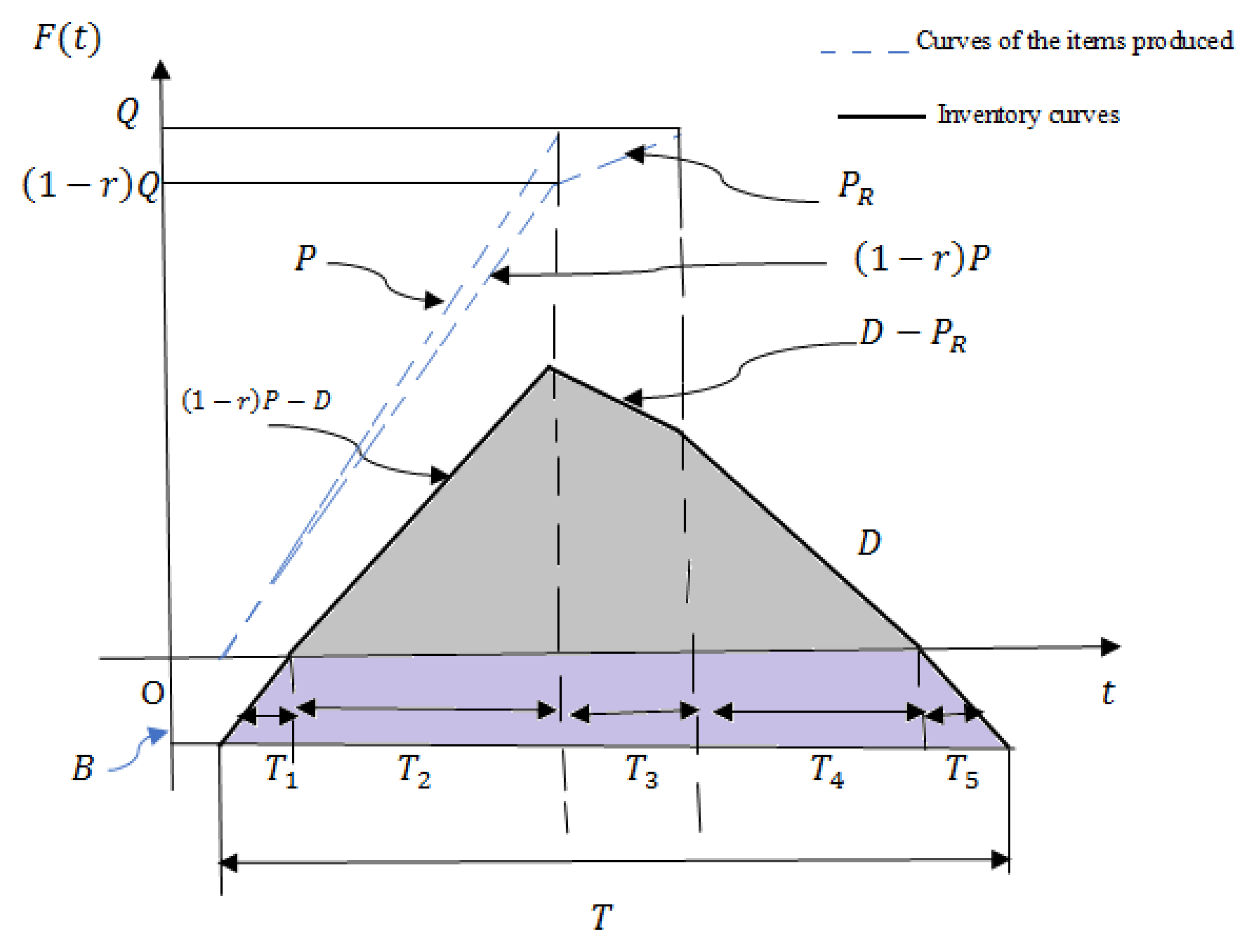
3.2. The P_R Is Lower than $D(P_R<D)$

If $P_R<D$, excellent items are retrieved from inventory at a faster rate than purchasing, resulting in a drop in inventory during the rework phase and a negative slope on the inventory curve. The inventory curves in this situation are depicted in Figure 5. The inventory curves for flawed products retain the same shape as in Figure 4.

The total inventory and backorder for the perfect items in the period $T_1$, $T_2$, $T_4$, $T_5$ and the inventory of flawed items for the period $T_3$ defined in Section 3.1 $(P_R>D)$ are the same in the case that $P_R<D$ as any assumption regarding $P_R$ has no effect on these values.

The inventory rate is decreasing during $T_3$, so the inventory curve during $T_3$ altered by $F_2\left(t\right)=\left(D-P_R\right)t+D{T}_4=\left(D-P_R\right)t+D\left(\frac{Q}{D}-\frac{B}{D}-\frac{Q}{P}-\frac{rQ}{P_R}\right)$ with the initial values $F_3\left(0\right)=F_3\left(T_4\right)=D\left(\frac{Q}{D}-\frac{B}{D}-\frac{Q}{P}-\frac{rQ}{P_R}\right)$.

Since $T_3=\frac{rQ}{P_R}$, the total inventory of perfect items during $T_3$ is ${{\displaystyle \int }}_0^{T_3}{F}_2\left(t\right)dt=\frac{1}{2}\left(D-P_R\right){\left(\frac{rQ}{P_R}\right)}^2+D\left(\frac{Q}{D}-\frac{B}{D}-\frac{Q}{P}-\frac{rQ}{P_R}\right)\left(\frac{rQ}{P_R}\right)$.

Hence, the average total cost per cycle and CO₂ for this case $P_R<D$ is

$$\begin{array}{cc}\hfill T{C}_{A2}\left(Q, S,B\right)& =\frac{SD}{Q}+\left(C_m+C_{R}r\right)D+b\left[\frac{1}{2}\frac{B^{2}D}{\left[\left(1-r\right)P-D\right]Q}+\frac{1}{2}\frac{B^2}{Q}\right]+\frac{C_{b}BD}{Q}\hfill \\ & +h_1\left[\frac{D}{Q}{\mathsf{\Pi }}_0\left(Q,B\right)+\frac{1}{2}\left(D-P_R\right)\left(\frac{r^{2}DQ}{P_R^2}\right)+{\mathsf{\Pi }}_5\left(Q,B\right)+{\mathsf{\Pi }}_2\left(Q,B\right)\right]\hfill \\ & +h_{2}DQ\left(\frac{1}{2}\frac{r}{P}+\frac{1}{2}\frac{r^2}{P_R}\right)+\tau Mln\left(\frac{S_0}{S}\right)\hfill \\ \mathrm{Subject} \mathrm{to} 0<S\le S_0\hfill & \end{array}$$

and

$$\begin{array}{cc}C{E}_{A2}\left(Q,B\right)=\frac{e_{s}D}{Q}& +D{e}_P+\frac{D}{Q}{e}_{T}d\hfill \\ & +e_{h1}\left[\frac{D}{Q}{\mathsf{\Pi }}_0\left(Q,B\right)+\frac{1}{2}\left(D-P_R\right)\left(\frac{r^{2}DQ}{P_R^2}\right)+{\mathsf{\Pi }}_5\left(Q,B\right)+{\mathsf{\Pi }}_2\left(Q,B\right)\right]\hfill \\ & +e_{h2}DQ\left(\frac{1}{2}\frac{r}{P}+\frac{1}{2}\frac{r^2}{P_R}\right)\hfill \end{array}$$

respectively.

Where ${\mathsf{\Pi }}_5\left(Q,B\right)=D^2\left(\frac{Q}{D}-\frac{B}{D}-\frac{Q}{P}-\frac{rQ}{P_R}\right)\left(\frac{r}{P_R}\right)$.

3.2.1. Carbon Tax with Quadratic Form of Green Investment

The average total cost when $P_R<D$ and quadratic form of investment for the present scenario is

$$\begin{gathered} \begin{array}{cc}\hfill T{C}_{Aq2}\left(Q, B, S,G\right)& =\left(S+{\mathsf{\Pi }}_3\left(B\right)\right)\frac{D}{Q}+\left(C_m+C_{R}r+C_t{e}_P{R}_1\left(G\right)\right)D+b\left[\frac{1}{2}\frac{B^{2}D}{\left[\left(1-r\right)P-D\right]Q}+\frac{1}{2}\frac{B^2}{Q}\right]\hfill \\ & +\left(C_t{e}_{h1}{R}_1\left(G\right)+h_1\right)\left[\frac{D}{Q}{\mathsf{\Pi }}_0\left(Q,B\right)+\frac{1}{2}\left(D-P_R\right)\left(\frac{r^{2}DQ}{P_R^2}\right)+{\mathsf{\Pi }}_5\left(Q,B\right)+{\mathsf{\Pi }}_2\left(Q,B\right)\right]\hfill \\ & +\left(C_t{e}_{h2}{R}_1\left(G\right)+h_2\right)DQ\left[\frac{1}{2}\frac{r}{P}+\frac{1}{2}\frac{r^2}{P_R}\right]+G-C_t{R}_1\left(G\right)+\tau Mln\left(\frac{S_0}{S}\right)\hfill \end{array} \\ \mathrm{Subject} \mathrm{to} 0<S\le S_0. \end{gathered}$$

(11)

Theorem 5.

For fixed$B,S and G$,$T{C}_{Aq2}\left(Q, B, S,G\right)$is convex in Q.

Proof. 

See Appendix E. □

Result 8.

By equating Equation (A5) to zero, the optimal$Q_{Aq2}$as

$$Q_{Aq2}^{*}={\left\{\frac{2\left(S+{\mathsf{\Pi }}_3\left(B\right)+\left(b+C_t{e}_{h1}{R}_1\left(G\right)+h_1\right)\frac{B^2}{2 }{\mathsf{\Pi }}_4\right)}{\left(C_t{e}_{h1}{R}_1\left(G\right)+h_1\right){∆}_2+\left(C_t{e}_{h2}{R}_1\left(G\right)+h_2\right)r\left[\frac{1}{P}+\frac{r}{P_R}\right]}\right\}}^{\frac{1}{2}}$$

(12)

Remark 2.

Equations (3)–(5) are still applicable to obtain the optimal$B_{Aq2}, S_{Aq2 }and G_{Aq2}$, respectively, under the case$P_R<D$since any assumption regarding$P_R$has no effect on these values. Moreover, we may utilize the same Algorithm 1 approach that was generated in the earlier part to obtain the optimal values in the present scenario.

3.2.2. Carbon Tax with Exponential form of Green Investment function

The total cost of the current scenario when $P_R<D$ per cycle is

$$\begin{array}{cc}\hfill T{C}_{AE2}\left(Q,B,G,S\right)& =\left(S+C_{b}B\right)\frac{D}{Q}+\left(C_m+C_{R}r\right)D+b\left[\frac{1}{2}\frac{B^{2}D}{\left[\left(1-r\right)P-D\right]Q}+\frac{1}{2}\frac{B^2}{Q}\right]\hfill \\ & +h_1\left[\frac{D}{Q}{\mathsf{\Pi }}_0\left(Q,B\right)+\frac{1}{2}\left(D-P_R\right)\left(\frac{r^{2}DQ}{P_R^2}\right)+{\mathsf{\Pi }}_5\left(Q,B\right)+{\mathsf{\Pi }}_2\left(Q,B\right)\right]\hfill \\ & +h_{2}DQ\left[\frac{1}{2}\frac{r}{P}+\frac{1}{2}\frac{r^2}{P_R}\right]+G-\left[C_{t}Z-C_{t}C{E}_{A2}\left\{1-\xi \left(1-e^{-mG}\right)\right\}\right]+\tau Mln\left(\frac{S_0}{S}\right)\hfill \\ & \mathrm{Subject} \mathrm{to} 0<S\le S_0.\hfill \end{array}$$

That is,

$$\begin{array}{cc}\hfill T{C}_{AE2}\left(Q,B,G,S\right)& =\left(S+{\tilde{\mathsf{\Pi }}}_3\left(B\right)\right)\frac{D}{Q}+\left(C_m+C_{R}r+C_t{e}_P\phi \right)D\hfill \\ & +\left(C_t{e}_{h1}\phi +h_1\right)\left[\frac{D}{Q}{\mathsf{\Pi }}_0\left(Q,B\right)+\frac{1}{2}\left(D-P_R\right)\left(\frac{r^{2}QD}{P_R^2}\right)+{\mathsf{\Pi }}_5\left(Q,B\right)+{\mathsf{\Pi }}_2\left(Q,B\right)\right]\hfill \\ & +b\left[\frac{1}{2}\frac{B^{2}D}{\left[\left(1-r\right)P-D\right]Q}+\frac{1}{2}\frac{B^2}{Q}\right]+\left(C_t{e}_{h2}\phi +h_2\right)QD\left[\frac{1}{2}\frac{r}{P}+\frac{1}{2}\frac{r^2}{P_R}\right]+G-C_{t}Z+\tau Mln\left(\frac{S_0}{S}\right)\hfill \\ & \mathrm{Subject} \mathrm{to} 0<S\le S_0\hfill \end{array}$$

(13)

The solution approach for problem (13) is similar to that of previous case Section 3.2.1. The same solution procedures are omitted in this theoretical derivation to avoid redundancy.

Result 9.

The optimal$Q_{AE2}$as

$$Q_{AE2}^{*}={\left\{\frac{2\left(S+{\tilde{\mathsf{\Pi }}}_3\left(B\right)+\left(b+C_t{e}_{h1}\phi +h_1\right)\frac{B^2}{2 }{\mathsf{\Pi }}_4\right)}{\left(C_t{e}_{h1}\phi +h_1\right){∆}_2+\left(C_t{e}_{h2}\phi +h_2\right)r\left[\frac{1}{P}+\frac{r}{P_R}\right]}\right\}}^{\frac{1}{2}}$$

(14)

Result 10.

The optimal$G_{AE2}$as

$$G_{AE2}^{*}=\frac{1}{m}\ln (C_{t}C{E}_{A2}\xi m)$$

(15)

Remark 3.

Equations (4) and (10) are still applicable to determine the optimal values of$B_{AE2} and S_{AE2}$, respectively, under the case$P_R<D$since any assumption regarding$P_R$has no effect on these values. Moreover, in the current scenario, we may utilize the same Algorithm 2 method that was generated in the preceding case to find the optimal values.

4. Production Scheduling with Synchronous Rework

The concept of a manufacturing process with synchronous rework offers the advantage of permitting faulty inventory items to be removed and backorders to be filled more quickly. There are two cases that must be investigated, and they are as follows: $P_R>D$ and $P_R<D$.

4.1. The $P_R$ Is Higher than D $\left(P_R>D\right)$

Figure 6 depicts the inventory curve of perfect items under the premise of synchronous rework, whereas Figure 7 depicts the inventory curve of flawed items.

The inventory curve has a slope ($\left(1-r\right)P+P_R-D)$ throughout the production period $T_1+T_2,$ since perfect items emerge from the rework process at a rate of $P_R$. Additionally, it is assumed that $P_R<rP$ to prevent disruption in the rework process.

During $T_1=\frac{B}{\left(1-r\right)P+P_R-D}$, the total amount of backorder is $\frac{B^2}{2\left[\left(1-r\right)P+P_R-D\right]}$. For the period $T_2=\frac{Q}{P}-\frac{B}{\left(1-r\right)P+P_R-D}$, the total amount of inventory ${\mathsf{\Pi }}_6\left(Q,B\right)=\frac{1}{2}\left(\left(1-r\right)P+P_R-D\right){\left(\frac{Q}{P}-\frac{B}{\left(1-r\right)P+P_R-D}\right)}^2$.

During $T_3=\frac{rQ}{P_R}-\frac{Q}{P}$, the amount of inventory is $\frac{1}{2}\left(P_R-D\right){\left(\frac{rQ}{P_R}-\frac{Q}{P}\right)}^2+\left(\left(1-r\right)P+P_R-D\right)\left(\frac{Q}{P}-\frac{B}{\left(1-r\right)P+P_R-D}\right)\left(\frac{rQ}{P_R}-\frac{Q}{P}\right)$. During $T_4=\frac{Q}{D}-\frac{B}{D}-\frac{rQ}{P_R}$, the total amount of inventory is $\frac{1}{2}D{\left(\frac{Q}{D}-\frac{B}{D}-\frac{rQ}{P_R}\right)}^2$. During $T_5=\frac{B}{D}$, the total backorder is $\frac{1}{2}\frac{B^2}{D}$.

The total inventory of flawed items may be calculated as follows: For time $T_1+T_2$, the total inventory of flawed items is $\frac{1}{2}\frac{rP-P_R}{P^2}{Q}^2$.

During $T_3$, the total inventory of flawed items is $\frac{1}{2}\frac{{\left(rP-P_R\right)}^2}{P_R{P}^2}{Q}^2$.

Then the average total cost per cycle for thecurrent case when $P_R>D$ is

$$\begin{array}{cc}\hfill T{C}_{\mathrm{S}1}\left(Q, B,S\right)=& \frac{SD}{Q}+\left(C_m+C_{R}r\right)D+b\left[\frac{B^{2}D}{2\left[\left(1-r\right)P+P_R-D\right]Q}+\frac{1}{2}\frac{B^2}{Q}\right]+\frac{C_{b}BD}{Q}\hfill \\ & +h_1\left[\frac{D}{2Q}{\mathsf{\Pi }}_6\left(Q,B\right)+{\mathsf{\Pi }}_8\left(Q\right)+{\mathsf{\Pi }}_6\left(Q,B\right)D\left(\frac{r}{P_R}-\frac{1}{P}\right)+{\mathsf{\Pi }}_7\left(Q,B\right)\right]\hfill \\ & +h_2\frac{DQ\left(rP-P_R\right)}{2P^2}\left[1+\frac{\left(rP-P_R\right)}{P_R}\right]+\tau Mln\left(\frac{S_0}{S}\right)\hfill \\ \mathrm{Subject} \mathrm{to} 0<S\le S_0\hfill & \end{array}$$

where ${\mathsf{\Pi }}_7\left(Q,B\right)=\frac{1}{2}\frac{D^2}{Q}{\left(\frac{Q}{D}-\frac{B}{D}-\frac{rQ}{P_R}\right)}^2$ and ${\mathsf{\Pi }}_8\left(Q\right)=\frac{1}{2}\left(P_R-D\right)DQ{\left(\frac{r}{P_R}-\frac{1}{P}\right)}^2$.

Then, the CO₂ is given by

$$\begin{array}{cc}\hfill C{E}_{\mathrm{S}1}\left(Q,B\right)=\frac{e_{s}D}{Q}& +D{e}_P+\frac{D}{Q}{e}_{T}d+e_{h2}\frac{DQ}{2P^2}\left[\left(rP-P_R\right)+\frac{{\left(rP-P_R\right)}^2}{P_R}\right]\hfill \\ & +e_{h1}\left[\frac{D}{2Q}{\mathsf{\Pi }}_6\left(Q,B\right)+{\mathsf{\Pi }}_8\left(Q\right)+{\mathsf{\Pi }}_6\left(Q,B\right)\left(\frac{r}{P_R}-\frac{1}{P}\right)D+{\mathsf{\Pi }}_7\left(Q,B\right)\right]\hfill \end{array}$$

4.1.1. Carbon Tax with Quadratic form of Green Investment Function

The average total cost per cycle with variable green investment is

$$\begin{gathered} \begin{array}{cc}\hfill T{C}_{Sq1}\left(Q, B,S,G\right)& =\left(S+{\mathsf{\Pi }}_3(B\right)\frac{D}{Q}+\left(C_m+C_{R}r+C_t{e}_P{R}_1\left(G\right)\right)D\hfill \\ & +b\left[\frac{B^{2}D}{2\left[\left(1-r\right)P+P_R-D\right]Q}+\frac{1}{2}\frac{B^2}{Q}\right]\hfill \end{array} \\ \begin{array}{c}+\left(C_t{e}_{h1}{R}_1\left(G\right)+h_1\right)\left[\frac{D}{2Q}{\mathsf{\Pi }}_6\left(Q,B\right)+{\mathsf{\Pi }}_8\left(Q\right)+{\mathsf{\Pi }}_6\left(Q,B\right)\left(\frac{r}{P_R}-\frac{1}{P}\right)D+{\mathsf{\Pi }}_7\left(Q,B\right)\right]\hfill \\ +\left(C_t{e}_{h2}{R}_1\left(G\right)+h_2\right)\frac{DQ}{2P^2}\left[\left(rP-P_R\right)+\frac{{\left(rP-P_R\right)}^2}{P_R}\right]\hfill \\ +G-C_t\left[Z-C{E}_{\mathrm{S}1}\left(Q,B\right)R_1\left(G\right)\right]+\tau Mln\left(\frac{S_0}{S}\right)\hfill \\ \mathrm{Subject} \mathrm{to} 0<S\le S_0.\hfill \end{array} \end{gathered}$$

(16)

Theorem 6.

For fixed$B,S and G$,$T{C}_{Sq1}\left(Q, B,S,G\right)$is convex in Q.

Proof. 

See Appendix F. □

Result 11.

By equating Equation (A6) to zero, the optimal$Q_{Sq1}$as

$$Q_{Sq1}^{*}={\left\{\frac{2\left(S+{\mathsf{\Pi }}_3\left(B\right)+\left(b+C_t{e}_{h1}{R}_1\left(G\right)+h_1\right)\frac{B^2}{2 }{\mathsf{\Pi }}_9\right)}{\left(C_t{e}_{h1}{R}_1\left(G\right)+h_1\right){∆}_3+\left(C_t{e}_{h2}{R}_1\left(G\right)+h_2\right)\frac{\left(rP-P_R\right)}{P^2}\left[1+\frac{\left(rP-P_R\right)}{P_R}\right]}\right\}}^{\frac{1}{2}}$$

(17)

Theorem 7.

For fixed$Q,S and G$,$T{C}_{Sq1}\left(Q, B,S,G\right)$is convex in B.

Proof. 

See Appendix G. □

Result 12.

By equating Equation (A7) to zero, the optimal$B_{Sq1}$as

$$B_{Sq1}^{*}=\frac{Q\left(C_t{e}_{h1}{R}_1\left(G\right)+h_1\right)-D{C}_b}{\left[\frac{D}{\left(\left(1-r\right)P+P_R-D\right)}+1\right]\left(b+C_t{e}_{h1}{R}_1\left(G\right)+h_1\right)}$$

(18)

Remark 4.

Equations (4) and (5) are still applicable to obtain the optimal$S_{Sq1} and G_{Sq1}$, respectively, under the case of quadratic green investment since any assumption regarding synchronous rework has no effect on these values. Moreover, we can utilize the same Algorithm 1 from Section 3 to obtain the optimal values for the current situation.

4.1.2. Carbon Tax with Exponential form of Green Investment Function

With exponential green investment, the average total cost per cycle is

$$\begin{array}{cc}\hfill T{C}_{SE1}\left(Q, B,S,G\right)& =\left(S+C_{b}B\right)\frac{D}{Q}+\left(C_m+C_{R}r\right)D+b\left[\frac{B^{2}D}{2\left[\left(1-r\right)P+P_R-D\right]Q}+\frac{1}{2}\frac{B^2}{Q}\right]\hfill \\ & +h_1\left[\frac{D}{2Q}{\mathsf{\Pi }}_6\left(Q,B\right)+{\mathsf{\Pi }}_6\left(Q,B\right)\left(\frac{r}{P_R}-\frac{1}{P}\right)D+{\mathsf{\Pi }}_8\left(Q\right)+{ \mathsf{\Pi }}_7\left(Q,B\right)\right]\hfill \\ & +\tau Mln\left(\frac{S_0}{S}\right)+h_2\frac{DQ}{2P^2}\left[\left(rP-P_R\right)+\frac{{\left(rP-P_R\right)}^2}{P_R}\right]+G-C_t\left[Z-C_{t}C{E}_7\left(1-\xi \left(1-e^{-mG}\right)\right)\right]\hfill \\ & \mathrm{Subject} \mathrm{to} 0<S\le S_0.\hfill \end{array}$$

That is,

$$\begin{array}{cc}\hfill T{C}_{SE1}\left(Q, B,S,G\right)& =\left(S+{\tilde{\mathsf{\Pi }}}_3\left(B\right)\right)\frac{D}{Q}+\left(C_m+C_{R}r+C_t{e}_P\phi \right)D+b\left[\frac{1}{2}\frac{B^{2}D}{\left[\left(1-r\right)P+P_R-D\right]Q}+\frac{1}{2}\frac{B^2}{Q}\right]\hfill \\ & +\left(C_t{e}_{h1}\phi +h_1\right)\left[\frac{D}{2Q}{\mathsf{\Pi }}_6\left(Q,B\right)+{ \mathsf{\Pi }}_8\left(Q\right)+{\mathsf{\Pi }}_6\left(Q,B\right)\left(\frac{r}{P_R}-\frac{1}{P}\right)D+{\mathsf{\Pi }}_7\left(Q,B\right)\right]\hfill \\ & +\left(C_t{e}_{h2}\phi +h_2\right)\frac{DQ}{2P^2}\left[\left(rP-P_R\right)+\frac{{\left(rP-P_R\right)}^2}{P_R}\right]+G-C_{t}Z+\tau Mln\left(\frac{S_0}{S}\right)\hfill \\ & \mathrm{Subject} \mathrm{to} 0<S\le S_0.\hfill \end{array}$$

(19)

The solution approach for Problem (19) is similar to that of previous case Section 4.1.1. The same solution procedures are omitted in this theoretical derivation to avoid redundancy.

Result 13.

The optimal$Q_{SE1}$as

$$Q_{SE1}^{*}={\left\{\frac{2\left[S+{\tilde{\mathsf{\Pi }}}_3\left(B\right)+\left(b+C_t{e}_{h1}\phi +h_1\right)\frac{B^2}{2 }{\mathsf{\Pi }}_9\right]}{\left(C_t{e}_{h1}\phi +h_1\right){∆}_3+\left(C_t{e}_{h2}\phi +h_2\right)\frac{\left(rP-P_R\right)}{P^2}\left[1+\frac{\left(rP-P_R\right)}{P_R}\right]}\right\}}^{\frac{1}{2}}$$

(20)

Result 14.

The optimal$B_{SE1}$as

$$B_{SE1}^{*}=\frac{Q\left(C_t{e}_{h1}\phi +h_1\right)-D{C}_b}{\left[\frac{D}{\left(\left(1-r\right)P+P_R-D\right)}+1\right]\left(b+C_t{e}_{h1}\phi +h_1\right)}$$

(21)

Result 15.

The optimal$G_{SE1}$as

$$G_{SE1}^{*}=\frac{1}{m}\ln (C_t C{E}_{S1}\xi m).$$

(22)

Remark 5.

Equation (4) is still valid to determine the optimal$S_{SE1}$under the exponential green investment case since this value does not change by any assumption about synchronous rework. Furthermore, we may use Algorithm 1 from Section 3 to obtain the optimal values for the current scenario.

4.2. The $P_R$ Is Lower than D $\left(P_R<D\right)$

Figure 8 depicts the inventory curve for perfect items. When $P_R>D$, as shown in Figure 7, the inventory curves of flawed items have the same functional forms as flawed items. The inventory curve of the perfect products during $T_3$ is $F_2\left(t\right)=\left(D-P_R\right)t+D\left(\frac{Q}{D}-\frac{B}{D}-\frac{rQ}{P_R}\right)$ with the initial value $F_2\left(0\right)=D\left(\frac{Q}{D}-\frac{B}{D}-\frac{rQ}{P_R}\right)$.

During $T_3=\frac{rQ}{P_R}-\frac{Q}{P}$, the total inventory is

$${{\displaystyle \int }}_0^{T_3}{F}_2\left(t\right)dt=\frac{1}{2}\left(D-P_R\right){\left(\frac{rQ}{P_R}-\frac{Q}{P}\right)}^2+D\left(\frac{Q}{D}-\frac{B}{D}-\frac{rQ}{P_R}\right)\left(\frac{rQ}{P_R}-\frac{Q}{P}\right).$$

Inventory cost per cycle for the current scenario when $P_R<D$ is

$$\begin{array}{cc}\hfill T{C}_{S2}\left(Q,B,G\right)& =\left(S+C_{b}B\right)\frac{D}{Q}+\left(C_m+C_{R}r\right)D+b\left[\frac{B^{2}D}{2\left[\left(1-r\right)P+P_R-D\right]Q}+\frac{1}{2}\frac{B^2}{Q}\right]\hfill \\ & +h_1[\frac{1}{2}\frac{\left(\left(1-r\right)P+P_R-D\right)D}{Q}{\left(\frac{Q}{P}-\frac{B}{\left(1-r\right)P+P_R-D}\right)}^2+{\mathsf{\Pi }}_{11}\left(Q\right)\hfill \\ & +D^2\left(\frac{Q}{D}-\frac{B}{D}-\frac{rQ}{P_R}\right)\left(\frac{r}{P_R}-\frac{1}{P}\right)+{\mathsf{\Pi }}_7\left(Q,B\right)]+\frac{DQ{h}_2}{2P^2}\left(rP-P_R\right)\left[1+\frac{\left(rP-P_R\right)}{P_R}\right]+\tau Mln\left(\frac{S_0}{S}\right)\hfill \\ & \mathrm{Subject} \mathrm{to} 0<S\le S_0.\hfill \end{array}$$

where ${\mathsf{\Pi }}_{11}\left(Q\right)=\frac{1}{2}DQ\left(D-P_R\right){\left(\frac{r}{P_R}-\frac{1}{P}\right)}^2$.

Then the CO₂ is given by

$$\begin{array}{cc}\hfill C{E}_{S2}\left(Q,B\right)=\frac{e_{s}D}{Q}& +D{e}_P+\frac{D}{Q}{e}_{T}d\hfill \\ & +e_{h1}\left[\frac{D}{2Q}{\mathsf{\Pi }}_6\left(Q,B\right)+{\mathsf{\Pi }}_{11}\left(Q\right)+D^2\left(\frac{Q}{D}-\frac{B}{D}-\frac{rQ}{P_R}\right)\left(\frac{r}{P_R}-\frac{1}{P}\right)+{\mathsf{\Pi }}_7\left(Q,B\right)\right]\hfill \\ & +e_{h2}\frac{DQ}{2P^2}\left(rP-P_R\right)\left[1+\frac{\left(rP-P_R\right)}{P_R}\right]\hfill \end{array}$$

4.2.1. Carbon Tax with Quadratic form of Green Investment Function

The average total cost when $P_R<D$ with the quadratic form of investment is

$$\begin{array}{cc}\hfill T{C}_{Sq2}\left(Q, B, S,G\right)& =\left(S+{\mathsf{\Pi }}_3\left(B\right)\right)\frac{D}{Q}+\left(C_m+C_{R}r+C_t{e}_P{R}_1\left(G\right)\right)D\hfill \\ & +b\left[\frac{B^{2}D}{2\left[\left(1-r\right)P+P_R-D\right]Q}+\frac{1}{2}\frac{B^2}{Q}\right]\hfill \\ & +\left(C_t{e}_{h1}{R}_1\left(G\right)+h_1\right)[\frac{D}{2Q}{\mathsf{\Pi }}_6\left(Q,B\right)+{\mathsf{\Pi }}_{11}\left(Q\right)+D^2\left(\frac{Q}{D}-\frac{B}{D}-\frac{rQ}{P_R}\right)\left(\frac{r}{P_R}-\frac{1}{P}\right)\hfill \\ & +{\mathsf{\Pi }}_7\left(Q,B\right)]+\left(C_t{e}_{h2}{R}_1\left(G\right)+h_2\right)\frac{DQ}{2P^2}\left(rP-P_R\right)\left[1+\frac{\left(rP-P_R\right)}{P_R}\right]+G\hfill \\ & -C_t\left[Z-C{E}_{S2}\left(Q,B\right)R_1\left(G\right)\right]+\tau Mln\left(\frac{S_0}{S}\right)\hfill \\ & \mathrm{Subject} \mathrm{to} 0<S\le S_0.\hfill \end{array}$$

(23)

Theorem 8.

For fixed$B,S and G$,$T{C}_{Sq2 }\left(Q,B, S,G\right)$is convex in Q.

Proof. 

See Appendix H. □

Result 16.

By setting Equation (A8) to zero, the optimal$Q_{Sq2}$as

$$Q_{Sq2}^{*}={\left\{\frac{2\left(S+{\mathsf{\Pi }}_3\left(B\right)+\left(b+C_t{e}_{h1}{R}_1\left(G\right)+h_1\right)\frac{B^2}{2 }{\mathsf{\Pi }}_9\right)}{\left(C_t{e}_{h1}{R}_1\left(G\right)+h_1\right){∆}_4+\left(C_t{e}_{h2}{R}_1\left(G\right)+h_2\right)\frac{\left(rP-P_R\right)}{P^2}\left[1+\frac{\left(rP-P_R\right)}{P_R}\right]}\right\}}^{\frac{1}{2}}$$

(24)

Remark 6.

Equations (4), (5) and (18) are still applicable to determine the optimal values of$B_{Sq2}, S_{Sq2} and G_{Sq2}$, respectively, under the case$P_R<D$since any assumption regarding$P_R$has no effect on these values. Moreover, in the present scenario, we may utilize the same Algorithm 1 method that was generated in the preceding case to find the optimal values.

4.2.2. Carbon Tax with Exponential form of Green Investment Function

The average total cost with exponential green investment is

$$\begin{array}{cc}T{C}_{SE2}\left(Q, B,S,G\right)\hfill & =S\frac{D}{Q}+\left(C_m+C_{R}r\right)D+b\left[\frac{1}{2}\frac{B^{2}D}{\left[\left(1-r\right)P+P_R-D\right]Q}+\frac{1}{2}\frac{B^2}{Q}\right]\hfill \\ & +h_1\left[\frac{D}{2Q}{\mathsf{\Pi }}_6\left(Q,B\right)+{\mathsf{\Pi }}_{11}\left(Q\right)+D^2\left(\frac{Q}{D}-\frac{B}{D}-\frac{rQ}{P_R}\right)\left(\frac{r}{P_R}-\frac{1}{P}\right)+{\mathsf{\Pi }}_7\left(Q,B\right)\right]\hfill \\ & +\left(C_t{e}_{h2}+h_2\right)\frac{DQ}{2P^2}\left(rP-P_R\right)\left[1+\frac{\left(rP-P_R\right)}{P_R}\right]+G\hfill \\ & -C_t\left[Z-C{E}_{S2} \left(1-\xi \left(1-e^{-mG}\right)\right)\right]+\tau Mln\left(\frac{S_0}{S}\right)\hfill \\ & \mathrm{Subject} \mathrm{to} 0<S\le S_0. \hfill \end{array}$$

That is,

$$\begin{array}{cc}T{C}_{SE2}\left(Q, B, S,G\right)\hfill & =\left(S+{\tilde{\mathsf{\Pi }}}_3\left(B\right)\right)\frac{D}{Q}+\left(C_m+C_{R}r+C_t{e}_P\phi \right)+\frac{b{B}^{2}D}{2Q}\left[\frac{1}{\left[\left(1-r\right)P+P_R-D\right]Q}+\frac{1}{D}\right]\hfill \\ & +\left(C_t{e}_{h1}\phi +h_1\right)\left[\frac{D}{2Q}{\mathsf{\Pi }}_6\left(Q,B\right)+{\mathsf{\Pi }}_{11}\left(Q\right)+D^2\left(\frac{Q}{D}-\frac{B}{D}-\frac{rQ}{P_R}\right)\left(\frac{r}{P_R}-\frac{1}{P}\right)+{\mathsf{\Pi }}_7\left(Q,B\right)\right]\hfill \\ & +\left(C_t{e}_{h2}\phi +h_2\right)\frac{DQ}{2P^2}\left[\left(rP-P_R\right)+\frac{{\left(rP-P_R\right)}^2}{P_R}\right]+G-C_{t}Z+\tau Mln\left(\frac{S_0}{S}\right)\hfill \\ & \mathrm{Subject} \mathrm{to} 0<S\le S_0.\hfill \end{array}$$

(25)

The solution approach for problem (25) is similar to that of previous case Section 4.2.1. The same solution procedures are omitted in this theoretical derivation to avoid redundancy.

Result 17.

The optimal$Q_{SE2}$as

$$Q_{SE2}^{*}={\left\{\frac{2\left(S+{\tilde{\mathsf{\Pi }}}_3\left(B\right)+\left(b+C_t{e}_{h1}\phi +h_1\right)\frac{B^2}{2 }{\mathsf{\Pi }}_9\right)}{\left(C_t{e}_{h1}\phi +h_1\right){∆}_4+\left(C_t{e}_{h2}\phi +h_2\right)\frac{\left(rP-P_R\right)}{P^2}\left[1+\frac{\left(rP-P_R\right)}{P_R}\right]}\right\}}^{\frac{1}{2}}$$

Result 18.

The optimal$G_{SE2 }$as

$$G_{SE2}^{*}=\frac{1}{m}\ln (C_{t}C{E}_{S2}\xi m).$$

Remark 7.

Equations (4) and (21) are still valid to obtain the optimal$B_{SE2}$and$S_{SE2}$, respectively, under the case$P_R<D$since any assumption regarding$P_R$has no effect on these values. Furthermore, we may utilize the same Algorithm 2 approach that was generated in the preceding case to obtain the optimal values in the present scenario.

5. Numerical and Sensitivity Assessment

5.1. Asynchronous Rework

We will utilize numerical assessment to explain the solution approach in this section. The subsequent parameters have values that are very close to those in Al-Salamah [17] and Mishra [33]: D = 4800 units, P = 24,000 units/year, $S_0$ = $120, $C_m=\$3.1,$ r = 0.01, $h_1$ = $0.6/unit/year, $h_2$ = 0.3/unit/year, $C_b$= $0.1/unit short, b = $14.4/unit short/year, $C_R$ = $0.000125$P_R$/unit, Z = 900 kg/year, $C_t=0.33 \mathrm{kg}/\mathrm{year} ,m=0.8$ unit, $\xi =0.2$ unit, $e_P=40 \mathrm{kg}/\mathrm{year}$, $e_s=60 \mathrm{kg}/\mathrm{year}, e_{h1}=4 \mathrm{kg}/\mathrm{year}, e_{h2}=3 \mathrm{kg}/\mathrm{year}, e_T=50 \mathrm{kg}/\mathrm{year}, d=100,000 \mathrm{kg}/\mathrm{year}$, $\tau =0.1/\mathrm{year}, M=5800.$

We study the variations in optimal solutions subject to two main parameters r and $P_R$ for both quadratic and exponential cases. All the parameters are retained constant in the initial event, with the exclusion of r, which is altered to see how it affects decision variables for both quadratic ($Q_{Aqi}$, $B_{Aqi}$,$G_{Aqi},S_{Aqi}$) and exponential $(Q_{AEi}$, $B_{AEi}$,$G_{AEi},S_{AEi}$) cases, $i=1,2$. Similarly, the rework rate $P_R$ is examined in the second event to see how the values of decision variables for both cases vary for low and high rework rates.

Table 2. Changeable r and asynchronous rework with $P_R>D$.

Asynchronous Rework ${\mathit{P}}_{\mathit{R}}>\mathit{D}$
Quadratic Green Investment Function
	With Green Investment						Without Green Investment
r	${\mathit{Q}}_{\mathit{A}\mathit{q}1}$	${\mathit{B}}_{\mathit{A}\mathit{q}1}$	${\mathit{G}}_{\mathit{A}\mathit{q}1}$	${\mathit{S}}_{\mathit{A}\mathit{q}1}$	$\mathit{C}{\mathit{E}}_{\mathit{A}1}\left(.\right)$	$\mathit{T}{\mathit{C}}_{\mathit{A}\mathit{q}1}\left(.\right)$	${\mathit{Q}}_{\mathit{A}\mathit{q}1}$	${\mathit{B}}_{\mathit{A}\mathit{q}1}$	${\mathit{G}}_{\mathit{A}\mathit{q}1}$	${\mathit{S}}_{\mathit{A}\mathit{q}1}$	$\mathit{C}{\mathit{E}}_{\mathit{A}1}\left(.\right)$	$\mathit{T}{\mathit{C}}_{\mathit{A}\mathit{q}1}\left(.\right)$	Savings (%)
0.01	1343	21.6	160	75	602	309,276	1398	23.8	-	-	711	335,231	8.4
0.05	1352	20.4	171	81	625	317,634	1426	22.4	-	-	735	354,374	11.6
0.10	1361	19.1	182	85	641	324,569	1456	21.6	-	-	751	372,371	14.7
0.15	1369	18.9	196	87	650	331,548	1471	20.8	-	-	761	385,365	16.2
0.20	1378	18.1	202	92	676	339,876	1498	20.1	-	-	790	400,273	17.7
0.25	1386	17.6	216	94	693	347,984	1516	19.5	-	-	813	415,076	19.3
0.30	1392	16.7	231	100	721	356,654	1535	18.7	-	-	861	434,067	21.7
0.35	1410	15.1	253	102	748	362,098	1550	17.7	-	-	899	448,071	23.7
0.40	1423	14.7	271	104	774	384,876	1574	16.6	-	-	957	481,379	25.1
Exponential Green Investment Function
	With Green Investment						Without Green Investment
r	$Q_{AE1}$	$B_{AE1}$	$G_{AE1}$	$S_{AE1}$	$C{E}_{A1}\left(.\right)$	$T{C}_{AE1}\left(.\right)$	$Q_{AE1}$	$B_{AE1}$	$G_{AE1}$	$S_{AE1}$	$C{E}_{A1}\left(.\right)$	$T{C}_{AE1}\left(.\right)$	Savings (%)
0.01	1391	22.2	172	77	602	309,316	1391	22.4	-	-	711	336,132	8.6
0.05	1402	20.9	183	85	625	317,743	1402	21.3	-	-	735	354,794	11.7
0.10	1410	20.1	194	87	641	324,641	1410	20.8	-	-	751	372,729	14.8
0.15	1448	19.8	208	89	650	331,678	1448	20.5	-	-	761	386,481	16.5
0.20	1462	19.1	221	99	676	339,991	1462	20.1	-	-	790	401,104	17.9
0.25	1516	18.2	231	102	693	348,220	1516	19.5	-	-	813	417,026	19.7
0.30	1542	17.4	243	104	721	356,743	1542	18.1	-	-	861	436,071	22.2
0.35	1571	16.1	269	106	748	362,142	1571	17.6	-	-	899	448,631	23.8
0.40	1598	15.3	281	109	774	384,966	1598	17.1	-	-	957	483,003	25.5

reveals the optimal $Q_{Aq1}$, $B_{Aq1}$,$G_{Aq1}$ and $S_{Aq1}$ for a range of values of r when $P_R$ = 40,000 items/year. The result is compared to the total cost with and without the green investment, which is also included in Table 2, to show how reducing setup costs and CO₂ affect each other. Figure 9 and Figure 10 visualize the flctuations of CO₂ against r with and without green investment vs. r when $P_R>D.$

5.2. Synchronous Rework

We will utilize the same firm as in the preceding section, but this time we will assume that products with flaws are fixed as soon as they are made. Once the manufacturing lot is complete, each defective item that was not corrected during production is individually remade.The model must meet the assumptions that $P_R<rP$ and $D<P_R$, according to Al-Salamah [17], which states that D = 190 items per year and $P_R=200$ items per year. In

Table 3. Changeable r and synchronous rework with $P_R>D$.

Synchronous Rework ${\mathit{P}}_{\mathit{R}}>\mathit{D}$
Quadratic Green Investment Function
	With Green Investment						Without Green Investment
r	${\mathit{Q}}_{\mathit{S}\mathit{q}1}$	${\mathit{B}}_{\mathit{S}\mathit{q}1}$	${\mathit{G}}_{\mathit{S}\mathit{q}1}$	${\mathit{S}}_{\mathit{S}\mathit{q}1}$	$\mathit{C}{\mathit{E}}_{\mathit{S}1}\left(.\right)$	$\mathit{T}{\mathit{C}}_{\mathit{S}\mathit{q}1}\left(.\right)$	${\mathit{Q}}_{\mathit{S}\mathit{q}1}$	${\mathit{B}}_{\mathit{S}\mathit{q}1}$	${\mathit{G}}_{\mathit{S}\mathit{q}1}$	${\mathit{S}}_{\mathit{S}\mathit{q}1}$	$\mathit{C}{\mathit{E}}_{\mathit{S}1}\left(.\right)$	$\mathit{T}{\mathit{C}}_{\mathit{S}\mathit{q}1}\left(.\right)$	Savings (%)
0.01	1364	22.3	165	81	612	317,964	1432	24.6	-	-	732	349,941	10.1
0.05	1371	21.4	176	86	627	324,587	1464	23.5	-	-	753	365,248	12.5
0.10	1379	20.6	184	92	638	339,641	1494	22.7	-	-	778	385,742	13.6
0.15	1385	19.5	193	98	652	348,423	1531	21.2	-	-	791	401,345	15.2
0.20	1394	18.6	210	104	671	356,214	1549	20.1	-	-	820	418,476	17.5
0.25	1399	17.2	219	109	690	367,198	1563	19.5	-	-	847	436,546	18.9
0.30	1411	16.7	236	114	712	376,347	1585	18.3	-	-	876	451,253	19.9
0.35	1420	15.4	254	117	735	383,695	1598	17.6	-	-	910	470,197	22.6
0.40	1432	14.7	278	121	760	394,322	1627	16.4	-	-	968	488,752	24.0
Exponential green investment function
	With green investment						Without green investment
r	$Q_{SE1}$	$B_{SE1}$	$G_{SE1}$	$S_{SE1}$	$C{E}_{S1}\left(.\right)$	$T{C}_{SE1}\left(.\right)$	$Q_{SE1}$	$B_{SE1}$	$G_{SE1}$	$S_{SE1}$	$C{E}_{S1}\left(.\right)$	$T{C}_{SE1}\left(.\right)$	Savings (%)
0.01	1398	21.6	176	81	612	309,867	1442	24.9	-	-	732	342,954	10.7
0.05	1416	20.3	187	92	627	319,675	1456	22.8	-	-	753	361,056	13.0
0.10	1423	18.5	196	99	638	328,542	1479	20.5	-	-	778	380,864	15.9
0.15	1439	17.1	201	105	652	339,671	1493	19.3	-	-	791	402,217	18.4
0.20	1451	16.4	225	110	671	344,755	1513	18.2	-	-	820	411,245	19.3
0.25	1476	15.7	251	114	690	359,876	1532	17.8	-	-	847	430,976	19.8
0.30	1586	14.9	269	118	712	367,423	1580	16.9	-	-	876	443,547	20.7
0.35	1594	14.1	282	121	735	372,547	1612	16.4	-	-	910	454,245	21.9
0.40	1607	13.5	290	125	760	389,451	1635	16.1	-	-	968	486,547	24.9

, the results are compared to the total cost with and without the green investment. The visual comparison of CO₂ and tax with and without green investment vs. r when $P_R>D$ is shown in Figure 11 and Figure 12.

5.3. Discussion and Comparison of Findings

This study explores the connection between green investments and CO₂. Using the quadratic and exponential forms of CO₂ reduction functions offered by Huang et al. [32] and Mishra et al. [33], this study examines the dependence structure between green technology and CO₂.

• According to Table 2, Table 3,

  Table 4. Changeable r and asynchronous rework with $P_R<D$.

  $\mathbf{Asynchronous} \mathbf{Rework} {\mathit{P}}_{\mathit{R}}<\mathit{D}$
  Quadratic Green Investment Function
  	With Green Investment						Without Green Investment
  r	${\mathit{Q}}_{\mathit{A}\mathit{q}2}$	${\mathit{B}}_{\mathit{A}\mathit{q}2}$	${\mathit{G}}_{\mathit{A}\mathit{q}2}$	${\mathit{S}}_{\mathit{A}\mathit{q}2}$	$\mathit{C}{\mathit{E}}_{\mathit{A}2}\left(.\right)$	$\mathit{T}{\mathit{C}}_{\mathit{A}\mathit{q}2}\left(.\right)$	${\mathit{Q}}_{\mathit{A}\mathit{q}2}$	${\mathit{B}}_{\mathit{A}\mathit{q}2}$	${\mathit{G}}_{\mathit{A}\mathit{q}2}$	${\mathit{S}}_{\mathit{A}\mathit{q}2}$	$\mathit{C}{\mathit{E}}_{\mathit{A}2}\left(.\right)$	$\mathit{T}{\mathit{C}}_{\mathit{A}\mathit{q}2}\left(.\right)$	Savings (%)
  0.01	1659	22.3	171	82	611	311,564	1721	24.5	-	-	731	341,165	9.5
  0.05	1668	21.5	179	89	637	319,785	1739	23.6	-	-	755	357,874	11.9
  0.10	1679	19.1	186	95	651	330,219	1770	22.4	-	-	771	376,247	13.9
  0.15	1691	18.4	195	102	672	338,425	1782	21.7	-	-	786	390,014	15.2
  0.20	1705	17.5	214	109	689	342,100	1798	19.7	-	-	811	406,570	18.8
  0.25	1716	16.2	231	115	706	348,589	1817	18.5	-	-	829	418,214	20.0
  0.30	1723	15.1	245	119	750	360,210	1836	18.0	-	-	864	441,429	22.6
  0.35	1728	14.3	271	124	789	375,674	1860	17.4	-	-	932	465,478	23.9
  0.40	1739	13.8	292	134	814	396,574	1895	17.3	-	-	976	495,425	24.9
  Exponential green investment function
  	With green investment						Without green investment
  r	$Q_{AE2}$	$B_{AE2}$	$G_{AE2}$	$S_{AE2}$	$C{E}_{A2}\left(.\right)$	$T{C}_{AE2}\left(.\right)$	$Q_{AE2}$	$B_{AE2}$	$G_{AE2}$	$S_{AE2}$	$C{E}_{A2}\left(.\right)$	$T{C}_{AE2}\left(.\right)$	Savings (%)
  0.01	1668	22.6	181	86	611	312,458	1712	24.6	-	-	731	343,214	9.8
  0.05	1718	21.3	189	92	637	325,013	1741	23.6	-	-	755	358,478	10.3
  0.10	1730	20.4	211	98	651	342,480	1769	22.7	-	-	771	379,987	11.0
  0.15	1759	19.1	224	111	672	351,245	1784	21.8	-	-	786	397,163	13.1
  0.20	1831	18.3	230	116	689	359,654	1821	21.0	-	-	811	411,245	14.3
  0.25	1870	17.4	241	120	706	368,412	1830	19.3	-	-	829	425,741	15.6
  0.30	1892	15.8	263	125	750	375,147	1854	18.4	-	-	864	438,320	16.8
  0.35	1915	14.9	280	129	789	385,430	1876	17.3	-	-	932	462,147	19.9
  0.40	1956	14.1	291	134	814	396,478	1899	16.9	-	-	976	489,217	23.4

  and

  Table 5. Changeable r and synchronous rework with $P_R<D$.

  $\mathbf{Synchronous} \mathbf{Rework} {\mathit{P}}_{\mathit{R}}<\mathit{D}$
  Quadratic Green Investment Function
  	With Green Investment						Without Green Investment
  r	${\mathit{Q}}_{\mathit{S}\mathit{q}2}$	${\mathit{B}}_{\mathit{S}\mathit{q}2}$	${\mathit{G}}_{\mathit{S}\mathit{q}2}$	${\mathit{S}}_{\mathit{S}\mathit{q}2}$	$\mathit{C}{\mathit{E}}_{\mathit{S}\mathit{q}2}\left(.\right)$	$\mathit{T}{\mathit{C}}_{\mathit{S}\mathit{q}1}\left(.\right)$	${\mathit{Q}}_{\mathit{S}\mathit{q}2}$	${\mathit{B}}_{\mathit{S}\mathit{q}2}$	${\mathit{G}}_{\mathit{S}\mathit{q}2}$	${\mathit{S}}_{\mathit{S}\mathit{q}2}$	$\mathit{C}{\mathit{E}}_{\mathit{S}2}\left(.\right)$	$\mathit{T}{\mathit{C}}_{\mathit{S}\mathit{q}2}\left(.\right)$	Savings (%)
  0.01	1656	21.9	162	78	609	310,387	1715	24.1	-	-	723	340,124	9.5
  0.05	1663	20.7	173	84	632	319,978	1733	23.3	-	-	747	361,248	12.9
  0.10	1672	18.4	184	89	648	325,741	1762	22.5	-	-	768	375,687	15.3
  0.15	1680	17.6	198	94	659	336,425	1777	21.8	-	-	781	392,755	16.7
  0.20	1689	17.1	211	97	685	352,413	1794	19.9	-	-	804	415,547	17.9
  0.25	1698	16.2	225	101	692	361,214	1812	19.1	-	-	839	429,578	18.9
  0.30	1706	15.1	241	104	770	372,457	1832	18.4	-	-	871	445,874	19.7
  0.35	1718	14.5	264	107	786	385,424	1857	17.6	-	-	910	463,856	20.4
  0.40	1732	13.9	282	110	799	389,842	1883	17.1	-	-	964	476,254	22.2
  Exponential green investment function
  	With green investment						Without green investment
  r	$Q_{SE2}$	$B_{SE2}$	$G_{SE2}$	$S_{SE2}$	$C{E}_{SE2}\left(.\right)$	$T{C}_{SE2}\left(.\right)$	$Q_{SE2}$	$B_{SE2}$	$G_{SE2}$	$S_{SE2}$	$C{E}_{SE2}\left(.\right)$	$T{C}_{SE2}\left(.\right)$	Savings (%)
  0.01	1703	22.4	178	81	609	311,457	1405	22.8	-	-	723	341,547	9.6
  0.05	1712	20.6	189	89	632	321,654	1418	20.3	-	-	747	359,734	11.8
  0.10	1720	19.5	201	93	648	332,158	1423	19.4	-	-	768	374,247	12.7
  0.15	1752	18.3	212	98	659	339,868	1456	18.2	-	-	781	388,542	14.2
  0.20	1793	17.6	225	105	685	347,654	1516	17.6	-	-	804	399,345	14.9
  0.25	1843	17.0	240	109	692	359,873	1547	16.9	-	-	839	416,541	15.8
  0.30	1872	16.2	252	113	770	367,871	1578	16.1	-	-	871	428,278	16.4
  0.35	1889	15.8	275	115	786	378,453	1591	15.4	-	-	910	449,802	18.9
  0.40	1913	15.1	287	119	799	389,871	1621	14.9	-	-	964	479,847	23.1

  and Figure 13 and Figure 14, Al-Salamah’s [17] model performs similarly to ours, with the exception that the optimum lotsizes ($Q_{Aq1},Q_{AE1,}{Q}_{Sq2}, Q_{SE2})$ increase and backorders $(B_{Aq1},B_{AE1,}{B}_{Sq2}, B_{SE2})$ decrease more quickly. It should be noted that Al-Salamah’s [17] model disregards green investments as a means of reducing CO₂ and setup costs. Moreover, if green technology is not employed to lower setup costs and CO₂, costs and CO₂ increase. A firm may save between 8.4% and 25.5% in costs when it invests in green technology to lower setup and CO₂ emissions. Green technology therebydecreases the system’s overall cost of production and cuts CO₂.
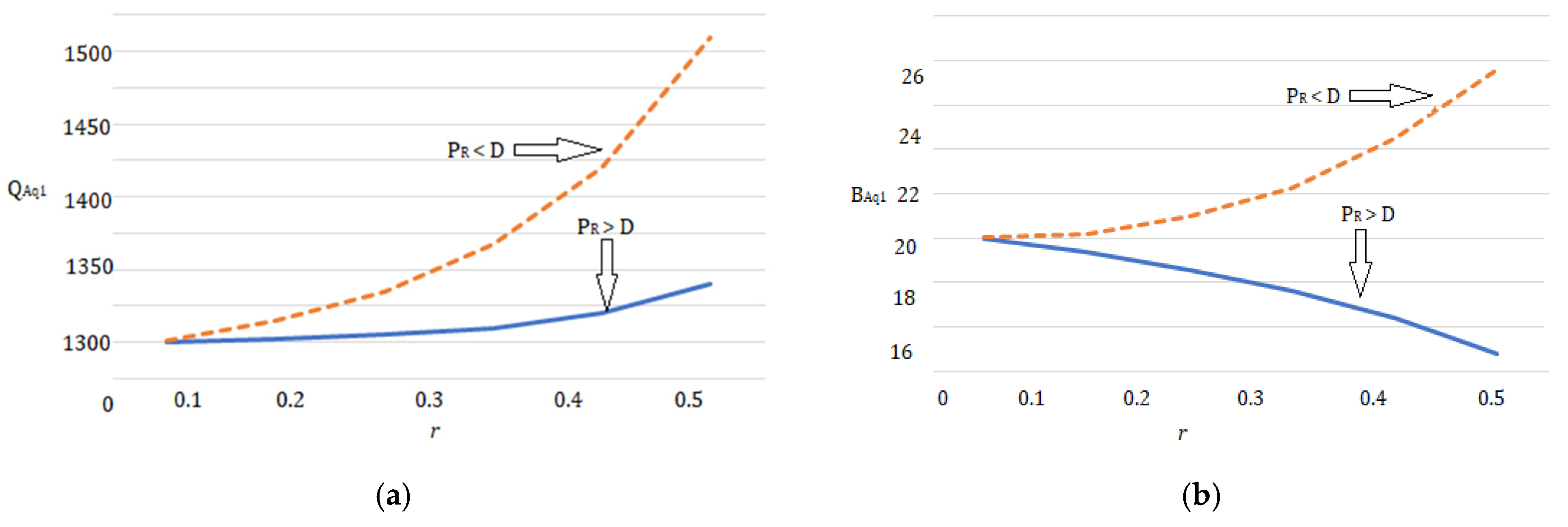
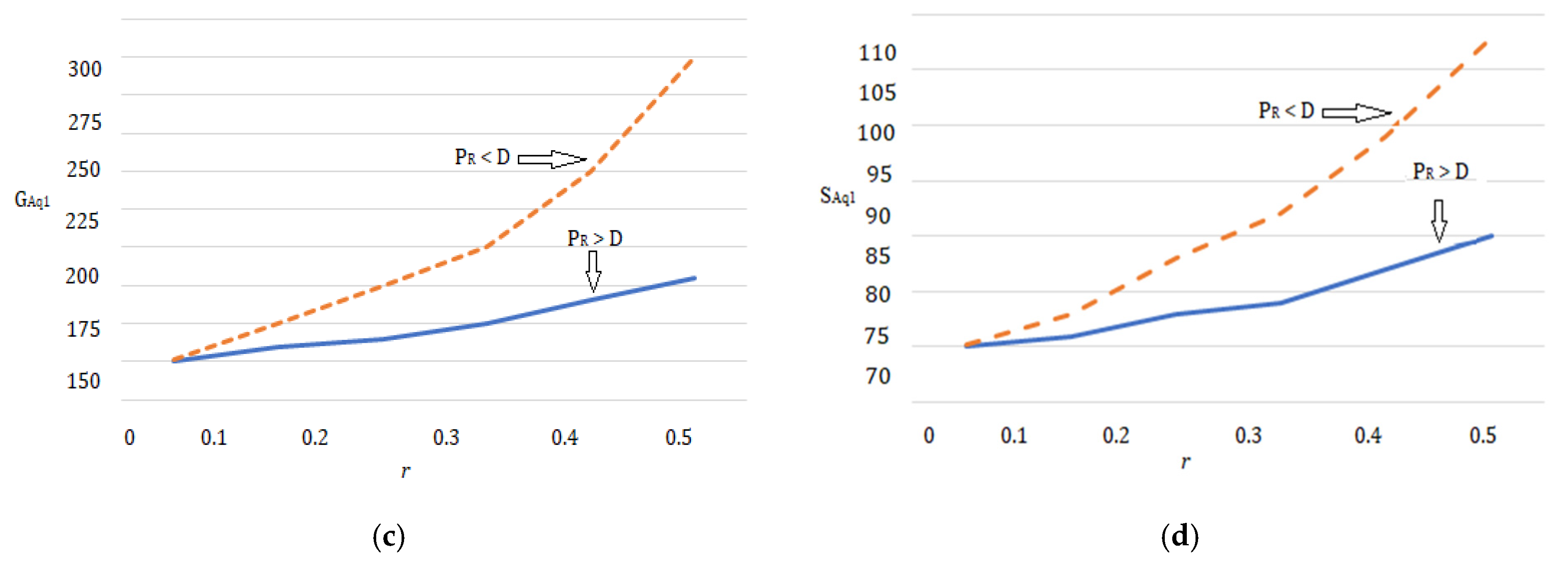
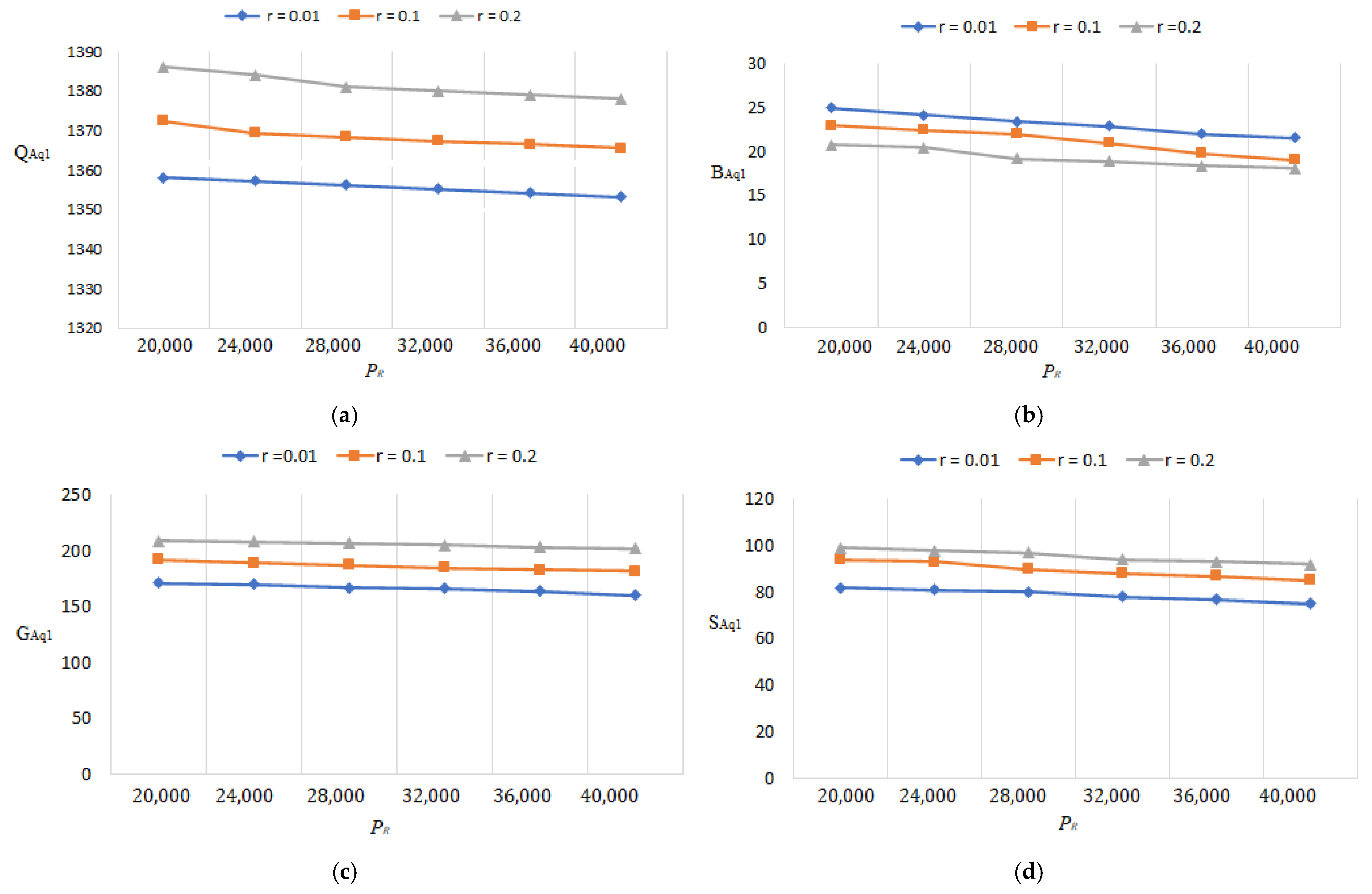
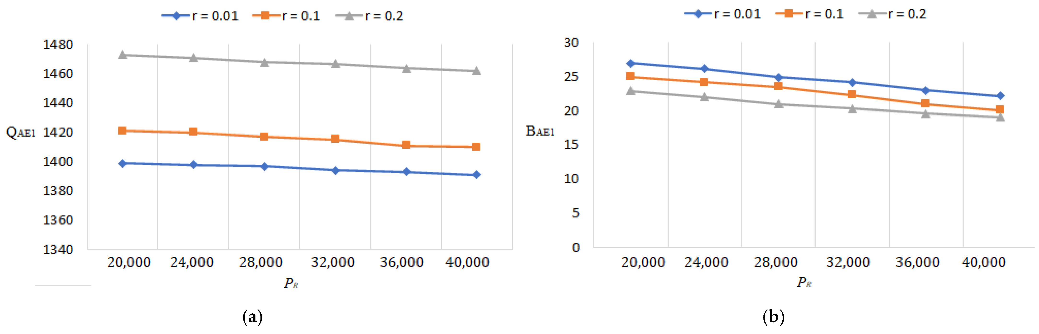
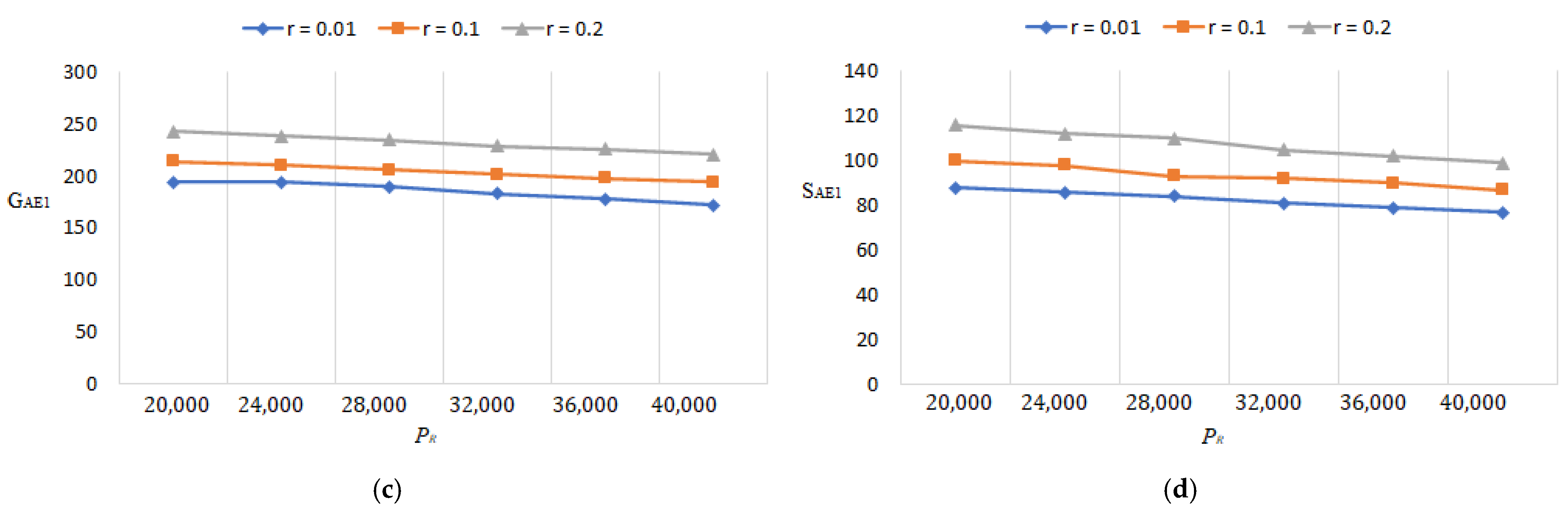
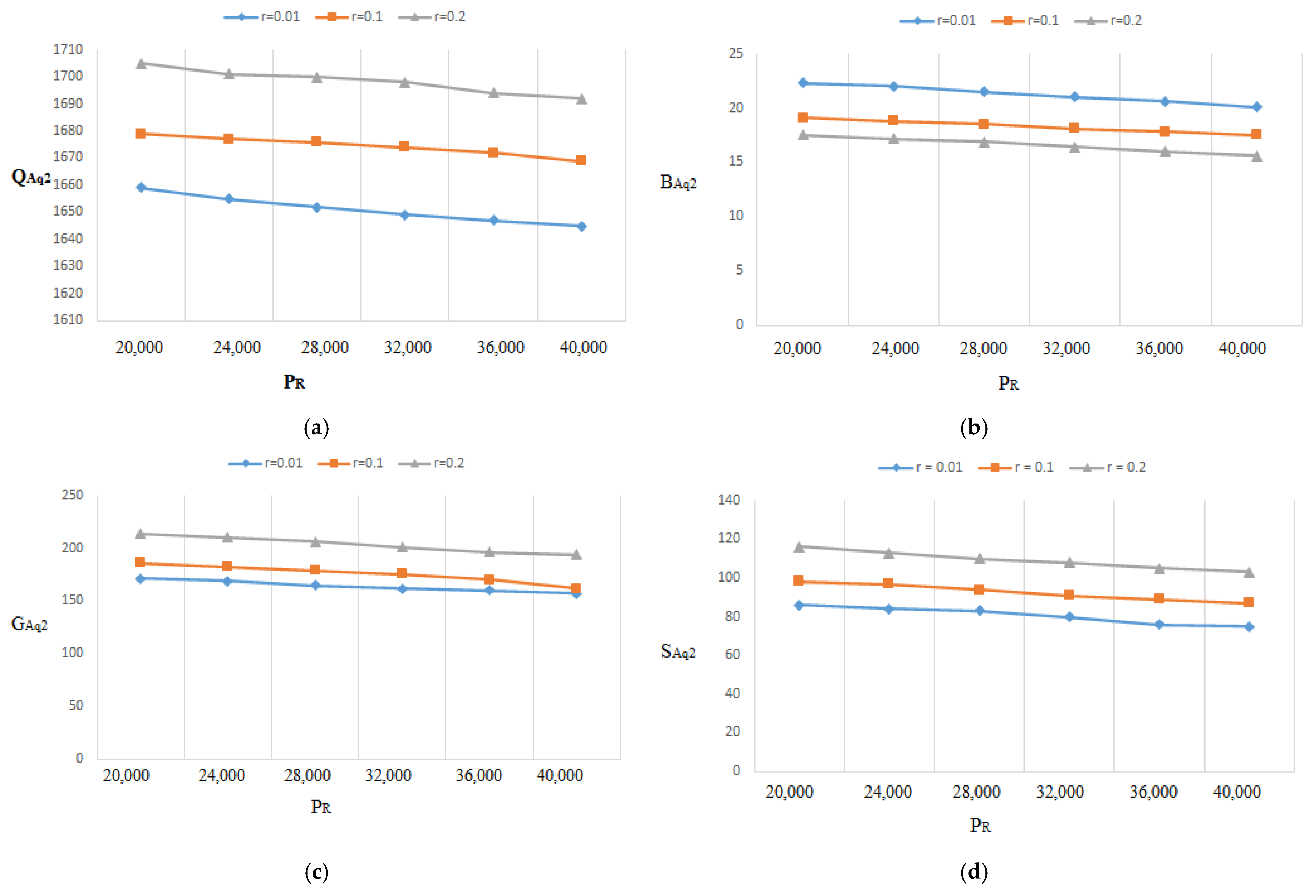
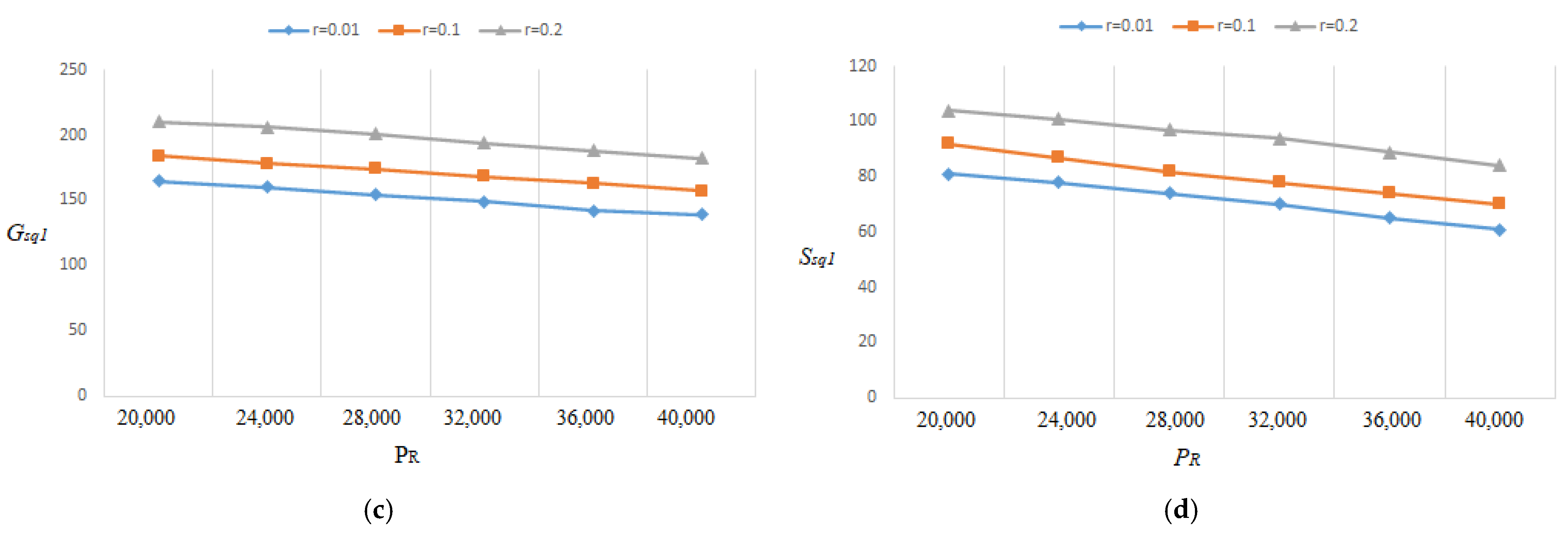
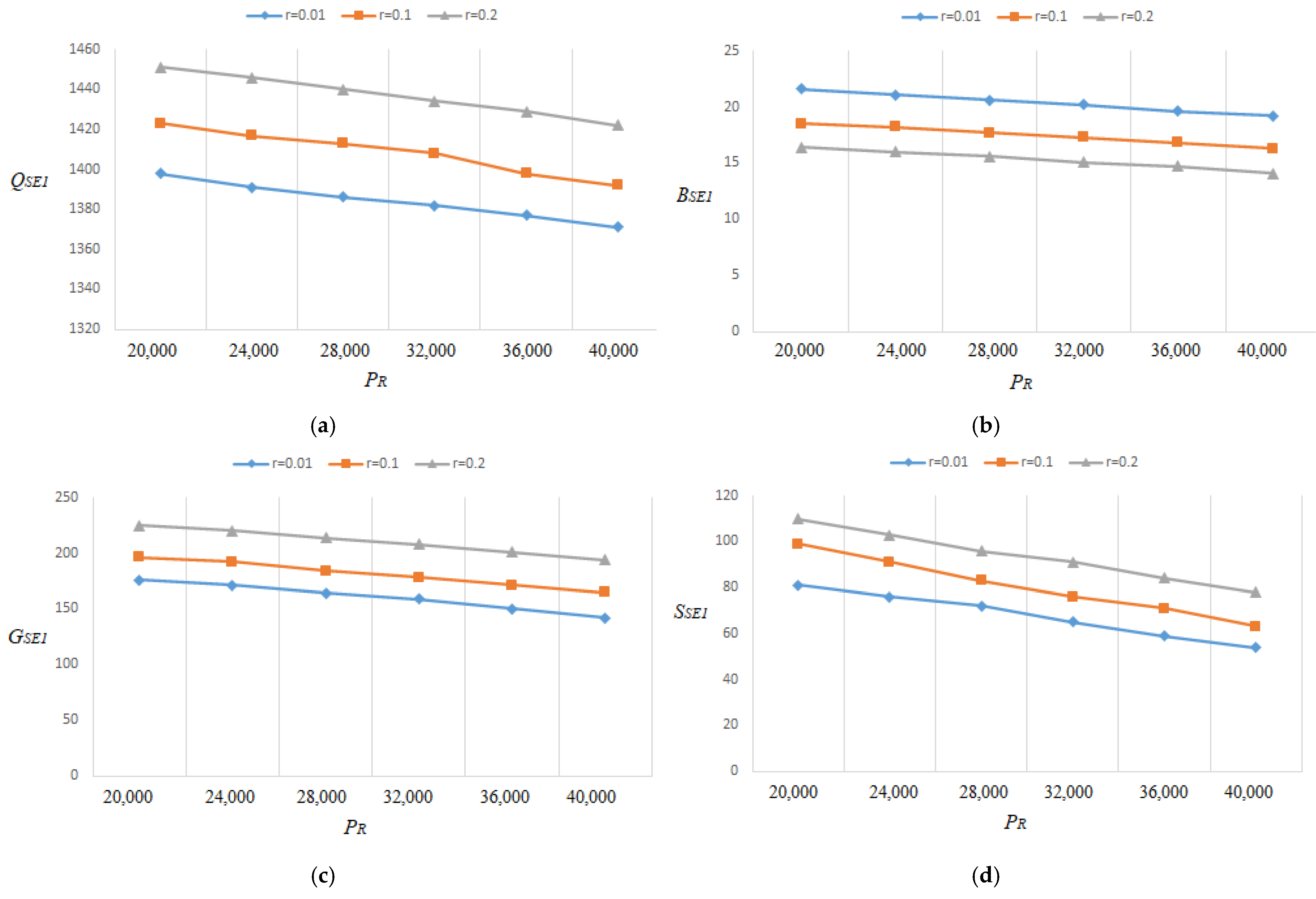
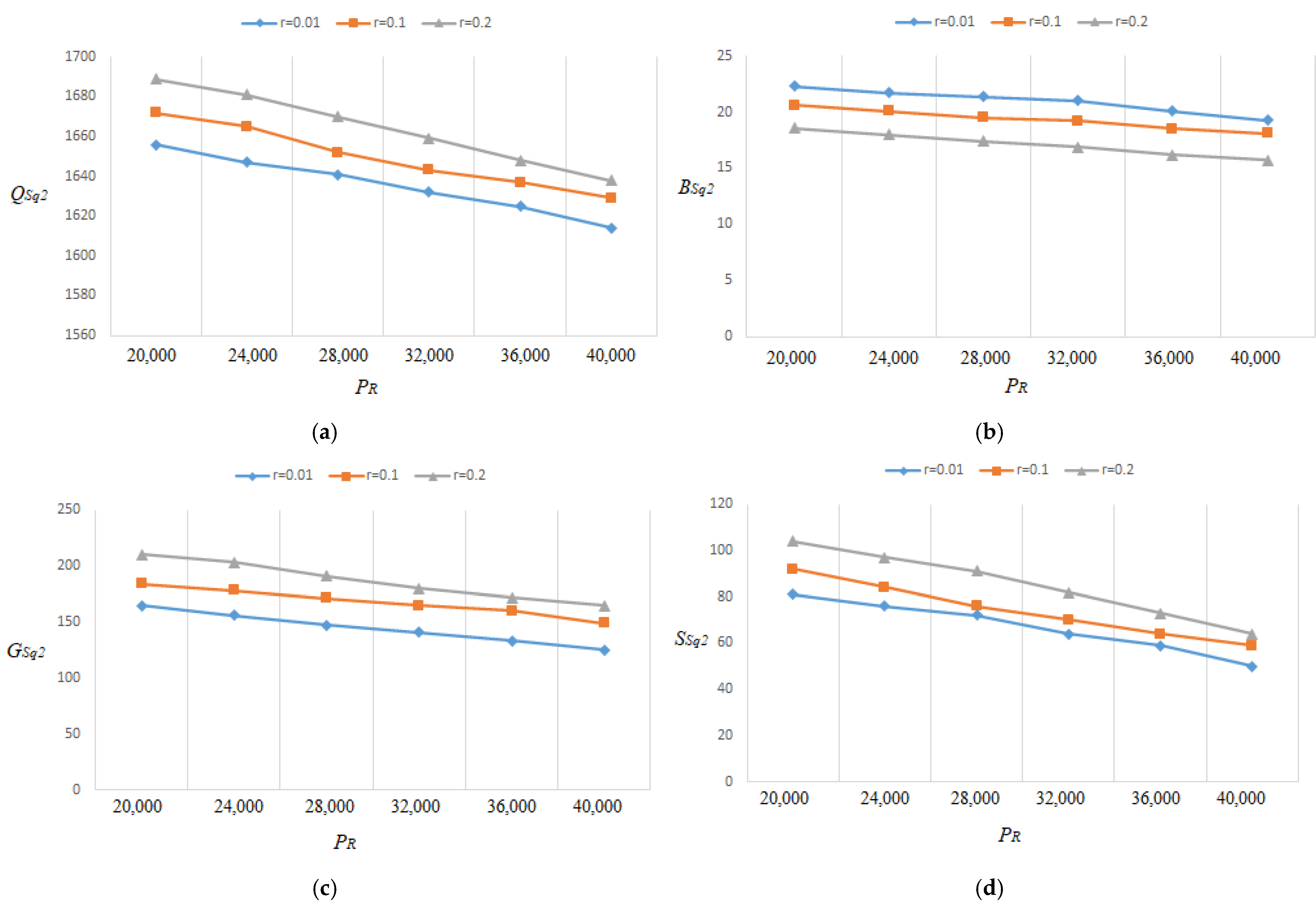
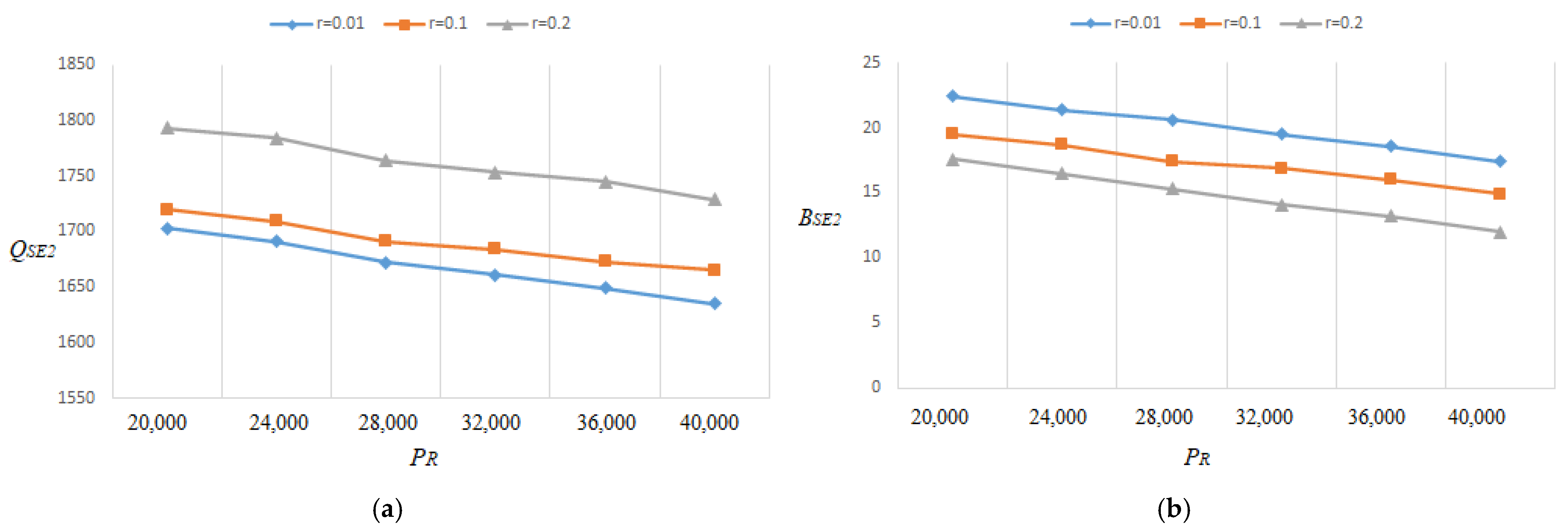
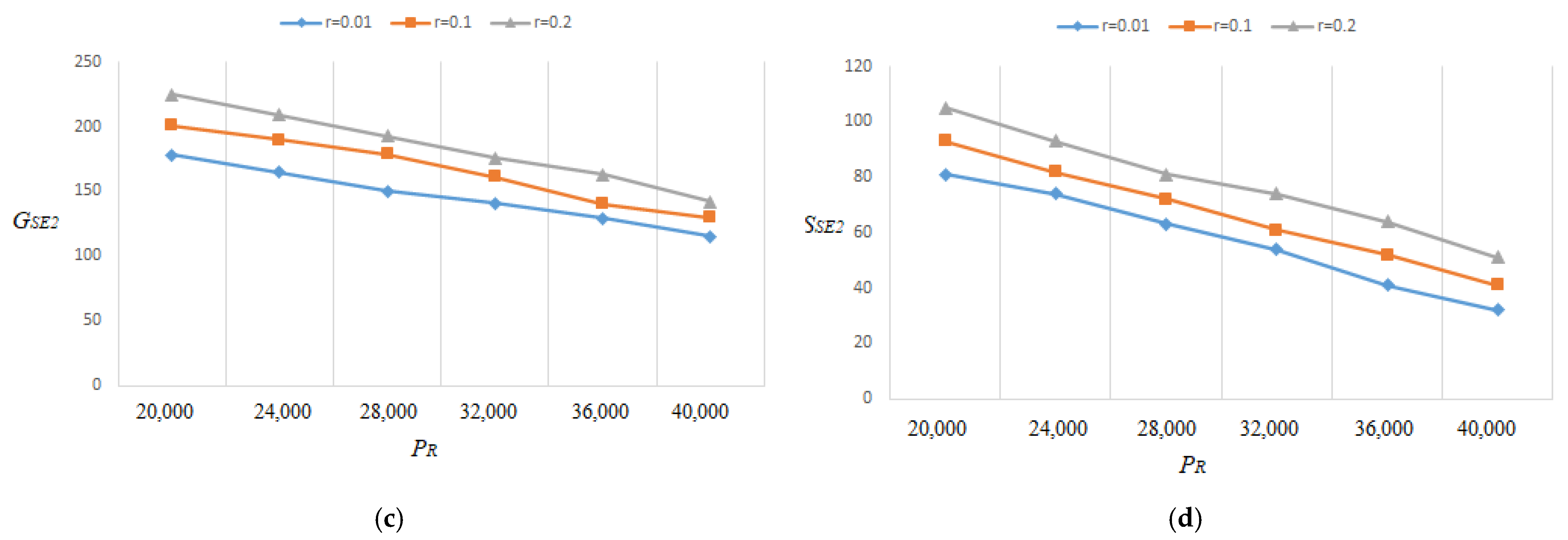
• Since the optimal lot size raises as the percentage of flawed rises, Figure 15a, Figure 16a, Figure 17a, Figure 18a, Figure 19a, Figure 20a, Figure 21a and Figure 22a explore the combined effects of both r and $P_R$ on lot-sizes ($Q_{Aq1},Q_{AE1,}{Q}_{Sq2}, Q_{SE2})$. For large values of r, the optimum lot sizes ($Q_{Aq1},Q_{AE1,}{Q}_{Sq2}, Q_{SE2})$ are more sensitive to changes in the $P_R$ for high values of r than for small values of $r<0.1$, as seen in the picture. As a result, when r > 0.1, it is claimed that lot sizes ($Q_{Aq1},Q_{AE1,}{Q}_{Sq2}, Q_{SE2})$ decreases as $P_R$ increases. Green investments ($G_{Aq1},G_{AE1,}{G}_{Sq2}, G_{SE2})$, on the other hand, are less sensitive to changes in the $P_R$ for large values of r than when the percentage is small ($r<0.1$), as shown in Figure 15c, Figure 16c, Figure 17c, Figure 18c, Figure 19c, Figure 20c, Figure 21c and Figure 22c. Backorder size behavior leads to a similar conclusion. Figure 15b, Figure 16b, Figure 17b, Figure 18b, Figure 19b, Figure 20b, Figure 21b, and Figure 22b indicate that a rise in $P_R$ induces a big fall in ($B_{Aq1},B_{AE1,}{B}_{Sq2}, B_{SE2})$ for values of $r>0.1$.
• Figure 23, Figure 24, Figure 25 and Figure 26 show the CO₂ reduces due to the increase in $C_t$ with r = 0.1.
• The lot-sizes ($Q_{Aq1},Q_{AE1}$) $\mathrm{and}$ green investments ($G_{Aq1},G_{AE1}$) under the asynchronous rework model are slightly lower than the lot sizes ($Q_{Aq2},Q_{AE2}$) $\mathrm{and} \left(G_{Aq2},G_{AE2}\right)$ under the synchronous rework model for the range of r values indicated in Table 2, Table 3, Table 4 and Table 5. When the rework is asynchronous, the backorder is much higher than when it is synchronous for most values of r; though the differences between the backorders are minor, and certain backorders are almost equal for r = 0.4.
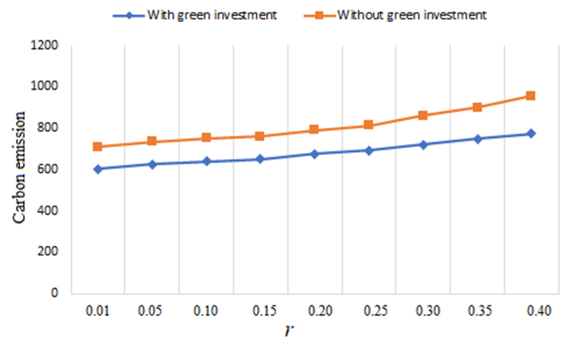
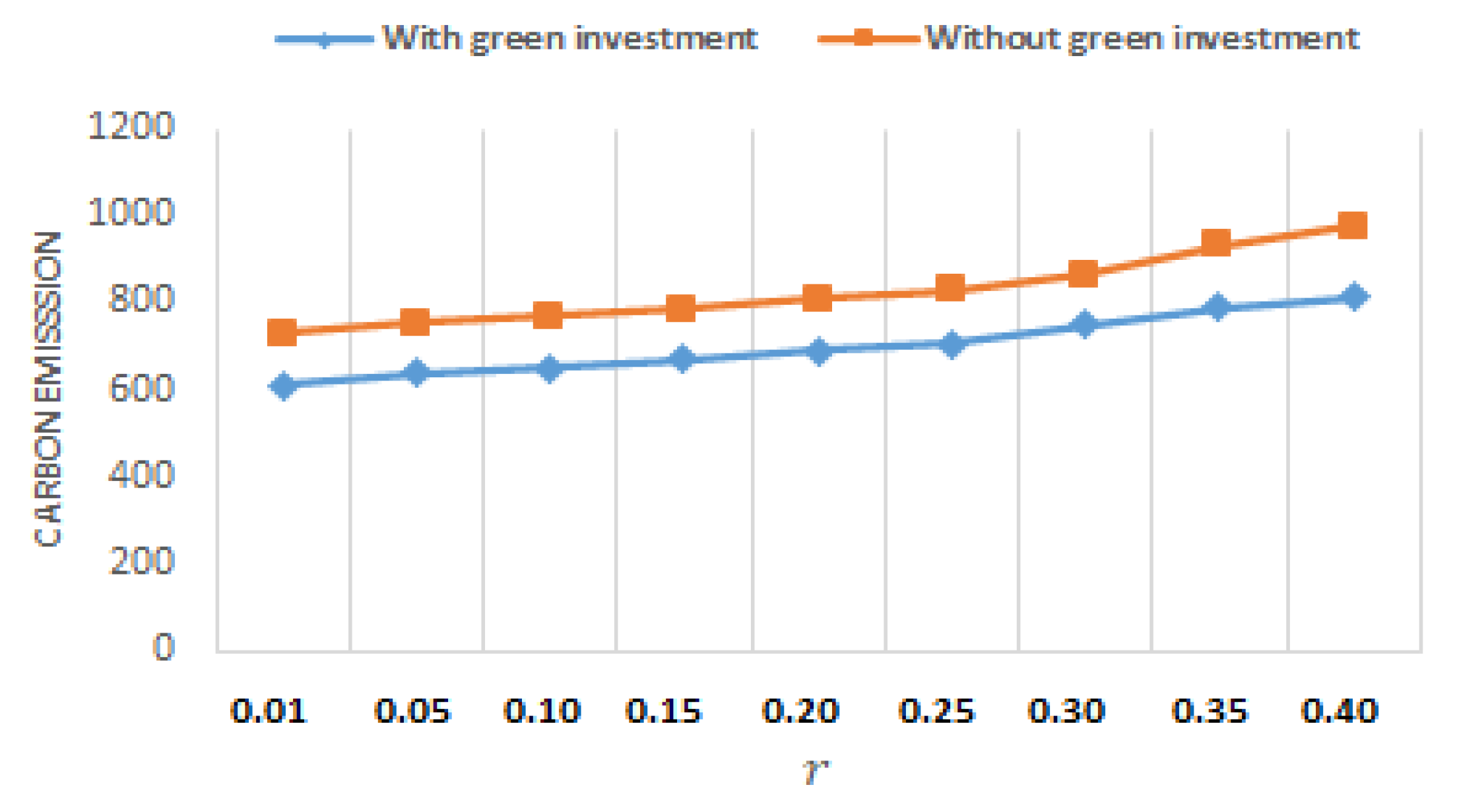
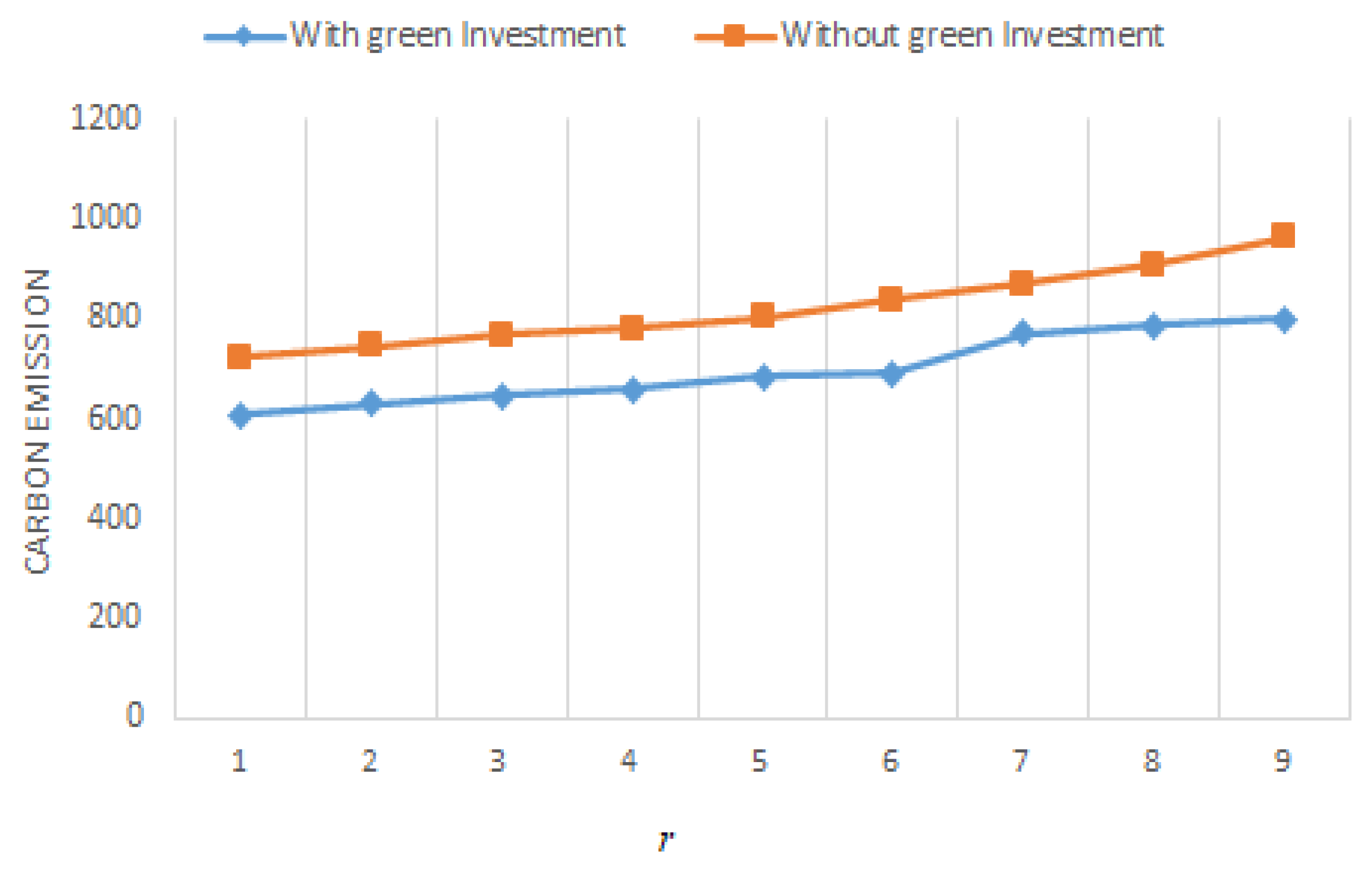
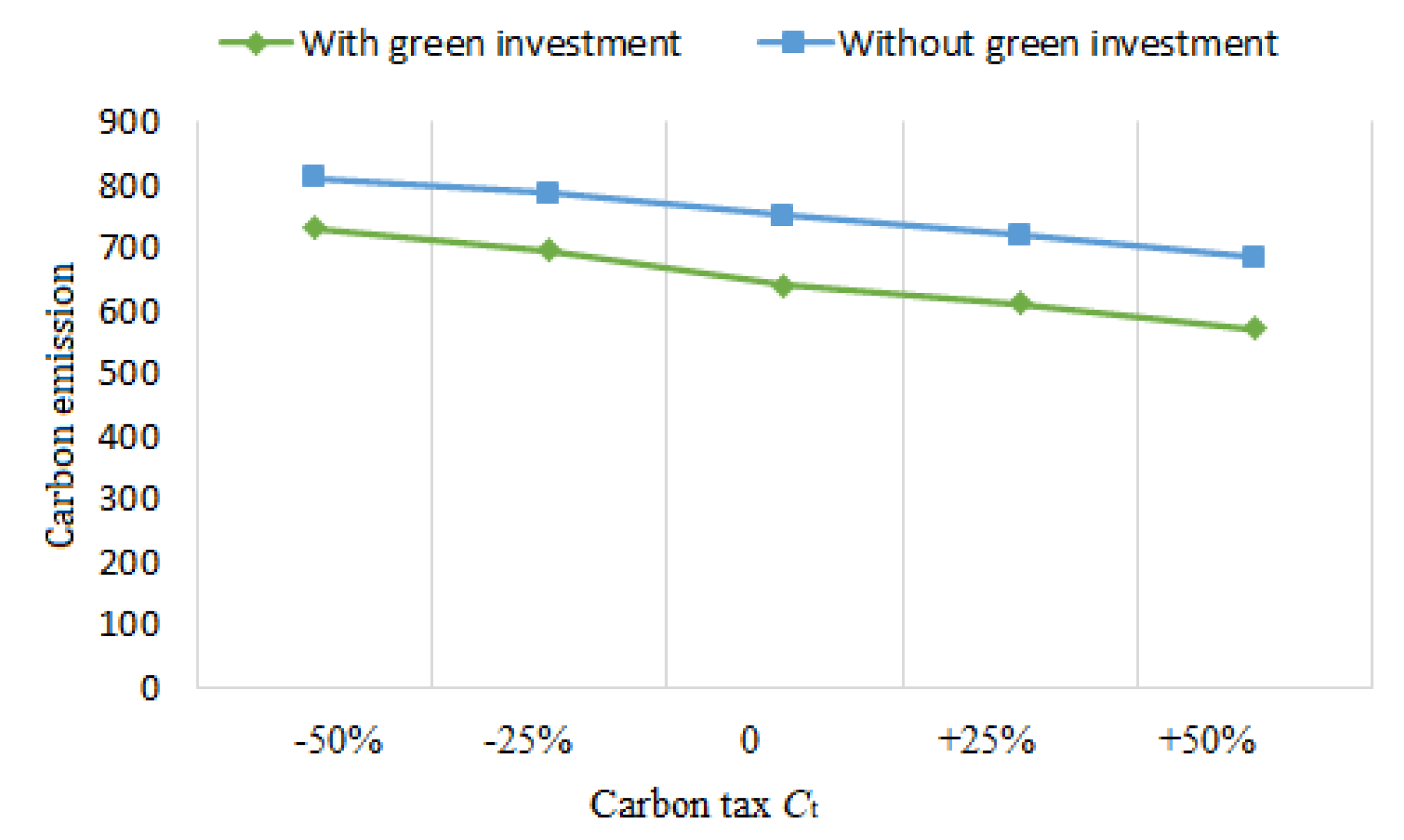
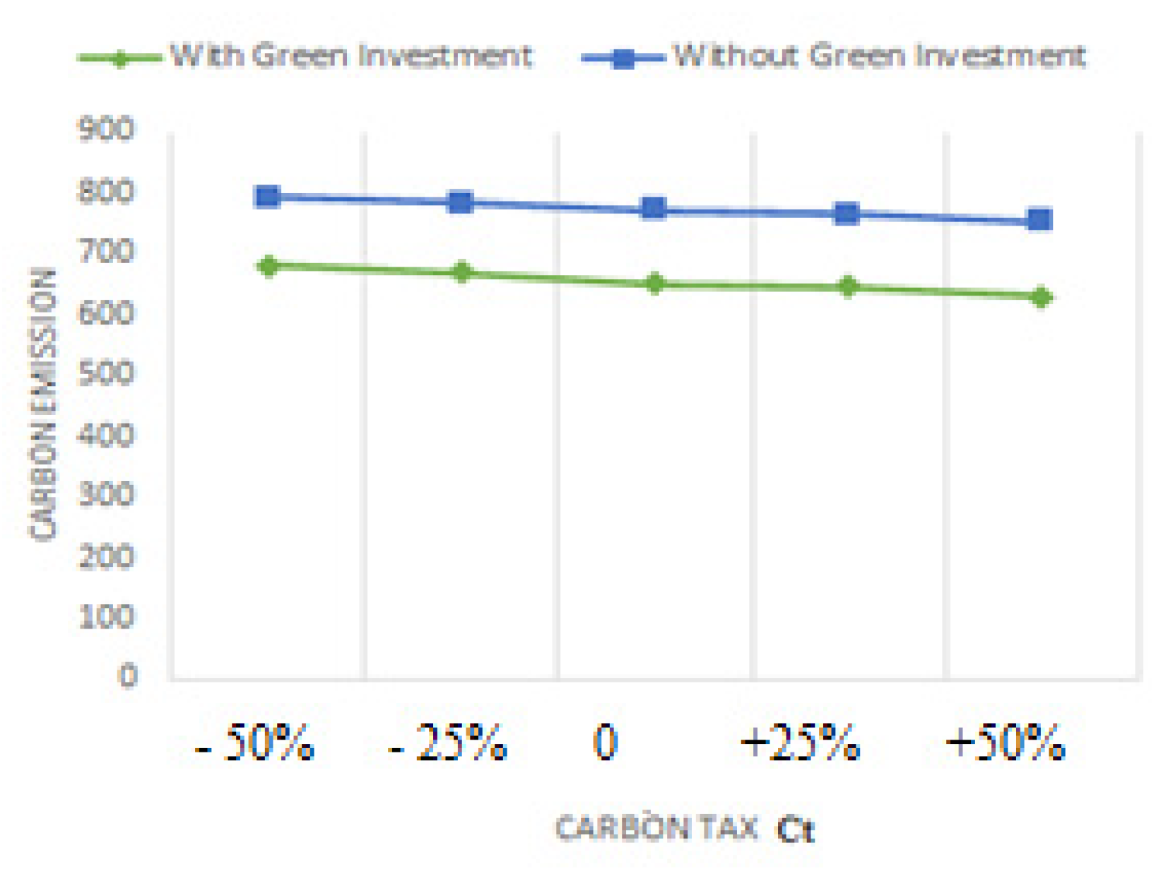
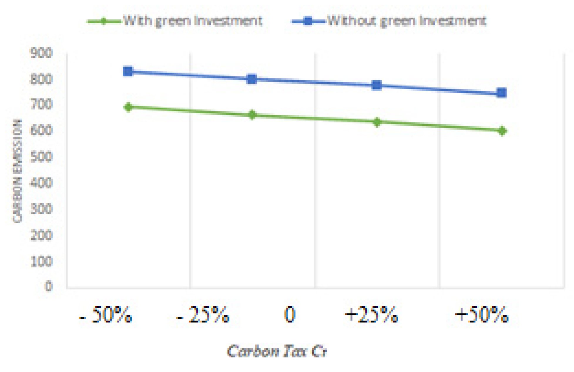
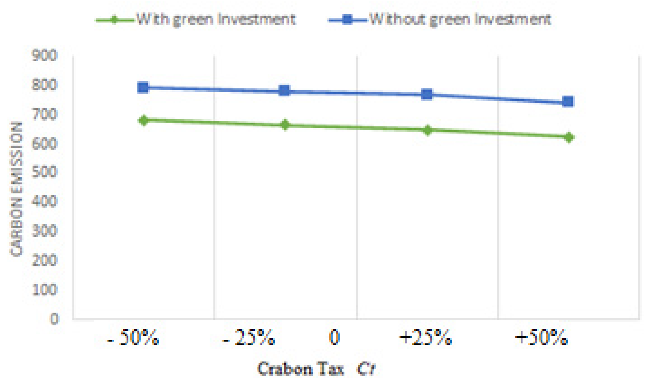
• Our research found that increasing $C_t$ lowers CO₂ levels. The findings of Dwicahyani et al. [40] and Hasanov et al. [41], who found that tariffs had a beneficial effect on CO₂ reduction, are consistent with this conclusion. The firm has new options for lowering CO₂ produced by industrial operations with the use of green technology. The firm will gain from less CO₂ even though green technology has higher direct costs. Studies, including Bai et al. [42] and others, have produced results that are similar.
• According to the findings (Table 2, Table 3, Table 4 and Table 5), the optimal $Q_{Aq1}$,$G_{Aq1}$ and $S_{Aq1}$ grow continuously as r increases, whereas $B_{Aq1}$ progressively decreases as the fraction of defectives rises. The model of Al-Salamah [17] shows a similar pattern, with the exception that the optimal lot size grows faster, and the backorder decreases more slowly than ours. It is worth noting that Al-Salamah’s [17] approach ignores green investment in terms of CO₂ and setup costs. In addition, CO₂ and total cost increase when green technology is not used for both CO₂ and setup costs.
• We may look at Table 4 and Figure 18 and Figure 24 to see how the optimal solutions react when $P_R$ assumptions fluctuate. When r is increased, it is shown that $Q_{Aq2}$ for $P_R<D$ rises more quickly than $Q_{Aq1}$ for $P_R>D$ does if $P_R=2500$ units/year. The optimal backorders respond in a number of ways when r’s value rises. $B_{Aq1}$ declines when r rises, as was previously discovered. On the other hand, raising the value of r causes $B_{Aq2}$ to rise. Additionally, Figure 12 and Figure 24 provide a visual comparison of tax and CO₂ with and without green investment vs. r when $P_R<D$.
• Table 5 and Figure 22 and Figure 26 show how the optimal solutions change when the $P_R$ assumption changes. When $P_R=2500$ units/year, it is seen that, similar to the asynchronous situation when r is increased, $Q_{Aq2}$ for $P_R<D$ raises faster than $Q_{Aq1}$ for $P_R>D$. The optimal backorders react in a number of ways as the value of r increases. As previously discovered, $B_{Aq1}$ lessens as r rises. In contrast, increasing the value of r results in an increase in $B_{Aq2}$. Besides, Figure 12 and Figure 26 depict a visual contrast of CO₂ and taxes with and without green investment vs. r when $P_R<D$.

5.4. Insights and Implications for the Industry

The financial industry has been a significant pillar of human progress since the commencement of the industrial revolution. The global financial sector’s fundamental function is to make optimal use of global savings. Investments that are used wisely can improve people’s quality of life. People have invested their resources in ecologically hazardous initiatives, particularly those that worsen human-induced climate change, as a result of the banking system’s collapse. Despite the fact that finance plays a critical part in the anthropogenic (i.e., human effect on the environment), nothing has been performedto integrate environmental problems into finance. Green investments have obtaineda lot of attention in the financial industry in recent years, which has helped to advance sustainable growth. Green investment is an intersection between environmentally friendly behavior and the financial and business world. On the basis of the results, the managerial insights can be derived as follows:

Making decisions to improve the sustainability of the inventory system, such asoptimizing payout backorder and lot size, may assist the green inventory model. Businesses will be better able to concentrate on reducing the overall inventory in storage facilities if CO₂ costs are included in the model. This will help to reduce the price of CO₂ from storage. Firms must focus on transportation if they want to reduce overall costs.

This paper demonstrates that shifting to sustainable invention significantly affects the inventory system. Producers can use green technology to reduce CO₂ from manufacturing, transport, and storage to abide by CO₂ price rules. Green technology includes recycling technology, eco-friendly polymers, green chemical processes, and renewable energy (solar, wind, hydro). Policymakers must thus sensibly prefer the optimal kind of green technology. They must take into account additional factors in addition to economic aspects when choosing the exact technology, such as the technology’s ability to reduce pollution and compatibility with machines.

Managers can adjust the production rate using the suggested approach by controlling production allocation. A strategy of production rate adjustment is essential when the rate of production has a substantial impact on the volume of CO₂ generated. According to our research, the system can profit from a decrease in production rate by balancing supply and demand and reducing CO₂. Unfortunately, this benefit was not accessible since earlier inventory models did not take these limitations into account. Our research shows that the decision-making criteria and ultimate cost are affected by concerns about CO₂. The study’s conclusions also provide a roadmap that inventory decision-makers may use to achieve successful long-term inventory management.

6. Conclusions

Today an increasing number of businesses have made sustainability a top priority in their strategy and operations to boost growth and global competitiveness. This movement currently encompasses several well-known businesses from a wide range of industries, considerably beyond the small number of firms thatpreviously positioned themselves as green. This study offers an extension to anearlier study that intends at cutting the CO₂ and setup cost simultaneously in a backorder situation. This research considers an imperfect production process where a fraction of the items is faulty, and the firm employs a rework approach to rectify the faulty items under two realistic scenarios: asynchronous and synchronous. We used twoforms of green investment to attain the lowest cost in terms of optimal lot size, backorder and decreased setup cost while reducing CO₂. We have formulated eight mathematical models under various problem settings.Iterativesolution approaches are derived and proved analytically and numerically for all models. The examples show how the lot size grows and the backorder reduces as the fraction of defects for asynchronous rework with a rework rate greater than the demand rises.

The proposed model can be expanded upon in future research because this study has some limitations. The failure of this research to demonstrate the impact of COVID-19 on the company’s transportation system is a limitation. The pandemic may, therefore, affect customer demand, leading to a fluctuating demand that changes over time. This type of work could be a great extension of this study. We also missedincluding the effect of learning onquality. If so, a more intriguing extension would be to look into whether investing in screening-related learning is worthwhile. Moreover, the limitations of utilizing a CO₂ reduction process, such as Green Lean Six Sigma, cap-and-trade and carbon offsets, were lacking inthis research.

References

1. Rosenblatt, M.J.; Lee, H.L. Economic Production Cycles with Imperfect Production Processes. IIE Trans. 1986, 18, 48–55. [Google Scholar] [CrossRef]
2. Khouja, M.; Abraham, M. An economic production lot size model with imperfect quality and variable production rate. J. Oper. Res. Soc. 1994, 45, 1405–1417. [Google Scholar] [CrossRef]
3. Brojeswar, P.; Shib, S.S.; Kripasindhu, C. A mathematical model on EPQ for stochastic demand in an imperfect production system. J. Manuf. Syst. 2013, 32, 260–270. [Google Scholar]
4. Hsu, J.-T.; Hsu, L.-F. Two EPQ models with imperfect production processes, inspection errors, planned backorders, and sales returns. Comput. Industr. Eng. 2013, 64, 389–402. [Google Scholar] [CrossRef]
5. Taleizadeh, A.A.; Cárdenas-Barrón, L.E.; Mohammadi, B. A deterministic multi product single machine EPQ model with backordering, scraped products, rework and interruption in manufacturing process. Int. J. Prod. Econ. 2014, 150, 9–27. [Google Scholar] [CrossRef]
6. Hsu, L.-F.; Hsu, J.-T. Economic production quantity (EPQ) models under an imperfect production process with shortages backordered. Int. J. Syst. Sci. 2014, 47, 852–867. [Google Scholar] [CrossRef]
7. Ganesan, S.; Uthayakumar, R. EPQ models for an imperfect manufacturing system considering warm-up production run, shortages during hybrid maintenance period and partial backordering. Adv. Ind. Manuf. Eng. 2020, 1, 100005. [Google Scholar] [CrossRef]
8. De Sujit, K.; Nayak, P.K.; Khan, A.; Bhattacharya, K.; Smarandache, F. Solution of an EPQ model for imperfect production process under game and neutrosophic fuzzy approach. Appl. Soft Comput. 2020, 93, 106397. [Google Scholar]
9. Dipankar, B.; Apratim, G. Economic production lot sizing under imperfect quality, on-line inspection, and inspection errors: Full vs. sampling inspection. Comput. Industr. Eng. 2021, 160, 107565. [Google Scholar]
10. Liu, J.J.; Yang, P. Optimal lot-sizing in an imperfect production system with homogeneous reworkable jobs. Eur. J. Oper. Res. 1996, 91, 517–527. [Google Scholar] [CrossRef]
11. Hayek, P.A.; Salameh, M.K. Production lot sizing with the reworking of imperfect quality items produced. Prod. Plan. Control 2001, 12, 584–590. [Google Scholar] [CrossRef]
12. Liao, G.-L.; Chen, Y.H.; Sheu, S.-H. Optimal economic production quantity policy for imperfect process with imperfect repair and maintenance. Eur. J. Oper. Res. 2009, 195, 348–357. [Google Scholar] [CrossRef]
13. Liao, G.-L.; Sheu, S.-H. Economic production quantity model for randomly failing production process with minimal repair and imperfect maintenance. Int. J. Prod. Econ. 2011, 130, 118–124. [Google Scholar] [CrossRef]
14. Krishnamoorthi, C.; Panayappan, S. An EPQ Model with Imperfect Production Systems with Rework of Regular Production and Sales Return. Am. J. Oper. Res. 2012, 2, 225–234. [Google Scholar] [CrossRef] [Green Version]
15. Shah, N.H.; Patel, D.G.; Shah, D.B. EPQ model for returned/reworked inventories during imperfect production process under price-sensitive stock-dependent demand. Oper. Res. 2018, 18, 343–359. [Google Scholar] [CrossRef]
16. Nihar, S.; Marianthi, I.; John, W. Synchronous and asynchronous decision-making strategies in supply chains. Comput. Chem. Eng. 2013, 71, 116–129. [Google Scholar]
17. Al-Salamah, M. Economic production quantity in an imperfect manufacturing process with synchronous and asynchronous flexible rework rates. Oper. Res. Perspect. 2019, 6, 100103. [Google Scholar] [CrossRef]
18. Coates, E.R.; Sarker, B.R.; Ray, T.G. Manufacturing setup cost reduction. Comput. Industr. Eng. 1996, 31, 111–114. [Google Scholar] [CrossRef]
19. Sarkar, B.; Moon, I. Improved quality, setup cost reduction, and variable backorder costs in an imperfect production process. Int. J. Prod. Econ. 2014, 155, 204–213. [Google Scholar] [CrossRef]
20. Porteus, E.L. Optimal Lot Sizing, Process Quality Improvement and Setup Cost Reduction. Oper. Res. 1986, 34, 137–144. [Google Scholar] [CrossRef]
21. Hou, K.-L. An EPQ model with setup cost and process quality as functions of capital expenditure. Appl. Math. Model. 2007, 31, 10–17. [Google Scholar] [CrossRef]
22. Freimer, M.; Thomas, D.; Tyworth, J. The value of setup cost reduction and process improvement for the economic production quantity model with defects. Eur. J. Oper. Res. 2006, 173, 241–251. [Google Scholar] [CrossRef]
23. Nye, T.J.; Jewkes, E.M.; Dilts, D.M. Optimal investment in setup reduction in manufacturing systems with WIP inventories. Eur. J. Oper. Res. 2002, 135, 128–141. [Google Scholar] [CrossRef]
24. Sarkar, B.; Chaudhuri, K.; Moon, I. Manufacturing setup cost reduction and quality improvement for the distribution free continuous-review inventory model with a service level constraint. J. Manuf. Syst. 2015, 34, 74–82. [Google Scholar] [CrossRef]
25. Tiwari, S.; Kazemi, N.; Modak, N.M.; Cárdenas-Barrón, L.E.; Sarkar, S. The effect of human errors on an integrated stochastic supply chain model with setup cost reduction and backorder price discount. Int. J. Prod. Econ. 2020, 226, 107643. [Google Scholar] [CrossRef]
26. Bouchery, Y.; Ghaffari, A.; Jemai, Z.; Dallery, Y. Including sustainability criteria into inventory models. Eur. J. Oper. Res. 2012, 222, 229–240. [Google Scholar] [CrossRef] [Green Version]
27. Benjaafar, S.; Li, Y.; Daskin, M. Carbon Footprint and the Management of Supply Chains: Insights From Simple Models. IEEE Trans. Autom. Sci. Eng. 2013, 10, 99–116. [Google Scholar] [CrossRef]
28. Toptal, A.; Özlü, H.; Konur, D. Joint decisions on inventory replenishment and emission reduction investment under different emission regulations. Int. J. Prod. Res. 2014, 52, 243–269. [Google Scholar] [CrossRef] [Green Version]
29. Dye, C.-Y.; Yang, C.-T. Sustainable trade credit and replenishment decisions with credit-linked demand under carbon emission constraints. Eur. J. Oper. Res. 2015, 244, 187–200. [Google Scholar] [CrossRef]
30. Qin, J.; Bai, X.; Xia, L. Sustainable Trade Credit and Replenishment Policies under the Cap-And-Trade and Carbon Tax Regulations. Sustainability 2015, 7, 16340–16361. [Google Scholar] [CrossRef] [Green Version]
31. Datta, T.K. Effect of Green Technology Investment on a Production-Inventory System with Carbon Tax. Adv. Oper. Res. 2017, 2017, 4834839. [Google Scholar] [CrossRef] [Green Version]
32. Huang, Y.-S.; Fang, C.-C.; Lin, Y.-A. Inventory management in supply chains with consideration of Logistics, green investment and different carbon emissions policies. Comput. Ind. Eng. 2019, 139, 106207. [Google Scholar] [CrossRef]
33. Mishra, U.; Wu, J.-Z.; Sarkar, B. A sustainable production-inventory model for a controllable carbon emissions rate under shortages. J. Clean. Prod. 2020, 256, 120268. [Google Scholar] [CrossRef]
34. Hasan, R.; Roy, T.C.; Daryanto, Y.; Wee, H.-M. Optimizing inventory level and technology investment under a carbon tax, cap-and-trade and strict carbon limit regulations. Sustain. Prod. Consum. 2020, 25, 604–621. [Google Scholar] [CrossRef]
35. Kaswan, M.S.; Rathi, R.; Reyes, J.A.G.; Antony, J. Exploration and Investigation of Green Lean Six Sigma Adoption Barriers for Manufacturing Sustainability. IEEE Trans. Eng. Manag. 2021, 1–15. [Google Scholar] [CrossRef]
36. Kaswan, M.S.; Rathi, R.; Garza-Reyes, J.A.; Antony, J. Green lean six sigma sustainability–oriented project selection and implementation framework for manufacturing industry. Int. J. Lean Six Sigma 2022. [Google Scholar] [CrossRef]
37. Rathi, R.; Kaswan, M.S.; Garza-Reyes, J.A.; Antony, J.; Cross, J. Green Lean Six Sigma for improving manufacturing sustainability: Framework development and validation. J. Clean. Prod. 2022, 345, 131130. [Google Scholar] [CrossRef]
38. Mohan, J.; Rathi, R.; Kaswan, M.S.; Nain, S.S. Green lean six sigma journey: Conceptualization and realization. Mater. Today Proc. 2021, 50, 1991–1998. [Google Scholar] [CrossRef]
39. Ouyang, L.-Y.; Chen, C.-K.; Chang, H.-C. Quality improvement, setup cost and lead-time reductions in lot size reorder point models with an imperfect production process. Comput. Oper. Res. 2002, 29, 1701–1717. [Google Scholar] [CrossRef]
40. Dwicahyani, A.R.; Jauhari, W.A.; Rosyidi, C.N.; Laksono, P.W. Inventory decisions in a two-echelon system with remanufacturing, carbon emission and energy effects. Cogent Eng. 2017, 4, 1–17. [Google Scholar] [CrossRef]
41. Hasanov, P.; Jaber, M.; Tahirov, N. Four-level closed loop supply chain with remanufacturing. Appl. Math. Model. 2019, 66, 141–155. [Google Scholar] [CrossRef]
42. Bai, Q.; Xua, J.; Chauhan, S.C. Effects of sustainability investment and risk aversion on a two-stage supply chain coordination under a carbon tax policy. Comp. Industr. Eng. 2020, 142, 106324. [Google Scholar] [CrossRef]
Figure 1. Sector global greenhouse gas CO2.
Sustainability 14 16999 g001
Figure 2. Schematic diagram of the research methodology.
Sustainability 14 16999 g002
Figure 3. Inventory curves of perfect items when P R > D (asynchronous rework). Bule represents available stock, and purple represents out of stock.
Sustainability 14 16999 g003
Figure 4. Inventory curves of the flawed items when P R > D (asynchronous rework).
Sustainability 14 16999 g004
Figure 5. Inventory curves of perfect items with asynchronous rework and P R < D . Grey represents available stock, and purple represents out of stock.
Sustainability 14 16999 g005
Figure 6. Inventory curves of perfect items with synchronous rework. Blue represents available stock, and purple represents out of stock.
Sustainability 14 16999 g006
Figure 7. Inventory curves of flawed items with synchronous rework.
Sustainability 14 16999 g007
Figure 8. Inventory curves of perfect products with synchronous rework when P R < D . Blue represents available stock, and purple represents out of stock.
Sustainability 14 16999 g008
Figure 9. Comparison of the CO2 when P R > D with and without green investment vs. r.
Sustainability 14 16999 g009
Figure 10. Comparison of the CO2 when P R < D with and without green investment vs. r.
Sustainability 14 16999 g010
Figure 11. Comparison of CO2 with and without green investment vs. r when P R > D .
Sustainability 14 16999 g011
Figure 12. CO2 comparison with and without green investment vs. r.
Sustainability 14 16999 g012
Figure 13. Optimal Q A q 1 ,   B A q 1 ,   G A q 1 , S A q 1 vs. r under the asynchronous rework (Quadratic case). (a) Q A q 1 vs. r; (b) B A q 1 vs. r; (c) G A q 1 vs. r; (d) S A q 1 vs. r.
Sustainability 14 16999 g013aSustainability 14 16999 g013b
Figure 14. Optimal Q A E 1 ,   B A E 1 ,   G A E 1 , S A E 1 vs. r under the asynchronous rework (Exponential case). (a) Q A E 1 vs. r; (b) B A E 1 vs. r; (c) G A E 1 vs. r; (d) S A E 1 vs. r.
Sustainability 14 16999 g014
Figure 15. How the Q A q 1 ,   B A q 1 ,   G A q 1 , S A q 1 changes with the rate of asynchronous rework P R > D (Quadratic case). (a) Quantity lot size Q A q 1 variations with P R ; (b) Backorder B A q 1 variations with P R ; (c) Green investment G A q 1 variations with P R ; (d) Setup cost S A q 1 variations with P R .
Sustainability 14 16999 g015
Figure 16. How the Q A E 1 ,   B A E 1 ,   G A E 1 , S A E 1 changes with the rate of asynchronous rework P R > D (Exponential case). (a) Quantity lot size Q A E 1 variations P R ; (b) Backorder B A E 1 variations with P R ; (c) Green investment G A E 1 variations with P R ; (d) Setup cost S A E 1 variations with P R .
Sustainability 14 16999 g016aSustainability 14 16999 g016b
Figure 17. How the Q A q 2 ,   B A q 2 ,   G A q 2 , S A q 2 changes with the rate of asynchronous rework P R < D (Quadratic case). (a) Quantity lot size Q A q 2 variations with P R ; (b) Backorder B A q 2 variations with P R ; (c) Green investment G A q 2 variations with P R ; (d) Setup cost S A q 2 variations with P R .
Sustainability 14 16999 g017
Figure 18. How the Q A E 2 ,   B A E 2 ,   G A E 2 , S A E 2 changes with the rate of asynchronous rework P R < D (Exponential case). (a) Quantity lot size Q A E 2 variations with P R ; (b) Backorder B A E 2 variations with P R ; (c) Green investment G A E 2 variations with P R ; (d) Setup cost S A E 2 variations with P R .
Sustainability 14 16999 g018
Figure 19. How the Q S q 1 ,   B S q 1 ,   G S q 1 , S S q 1 changes with the rate of synchronous rework P R (Quadratic case). (a) Quantity lot size Q S q 1 variations with P R ; (b) Backorder B S q 1 variations with P R ; (c) Green investment G S q 1 variations with P R ; (d) Setup cost S S q 1 variations with P R .
Sustainability 14 16999 g019aSustainability 14 16999 g019b
Figure 20. How the Q S E 1 ,   B S E 1 ,   G S E 1 , S S E 1 changes with the rate of synchronous rework P R (Exponential case). (a) Quantity lot size Q S E 1 variations with P R ; (b) Backorder B S E 1 variations with P R ; (c) Green investment G S E 1 variations with P R ; (d) Setup cost S S E 1 variations with P R .
Sustainability 14 16999 g020
Figure 21. How the Q S q 2 ,   B S q 2 ,   G S q 2 , S S q 2 changes with the rate of synchronous rework P R (Quadratic case). (a) Quantity lot size Q S q 2 variations with P R ; (b) Backorder B S q 2 variations with P R ; (c) Green investment G S q 2 variations with P R ; (d) Setup cost S S q 2 variations with P R .
Sustainability 14 16999 g021
Figure 22. How the Q S E 2 ,   B S E 2 ,   G S E 2 , S S E 2 changes with the rate of synchronous rework P R (Exponential case). (a) Quantity lot size Q S E 2 variations with P R ; (b) Backorder B S E 2 variations with P R ; (c) Green investment G S E 2 variations with P R ; (d) Setup cost S S E 2 variations with P R .
Sustainability 14 16999 g022aSustainability 14 16999 g022b
Figure 23. CO2 for various C t with r = 0.1 when P R > D .
Sustainability 14 16999 g023
Figure 24. CO2 for various C t with r = 0.1 when P R < D .
Sustainability 14 16999 g024
Figure 25. CO2 for various C t with r = 0.1 when P R > D .
Sustainability 14 16999 g025
Figure 26. CO2 for various C t with r = 0.1.
Sustainability 14 16999 g026